| Issue |
A&A
Volume 522, November 2010
|
|
|---|---|---|
| Article Number | A11 | |
| Number of page(s) | 13 | |
| Section | Extragalactic astronomy | |
| DOI | https://doi.org/10.1051/0004-6361/201014179 | |
| Published online | 27 October 2010 | |
Optically faint X-ray sources in the Chandra deep field North: Spitzer constraints
1
Max-Planck-Institut für Extraterrestrische Physik
Giessenbachstraße
85748
Garching
Germany
e-mail: This email address is being protected from spambots. You need JavaScript enabled to view it.
2
Osservatorio Astronomico di Bologna/INAF,
via Ranzani 1, 40127
Bologna,
Italy
3
Institute of Astronomy and Astrophysics, National Observatory of
Athens, I. Metaxa & V.
Pavlou str., Palaia Penteli, 15236
Athens,
Greece
4
Max-Planck-Institut für Plasmaphysik, Boltzmannstraße 2, 85748
Garching,
Germany
5
Technische Universität München, Fakultät für Physik, James-Frank-Straße,
85748
Garching,
Germany
Received:
1
February
2010
Accepted:
2
June
2010
Abstract
We investigate the properties of the most optically faint sources in the GOODS-N area (RAB > 26.5). These extremely optically faint populations present an uncharted territory although they represent an appreciable fraction of the X-ray sources in the GOODS-N field. The optically faint sources are believed to contain either red active galactic nuclei (AGN) at moderate redshifts or possibly quasi stellar objects (QSOs) at very high redshift. We compile our sample by first finding the 3.6 μm IRAC counterparts of the X-ray sources and in turn by searching for the optical counterparts of the IRAC sources. No counterparts were found for 35 objects in the R-band Subaru optical images. Of these, 18 have HST ACS counterparts, while the remaining have no optical counterparts. The vast majority of our 35 sources are classified as extremely red objects (EROs) on the basis of their V606 − KS lower limits. Their derived photometric redshifts show that these populate moderate redshifts (median z ~ 2.8), being at markedly different redshifts from the already spectroscopically identified population which peaks at z ~0.7. The Spitzer IRAC mid-IR colours of the sources without HST counterparts tend to lie within the mid-IR colour diagram AGN “wedge”, suggesting either QSO, ultra luminous infrared galaxy (ULIRG; Mrk231) templates or early-type galaxy templates at z > 3. A large fraction of our sources (17/35), regardless of whether they have HST counterparts, can be classified as mid-IR bright/optically faint sources (dust obscured galaxies) a class of sources which is believed to include many heavily absorbed AGN. The co-added X-ray spectrum of the optically faint sources is very flat, with a spectral index of Γ ≈ 0.87, significantly flatter than the spectrum of the X-ray background. The optically faint (R > 26.5) X-ray sources constitute more than 50 per cent of the total X-ray population at redshifts z > 2, bearing important implications for the luminosity function and its evolution. Considering X-ray sources with 2 < z < 4 we find good agreement with a modified pure luminosity evolution (PLE) model.
Key words: galaxies: active / galaxies: high-redshift / X-rays: galaxies / infrared: galaxies
© ESO, 2010
1. Introduction
X-ray surveys provide the most efficient method for detecting active galactic nuclei (AGN; Brandt & Hasinger 2005). This is because X-ray wavelengths can penetrate a substantial amount of interstellar gas and reveal the AGN even in very obscured systems. The deepest X-ray surveys to date detect a large number of sources down to a flux of ~2 × 10-17 erg cm-2 s-1 in the (0.5–2.0) keV band (Alexander et al. 2003; Luo et al. 2008). The vast majority of them are AGN (Bauer et al. 2004) with a surface density of about 5000 sources per square degree. Optical follow-up observations have identified a considerable fraction of them (Barger et al. 2003a; Capak et al. 2004; Trouille et al. 2008), revealing that the peak of the redshift distribution based on spectroscopic identifications is at z = 0.7. However, a large number of the X-ray sources remain optically unidentified, which hampers our understanding of their nature. In particular, a significant fraction of faint X-ray sources (~50%) lacks a spectroscopic identification (e.g. Luo et al. 2010) and the redshift estimate is made with photometric techniques. Still, Aird et al. (2010) estimate that about one third of the X-ray sources in the Chandra deep fields (CDFs) do not have optical counterparts down to RAB ≈ 26.5.
The nature of these optically faint sources remains puzzling. Two interesting scenarii have been proposed to explain their nature. First, the very faint optical emission could be the result of copious dust absorption; in the CDFs the majority of high fx/fo sources shows clear evidence of obscuration in their individual and stacked X-ray spectra (Civano et al. 2005), a result which confirms previous findings (Alexander et al. 2001). On the other hand, a very faint, or the lack of an optical counterpart could indicate a very high redshift source (Koekemoer et al. 2004). In this case, the reason of a high X-ray-to-optical ratio is that the optical bands are probing bluer rest-frame wavelengths, which are more obscured or intrinsically fainter if they fall blueward from the Lyman break. At the same time the observed X-ray wavelengths correspond to high energy rest-frame wavelengths, which are less prone to absorption. Lehmer et al. (2005) used a Lyman break technique to select high-redshift galaxies in the Chandra deep fields and found 11 B435, V606, and i775 dropouts among the X-ray sources, with possible redshifts z ≳ 4.
A crucial diagnostic for the nature of optically faint galaxies is their infrared emission. The optical and ultra-violet light that is absorbed is re-emitted in infrared wavelengths, therefore a high infrared-to-optical ratio can be used as a criterion of high obscuration. For example, Houck et al. (2005) discovered a number of sources with extremely high 24 μm to optical luminosities (see also Daddi et al. 2007). These sources, nicknamed DOGs (dust obscured galaxies) are located at 1.5 ≲ z ≲ 2 (Pope et al. 2008). A large fraction of them is probably associated with Compton-thick quasi stellar objects (QSOs; Fiore et al. 2008, 2009; Treister et al. 2009; Georgantopoulos et al. 2008).
In this paper we explore the properties of optically faint (RAB ≳ 26.5) X-ray sources in the GOODS-N area. Previous studies of some of the optically faint sources in this field have been performed in the past; Alexander et al. (2001) studied the “brightest” optically faint sources (with I > 24) and Civano et al. (2005) investigated the properties of extreme X-ray objects (EXOs), which have an X-ray-to-optical flux ratio > 10. Instead, our sample focuses not only on EXOs but on all optically faint sources. Additionally, we take advantage of the full 2 Ms X-ray exposures, but more importantly we make use of the mid-IR Spitzer observations in order to find the true counterparts of the X-ray sources. We perform anew the search for optical identifications of the X-ray sources in two steps. First, we cross-correlate the X-ray positions with the Spitzer IRAC 3.6 μm catalogue using a likelihood ratio technique. Then we cross-correlate the IRAC positions with the Capak et al. (2004)R-band optical observations. We define the optically faint sources as those with RAB ≳ 26.5, i.e. beyond the flux limit of this catalogue. Then we look for optical counterparts in the fainter HST observations. After deriving photometric redshifts (Sect. 4) we study their X-ray (Sect. 5) as well as their optical and mid-IR properties (Sects. 6 and 7).
2. X-ray, optical, and IR data and counterpart association
We use the 2 Ms CDFN catalogue of Alexander et al. (2003), with a sensitivity of 2.5 × 10⁻¹⁷ erg cm-2 s-1 in the 0.5–2.0 keV band and 1.4 × 10⁻¹⁶ erg cm-2 s-1 in the 2.0–8.0 keV band. The infrared (Spitzer) data come from the Spitzer-GOODS legacy programme (Dickinson 2004). This includes observations in the mid-infrared with IRAC and MIPS which cover most of the Chandra deep field North (CDFN) area. Typical sensitivities of these observations are 0.3 μJy and 80 μJy for the IRAC-3.6 μm and MIPS-24 μm bands respectively. Optical coverage of the GOODS-North field is available both with ground-based (Subaru-SuprimeCam) and space observations (HST-ACS). The Subaru sensitivity is 26.5 mag(AB) in the R band (Capak et al. 2004) and the HST is 27.8 mag(AB) in the z850 band (Giavalisco et al. 2004). We also make use of near-infrared (KS-band) observations with Subaru-MOIRCS, reaching a limit of 23.8 mag(AB) (Bundy et al. 2009).
The X-ray catalogue (Alexander et al. 2003) has 503 sources detected in one of the hard (2.0–10.0 keV), soft (0.5–2.0 keV), or full (0.5–10.0 keV) bands. Of these sources, 348 fall into the region covered by the IRAC observations. We made an initial simple cross-correlation of the positions of the sources of the two catalogues to check their relative astrometry. We found good agreement in the RA axis ( ⟨ RA(Xray) − RA(IR) ⟩ = − 0.05, σ = 0.31), but there is a significant difference in the astrometry in the Dec axis ( ⟨ Dec(Xray) − Dec(IR) ⟩ = − 0.29, σ = 0.35, see Fig. 1); we updated the positions of the IR sources accordingly before proceeding to the search of IR counterparts to the X-ray sources.
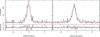 |
Fig. 1 Distance in RA and Dec between X-ray and infrared sources. There is a significant shift in declination between the two catalogues which we correct for before making the correlation. (This figure is available in color in electronic form.) |
We used the “likelihood ratio” method (Sutherland & Saunders 1992) to find the counterparts: we calculated the likelihood ratio (LR) of an infrared source to be a real counterpart of an X-ray source as

where q(m) is the expected magnitude distribution of real counterparts, f(x,y) is the probability distribution function of positional errors, a Gaussian in this case, and n(m) is the magnitude distribution of background objects. We calculate the q(m) function by subtracting the magnitude distribution of the background (IR) sources we expect to find within the search radius near the target (X-ray) sources from the magnitude distribution of all the initial counterparts. The normalization of q(m) is done using
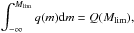
where Q(Mlim) is the probability that the IR counterpart is brighter than the magnitude limit Mlim; in practice it is the final fraction of X-ray sources with an IR counterpart. Given that the positional offsets of the X-ray sources in the CDFN at large off-axis angles can be as large as 1″ − 2″ (Alexander et al. 2003), we use a large initial search radius for the X-ray – IR counterparts (4″).
The choice of an optimum likelihood ratio cutoff is a compromise between the reliability of the final sample and its completeness. The reliability of a possible counterpart is defined as
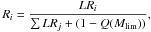
where j refers to the different IR counterparts to a specific X-ray source. We chose the likelihood-ratio cutoff, which maximizes the sum of completeness and reliability of the matched catalogue in the same manner as Luo et al. (2010). The completeness is defined as the ratio of the sum of the reliabilities of the counterparts with LR > LRlim with the number of the X-ray sources in the area mapped by IRAC, and the reliability is defined as the mean reliability of counterparts with LR > LRlim. In the X-ray – IR case LRlim = 0.15, which gives a reliability of 99.2%.
We detected 330 IR counterparts with LR > 0.15, then visually inspected the positions on the IRAC images of the X-ray sources lacking a counterpart and found 12 cases where the IR source is clearly visible but blended with a nearby source in a way that the source extraction algorithm could not distinguish them. Adding these cases, the final number of counterparts is 342 out of the 348 X-ray sources in the IRAC area. Assuming that 0.8% of the counterparts are spurious, the final efficiency is 97.5%.
In order to look for optical counterparts to the X-ray sources we used the positions of their IR counterparts. The positional accuracy of IRAC is better than that of Chandra, moreover the NIR is more efficient in detecting AGN than the optical emission, due to the reprocessing of the ionizing radiation of the AGN through circumnuclear and interstellar dust to IR wavelengths. As a result, the efficiency of IRAC in finding counterparts for the X-ray sources (97.5%) is higher than that of the optical survey (78.1% if we follow the procedure described above for the Subaru-R catalogue), in spite of the optical being deeper than IRAC (see also Luo et al. 2010, for the CDFS case).
The optical catalogue of Capak et al. (2004) has 47 450 sources detected in the R band, and of those 14 763 fall into the area sampled by IRAC. Before searching for optical counterparts, we again checked the relative astrometry of the optical and (uncorrected) IR catalogues. We again found a similar astrometry difference in the Dec axis ( ⟨ Dec(opt) − Dec(IR) ⟩ = − 0.22, σ = 0.20, Fig. 2), while the RA positions are well within the error ( ⟨ RA(opt) − RA(IR) ⟩ = 0.05, σ = 0.17). We again corrected the IR catalogue to match the optical positions.
We used the likelihood ratio method to select the optical counterparts to the IR sources. Given the smaller PSF of the optical images we uses a smaller initial search radius (3″) and followed the same procedure to select the optimum likelihood-ratio limit. With LRlim = 0.25, which this time gives a mean reliability of 98.4%, we found optical counterparts for 8437 of the 10 595 IRAC sources. The recovery rate is 78.0%. We also performed an independent search for optical counterparts of X-ray sources which do not have an infrared counterpart, or where the latter is a blended source as described above, and found a secure optical counterpart for 12 such cases; 11/12 of the “confused” IR sources have an optical source related to the X-ray position, while 1/6 of the IRAC non-detections is detected in optical. Finally, we optically inspected the Subaru R-band images of X-ray sources lacking an optical counterpart and found that in 17 the optical counterpart is clearly visible but without identification in the catalogue of Capak et al. (2004). Two common reasons for that are that the source is saturated, and therefore it does not have reliable photometry, and that it lies close to a very bright source and therefore it is not detected by the source-extracting algorithm.
The X-ray, optical, and infrared properties of all the sources of the common CDFN-IRAC area can be found in ftp.mpe.mpg.de/people/erovilos/CDFN_IR_OPT/
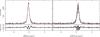 |
Fig. 2 Same as Fig. 1 but for the Spitzer (without including the correction introduced to match the X-ray astrometry) and optical catalogues. The shift in declination is again corrected for before correlating. (This figure is available in color in electronic form.) |
List of CDFN X-ray sources that are correlated with a Spitzer 3.6 μm detection and lack an optical counterpart in Capak et al. (2004).
3. Sample selection
In this study we are interested in X-ray sources which are too faint to be detected by typical ground-based optical surveys, like that of Capak et al. (2004). These sources represent a sizable fraction of the overall X-ray population (~15%). They are generally not covered by spectroscopic surveys, which are typically magnitude-limited with Rlim < 26.5 and often do not even have photometric redshifts. Such cases have been studied before in detail (e.g. Alexander et al. 2001; Mainieri et al. 2005); here we approach them using their infrared properties and X-ray spectra.
There are 310 X-ray sources within the common area of all the surveys used in this study (2 Ms CDFN – Subaru-Suprime(optical) – Subaru-MOIRCS(HK′) – GOODS-ACS – GOODS-IRAC – GOODS-MIPS). Of these 310 sources, 42 are too faint to be detected in the R-band by Subaru-Suprime and are assumed to have RAB > 26.5. No R-detected CDFN source has RAB > 26.5. Because we base this study on the infrared properties to examine the nature of optically faint sources, we excluded 7 of the 42 sources from our studied sample for the following reasons: 5 are not detected with IRAC, and 2 are blended with nearby sources, so their infrared photometry is not reliable. Our final sample consists of 35 sources, whose X-ray, optical, and infrared properties are listed in Table 1. Among these sources we expect a mean number of 0.35 spurious encounters (practically none), as the mean reliability of the IRAC counterparts for these 35 cases is 99.0%.
For these 35 sources we searched the KS catalogue of Bundy et al. (2009) for counterparts. These Subaru-MOIRCS images cover an area slightly smaller than IRAC, and we limited our field to the common area. As the number of sources is small, we looked for KS-band counterparts by eye; this way we can easily distinguish any KS-band sources that are physically related to a nearby IRAC source. We found a KS counterpart for 29/35 sources; their distances from the IRAC sources are all < 1.4″, while for the 6 non-detections the distance of the nearest KS source is always > 3.9″. We then searched the HK′-band images from the UH-2.2 m telescope (Capak et al. 2004) to detect any sources bright enough in the HK′ band but not detected in R. Using sextractor (Bertin & Arnouts 1996), we identify as a source 4 adjacent pixels with fluxes above 1.2 times the local background rms. We find an HK′ detection for 19 of the sources in our sample. The Subaru-MOIRCS area has very deep optical imaging with the HST-ACS as part of the GOODS survey. The catalogues (Giavalisco et al. 2004) are based on detections in the z850 band and are publicly available. We searched the sources of our sample for HST counterparts using the likelihood-ratio method, as described in the previous section, with an initial search radius of 1.5 arcsec. We use this method because the PSFs of Spitzer-IRAC and HST-ACS are different within a large factor and there could be multiple ACS sources within one IRAC beam. Of our sample 18/35 sources have an HST-ACS counterpart.
 |
Fig. 3 Cutout images of the sources listed in Table 1. In greyscale is the Subaru R-band from Capak et al. (2004). Large circles mark the positions of the X-ray sources with 4″ radii and contours represent the IRAC 3.6 μm flux. (This figure is available in color in electronic form.) |
We note here that some of the sources in Table 1 appear with full optical photometry in Barger et al. (2003a), some of them even with a photometric redshift. Where X-ray sources lack an optical counterpart, like the those in Table 1, Barger et al. (2003a) measured the optical fluxes directly from the Subaru images using a 3″ diameter aperture centred on the position of the X-ray source. In doing so there is a high probability that light from a neighbouring source enters the aperture, moreover centering on the X-ray positions causes a loss in positional accuracy, which is essential when measuring the flux of a “non-visible” source. Figure 3 shows the R-band images of the 35 sources of Table 1, with 4″-radii circles on the X-ray positions (as large as the initial search radius) as well as contours representing the IRAC flux. We can see that in some cases the X-ray and IRAC positions differ significantly and that the 1.5″ aperture centred on the X-ray position would often be contaminated by nearby optical sources.
The sample presented in Table 1 has both similarities and differences with the high X-ray-to-optical ratio sample (Civano et al. 2005) and the optically faint sample presented by Alexander et al. (2001). In Fig. 4 we plot the R magnitudes of the optical counterparts against the (0.5–8.0) keV flux as filled circles and the sources in our sample (all lower limits) as crosses. The shaded area is the log (fx/fopt) = 0 ± 1 area where the bulk of AGN are expected (e.g. Elvis et al. 1994). Our sources have, on average, a higher fx/fopt value than the bulk of the AGN population, but could not be securely considered as high fx/fopt (with a value > 10, Koekemoer et al. 2004). The HST V606 magnitudes provide a clearer picture. In Fig. 5 we plot the V606 magnitudes against the X-ray flux keeping the same symbols as in Fig. 4. The V606 magnitudes for non-detected sources are assumed to be V606 > 27.8, the same as the detection threshold in the z580 band. The true limits however are likely to be higher, as the typical V606 − z850 colour of AGN hosts is > 0.5 and increasing with redshift (Sánchez et al. 2004); the 2σ limits of sources 246 and 317, which are detected in the z580 band and not in the V606 band, are 29.6 and 29.9 respectively. In Fig. 5 we see that the sources of Table 1 are clearly relatively high fx/fopt, all having log (fx/fopt) > 0.52. However, compared to Civano et al. (2005), this is neither fully a high fx/fopt sample, nor a complete one, as many sources with log (fx/fopt) > 1 are not included. Moreover, the high fx/fopt sample of Civano et al. (2005) includes much brighter sources, as bright as R ~ 23.
Compared to Alexander et al. (2001), our sample probes much fainter sources; the Alexander et al. (2001) sample has a cut at I = 24. As a result, their sources have relatively low X-ray-to-optical flux ratios, in many cases log (fx/fopt) < 0.
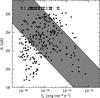 |
Fig. 4 Optical versus X-ray flux for all the X-ray sources in the common area (see text). Crosses mark the sources of Table 1 and the shaded area marks log (fx/fopt) = 0 ± 1 where the bulk of AGN are expected. |
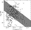 |
Fig. 5 Same as Fig. 4 but for the HST-ACS V606 optical flux. The V606 > 27.8 upper limit for non-detection is likely to be an under-estimation (see text). |
4. Photometric redshifts
We use the EAZY code (Brammer et al. 2008) to calculate photometric redshifts. We used 4 ACS (B435, V606, i775, and z850) optical, HK′ (when available), KS and 2 IRAC bands (3.6 μm, 4.5 μm) to constrain the photometric redshifts. We do not use the 5.8 μm and 8.0 μm bands because they are more sensitive to the properties of (interstellar and circumnuclear in AGN cases like here) dust, something which would add extra parameters that would have to be considered in the template fitting (see Rowan-Robinson et al. 2008).
The results are also shown in Table 1; the HST magnitudes shown as lower limit are detections with a < 2σ confidence in the respective bands, and the 2σ flux is used to calculate the magnitude. The photometric redshifts based on these lower limits are considered less reliable. Note that source 369, despite being very faint in the optical, has a reported spectroscopic redshift of z = 2.914 in Chapman et al. (2005). The position of the spectroscopic source comes from the radio (VLA – 1.4 GHz) catalogue of Richards (2000) and agrees within 0.15″ with the IRAC position. The spectrum is typical of an AGN (CIV line) and the X-ray position is 1.1″ away, so we are confident that this is the correct counterpart. The photometric redshift derived by EAZY (2.80) is close to the spectroscopic value.
For sources without ACS detection, it is very challenging to derive a photometric redshift based only on the IRAC and KS bands. In these cases we are forced to use all IRAC bands, which adds the extra variable of the dust properties. A good example of poor photo-z accuracy in cases where only mid-infrared fluxes are fitted can be found in Salvato et al. (2009). The redshift derived is typically 2 < z < 3, but the constrain is weak and the broad-band spectrum in some cases can be equally well fitted with SEDs shifted to z > 3.2. The reason for that is that in cases where the IRAC SEDs are monotonic in fν the fit cannot be easily constrained. A good photo-z estimate with a value of z ~ 2.5 is derived for a blue [5.8]–[8.0] colour1, which can be fitted with the red-NIR bump of a galactic (no AGN) SED due to moderate temperature interstellar gas (see Fig. 8 in Salvato et al. 2009). From Table 1, we can see that of the 14 sources with full IRAC photometry and no ACS detection, 5 have blue [5.8]–[8.0] colour (98, 140, 156, 198, and 372). The median photometric redshift for these five sources as derived by EAZY is z = 2.39, whereas the median photo-z for the red [5.8]–[8.0] colours is z = 4.40. The two samples define different populations in terms of photometric redshifts with a confidence level of 99.5%, according to a K-S test. Moreover, the “HST-detections” and “HST-non-detections” populations are also different within 98.9%, having median redshifts 2.61 and 3.48 respectively.
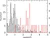 |
Fig. 6 Redshift distributions of CDFN sources in the common CDFN-GOODS-MOIRCS area. The black histogram represents all optically detected sources with the shaded histogram representing spectroscopic redshifts. The red histogram (referring to the right axis scale) represents the optically faint sources. (This figure is available in color in electronic form.) |
The redshift distribution of the sources in Table 1 is compared with the distribution of all X-ray sources in the common CDFN-GOODS-MOIRCS in Fig. 6. The black histogram represents all optically detected sources and the shaded histogram represents sources with spectroscopic redshifts, taken from the catalogues of Barger et al. (2003a) and Trouille et al. (2008). The red histogram (referring to the right axis scale) represents the sources of Table 1. The two distributions are remarkedly different, with the sources of Table 1 being at higher redshifts.
5. X-ray spectral analysis
The data were analysed using the CIAO v.4.1 analysis software. The source spectra were extracted from circular regions with variable radii so as to include at least 90 per cent of the source photons in all off-axis angles. There are 20 X-ray observations comprising the total ~2 Ms exposure. We extracted the source spectrum and auxiliary files for each observation separately using the CIAO SPECEXTRACT script. Then we used the MATHPHA ADDARF and ADDRMF tasks of FTOOLS to merge the spectral products for each source. The background files were calculated from source-free regions in each observation and are again merged using the MATHPHA tool.
We explored the X-ray properties of the 35 sources in our sample using the XSPEC v12.5 package to perform X-ray spectral fittings. For the sources with adequate count statistics (net source counts ≥ 200, 5 sources), we used the χ2 statistic technique. The data were grouped to give a minimum of 15 counts per bin to ensure that Gaussian statistics apply. We adopted an absorbed power-law model and attempted to constrain the intrinsic absorption column density NH (i.e., after having subtracted the Galactic absorption) and the power-law photon index Γ.
X-ray properties.
For the sources with limited photon statistics (net counts < 200), we used the C-statistic technique (Cash 1979), which is specifically developed to extract spectral information from data with a low signal-to-noise ratio. In this case, the data are grouped to give a minimum of one count per bin to avoid zero count bins. We tried to constrain the intrinsic column densities using an absorbed power-law model with Γ fixed to 1.8. In both cases, the spectral fittings are performed in the 0.3–8 keV energy band where the sensitivity of the Chandra detector is the highest. The estimated errors correspond to the 90 per cent confidence level. In Table 2 we present the spectral fitting results for the 35 sources comprising our final dataset. Source 107 has a very flat photon index, which is likely to be the result of a reflection-dominated spectrum (see Georgantopoulos et al. 2009, for a detailed analysis of the candidate Compton-thick sources in the CDFN). In this case the hydrogen column density in Table 2 is not correct, and the true NH of the source is > 1024 cm-2. There are two more Compton-thick sources (199 and 369) in our sample that are transmission dominated. In these the X-ray-absorption turnover is redshifted at low energies (5 − 6 keV) and an observer’s frame NH ~ 3 × 1023 cm-2 is measured, which yields a rest-frame NH > 1024 cm-2 when the (1 + z)2.65 correction is applied. The most secure Compton-thick source is 369, for which there is spectroscopic redshift available and therefore a more reliable determination of the rest-frame column density. Note that this source is not included in the CDFN Compton-thick sample of Georgantopoulos et al. (2009), because it has a flux lower than their adopted flux limit of 10-15 erg cm-2 s-1 in the 2–10 keV band.
Next, we compared the mean X-ray spectral indices by coadding the individual X-ray spectra in the total 0.3–8 keV band for four different sets of sources (see Table 3). We fitted a simple power-law model to the data. It is evident that our sources present a very hard X-ray spectrum. The total spectrum of all 35 sources has Γ ≈ 0.9, which is harder than the coadded spectrum of all the detected X-ray sources in this band (Γ = 1.4, Tozzi et al. 2001). Note that the derived mean spectrum is comparable to the spectrum derived by Fiore et al. (2008) and Georgantopoulos et al. (2008) for dust obscured galaxies, i.e. sources defined as having f24 μm/fR > 1000; the coadded spectrum of DOGs in our sample has Γ = 1.05. The sources with IRAC-only detections are significantly harder than those with optical HST counterparts. This difference cannot be attributed to the fact that they have on average different redshifts and hence different K-corrections, as it would work in the opposite case. The HST-detected sources are intrinsically softer than the ones completely lacking an optical counterpart.
6. Optical properties
In Fig. 7 we plot the V606 − i775 vs. i775 − z850 colours of the 18 sources in our sample which have an ACS detection. Red points mark the objects of our sample and black dots are HST sources associated with an X-ray source. All the HST detections are shown in comparison as blue points. The open circle with the right arrow represents source 317, which has a low significance ( < 2σ) detection in the V606 and i775 bands, and its V606 − i775 colour cannot be accurately determined. The coloured lines in Fig. 7 trace the colours of various templates with redshift with points marking z = 0,1,2,3. The templates are the Coleman et al. (1980) galaxy templates for elliptical, spiral, and irregular galaxies. Dotted lines correspond to z > 4, where the blue edge of the V606 filter is redshifted to the Lyman break (912 Å). The templates used are zeroed at shorter wavelengths than the Lyman break, so the dotted lines are approximations of the colours at high redshift. The sources of our sample appear significantly redder than the overall X-ray population; 55.6% (10/18) of them have i775 − z850 > 0.8 compared to 14.4% (42/291) of the overall X-ray population; the probability that the i775 − z850 colours of the red points are a random sample of the black points in Fig. 7 is < 0.01%. The colours of the red objects appear to be consistent with the elliptical template at z = 2 ± 1, which is backed up by the photometric redshifts of Table 1. Red optical colours are often associated with early-type morphologies (see Bell et al. 2004).
In Fig. 8 we plot the HST-ACS cutouts of the galaxies of Table 1. Each thumbnail is a combination of the four ACS (B − V − i − z) images to increase the signal-to-noise ratio, and the contours represent the IRAC 3.6 μm flux, as in Fig. 3. The crosses mark the positions of the HST sources with an inner radius of 0.5″ and an outer radius of 2″. We can see that for sources recovered with the HST the morphologies cannot be determined.
Based on their near-infrared (KS) to optical colours, many of the sources in our sample are associated with extremely red objects (EROs; Elston et al. 1988). They are usually defined as galaxies with R − K > 5 (see also Alexander et al. 2002, for a selection based on the I-band with I − K > 4). If we use the R-band limit (RAB > 26.5 ⇒ RVega > 26.3), 13/29 of the sources detected in KS are EROs. However, the true optical flux of the sources is fainter than this limit; if we use the V606 ACS magnitude for HST-detected sources and VAB > 27.8 ⇒ VVega > 27.722, 28/29 of the KS detections have V606 − KS > 5. Source 335 has V606 − KS > 4.86 and it is not detected with the HST, so it is highly probable that it too is an ERO. Of the six sources not detected in KS, 100, 151, 250, 329 and 374 are not detected with the HST either, so they could be associated with EROs and 181 has V606 − KS < 5.03. Morphologically, EROs are a mix of early and late-type systems (Cimatti et al. 2003; Gilbank et al. 2003), and those with higher redshift tend to be more late-type (Moustakas et al. 2004).
Co-added X-ray spectral properties.
7. Infrared properties
We plot the mid-infrared colours of the sources of Table 1 in Fig. 9. This diagram has been used by Stern et al. (2005) to select AGN by their mid-infrared colours; a high fraction (up to 90%) of broad-line AGN is located inside the “wedge” marked with the black solid line in Fig. 9. The HST-detected and non-detected sources of Table 1 are plotted with filled and open circles respectively. The coloured lines represent the colours of the Coleman et al. (1980) galaxy templates as well as a QSO SED (Elvis et al. 1994) for 0 < z < 8, and point marks z = 0,1,2,3,4,5,6,7.
The sources of Table 1 are located both inside and outside the wedge in Fig. 9, in the area where the red/optically-faint mid-IR AGN of Georgantopoulos et al. (2008) lie. There is a separation in the colours of HST detections and non-detections, the latter population with mid-infrared colours mostly inside the wedge (10/14), and the rest being equally distributed (9/18). This difference reflects on their [5.8]–[8.0] colours, a K-S test shows that HST detections have bluer [5.8]–[8.0] colours than non-detections with 99.0% (2.6σ) significance, and this is what causes the photometric redshifts of HST non-detections to be higher. The galaxy templates of Coleman et al. (1980) enter the wedge at z = 3 so the photometric redshift of those sources is z > 3 if they are fitted with those templates. However, the QSO template is in the wedge independent of the redshift because of its power-law shape; indeed this is the reason why this diagram is a selection method for mid-infrared AGN. So, a red [5.8]–[8.0] colour and the position inside the wedge can be explained either with a QSO SED or a high-redshift (z > 3) galaxy SED.
 |
Fig. 7 Optical colours of HST-detected sources. The optically faint sources of Table 1 appear in red and the X-ray sources appear in black. For comparison, all HST sources of Giavalisco et al. (2004) are plotted in blue. Colour lines track the colours of the Coleman et al. (1980) SED templates with redshift. (This figure is available in color in electronic form.) |
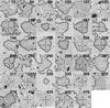 |
Fig. 8 HST cutouts of all sources listed in Table 1. The images are combinations of the four ACS bands available to increase the signal-to-noise ratio, the contours represent the IRAC flux, and the crosses are centred on the GOODS source positions (if any) with an inner radius of 0.5″ and an outer radius of 2″. |
8. Discussion
8.1. High or intermediate-z sources ?
In an earlier study of optically faint sources in the CDFN, Alexander et al. (2001) concluded that they are moderately obscured AGN at redshifts z = 1 − 3, leaving a small margin for very high redshift QSOs in the optically fainter subsample. However, their modest optical magnitude cutoff (I > 24) includes sources that have “normal” X-ray to optical ratios (fx/fopt ~ 1). Studying more extreme cases based on fainter optical fluxes or higher X-ray to optical ratios, Barger et al. (2003b) and Koekemoer et al. (2004) suggest that the existence of very high redshift objects cannot be definitely ruled out. In this study we compose a sample of the optically faintest AGN (R > 26.5) with robust infrared identifications which is 83.3% complete, including 35 of the 42 R > 26.5 X-ray sources in the common CDFN-GOODS-MOIRCS area used.
8.1.1. Multi-λ investigation
For the 18 sources with an HST identification we calculated their photometric redshifts using up to eight optical and infrared bands, and the results show that they are indeed at moderate redshifts, with a median z = 2.61, while all have z < 3.65. The redshift of the remaining 17 sources without optical HST is harder to constrain, and we attempted to derive photometric redshifts using the infrared bands. The redshifts for sources with mid-infrared colours outside the “wedge” of Fig. 9, or alternatively with fν5.8 μm > fν8.0 μm (six sources) can be better constrained, they have a median redshift of z = 2.39. We assume that in these cases the host galaxy dominates the mid-infrared colours, which are well fitted with non-AGN SEDs at 2 < z < 3 (green, cyan, yellow, and magenta lines in Fig. 9). The nine sources without optical HST detection and fν5.8 μm < fν8.0 μm have mid-infrared colours compatible both with normal galaxy (or host galaxy) templates at high redshifts or with QSO templates without a strong redshift constraint (see Sect. 4); we tried to constrain their redshifts using photometry from lower energy infrared bands (24 μm, see Soifer et al. 2008).
The position of the QSO templates inside the wedge is the result of the heating of the circumnuclear dust with the radiation of the AGN, which results in a red power-law SED (fν ∝ ν − α with α < − 0.5). The circumnuclear dust can also extinguish the optical emission; Dunlop et al. (2007) claim that optically faint sources can be well fitted with dusty and extremely reddened (AV ≃ 4) SEDs at moderate redshifts (z ~ 2.5). We therefore check the mid-infrared 24 μm emission of the sources of our sample to examine the dust properties. Of the 17 sources without HST detection, seven are detected by MIPS, including 5/9 sources with fν5.8 μm < fν8.0 μm. In Fig. 10 we plot the 24 μm emission in comparison with the 3.6 μm emission. As dots we plot the overall population (non-AGN), as crosses we plot the counterparts of the X-ray sources (AGN) and as black filled and red open circles we plot the optically faint sources with and without an HST detection respectively. We can see that the optically faint sources are in general fainter in 3.6 μm emission with respect to their 24 μm emission, which indicates dust extinction of optical and near-infrared wavelengths, unless there is a strong 24 μm component from the AGN. The 24 μm emission upper limits of the HST non-detections can in most cases be explained with dust obscuration, in cases where f3.6 μm < 5 μJy. The harder X-ray spectra of the HST non-detections also suggest that (despite their somewhat higher redshifts) these sources are more obscured, and this is what causes the faint optical fluxes.
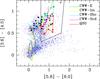 |
Fig. 9 Infrared colours of the sources listed in Table 1. HST-detected sources are plotted in filled circles and HST non-detections in open circles. All 3.6 μm detected sources are plotted in blue dots. The colour lines track the colours of the Coleman et al. (1980) SED templates with redshift and the black lines mark the region where infrared-selected AGN are located (Stern et al. 2005). (This figure is available in color in electronic form.) |
The four sources without HST detection, f5.8μm < f8.0μm, and no 24μm detection (84, 151, 204, and 335) are possibly associated with high-redshift objects. However, the 24μm upper limits of three of them (151, 204, and 335) do not rule out dust obscuration given their low 3.6μm fluxes ( < 3.6μJy). Source 84 with f3.6μm = 6.546μJy has an f3.6μm/f24μm ratio lower limit similar to the overall AGN population without clear signs of dust absorption and is therefore a high-redshift candidate. Its photometric redshift based on the 4 IRAC bands (4.50) is weakly constrained and not reliable.
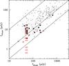 |
Fig. 10 3.6 μmvs. 24 μm emission. Dots represent the overall 3.6 μm population with a 24μm counterpart, crosses the counterparts of X-ray sources, black filled circles the sources of Table 1 detected with the HST and red open circles the sources of Table 1 not detected with the HST. The lines mark log (f3.6μm/f24μm) = 0, − 1, − 1.5. (This figure is available in color in electronic form.) |
8.1.2. Dropouts
The Lyman-break technique (e.g. Steidel et al. 2003) is often used to select high-redshift objects, and is based on the sudden drop in the flux of the broad-band spectrum at wavelengths smaller than 912 Å. Lehmer et al. (2005) used the HST observations to search for dropout sources among the z850-detected sources in the CDFN. They found two V606-dropouts at z ≳ 5 and one i775-dropout at z ≳ 6. One of the two V606-dropouts (source 247 in Alexander et al. 2003) is not included in Table 1 because it is near a brighter optical source (1.6 arcsec separation) and the two are blended in the IRAC image. It has a spectroscopically confirmed redshift of z = 5.186 (Barger et al. 2003a). The other V606-dropout (source 246) has a red i775 − z850 colour (1.1), like most of the sources in the HST-detected sample, and its V606 − i775 colour is a lower limit (V606 − i775 > 1.275 if we take the V606 2σ limit), which is compatible both with early-type templates at z ~ 1.5 and with very high redshift late-type templates, depending on the true V606 − i775 colour. This source is also observed spectroscopically, but neither a redshift nor a spectral type could be derived (Barger et al. 2003a; Trouille et al. 2008). It has no MIPS 24μm detection, but its mid-infrared colours ( [ 5.8 ] − [ 8.0 ] = 0.265) argue against a high redshift, they are explained by normal galaxy templates with 2 < z < 3, agreeing with the photometric redshift (2.80) derived using seven optical and infrared bands.
The i775-dropout of Lehmer et al. (2005) is source 317. Its photometric redshift (3.25) is based on lower significance B435, V606, and i775 measurements and it is not reliable. This the source with the highest 24μm flux in our sample (f24μm = 664μJy), which would yield a mid-infrared luminosity of the order of 1026WHz-1 in the 3.5μm rest-frame band if the source were lying at z ~ 6. Its low f3.6μm/f24μm ratio however (10-1.1) implies dust obscuration according to Fig. 10, making it more likely to be optically faint as a result of obscurarion rather than high redshift.
The dropout technique is proposed to select high-redshift objects, but it is based in 2–3 bands, usually including upper limits. All sources in our sample are “optical dropouts” in the sense that they are not detected in wavelengths shorter than a limit, in this case the R-band optical, and taking the HST observations into account, almost half of them are z-dropouts. When considering their multi-band properties however we see that a small fraction of them (if any) can be high-redshift (z ≳ 6) sources, as there are other processes which can cause the faint optical fluxes. Because the SEDs are a combination of the AGN and the host galaxy, a simple colour selection could be misleading in our examination of AGN-hosting systems
8.2. Obscured AGN?
The colour-colour diagram of Fig. 7 shows that the sources that are detected by the HST have on average redder optical colours than the overall X-ray population and are compatible with elliptical galaxy SEDs. Rovilos & Georgantopoulos (2007) and Georgakakis et al. (2008) have shown that red-cloud AGN are obscured post-starburst systems. Instead, Brusa et al. (2009) attribute the red colours to dust-reddening rather than to an evolved stellar population. It is still true though that X-ray AGN with red optical colours have a high fraction of obscured sources.
A number of studies (e.g. Alexander et al. 2001; Mignoli et al. 2004; Koekemoer et al. 2004) relate high X-ray-to-optical ratios to the extremely red objects sample, with R − K > 5. The sources of Table 1 have by definition high X-ray-to-optical ratios. Using the HST magnitudes, we get log (fx/fopt) > 0.52 between the ACS-V band (λeff = 6060Å) and the (0.5–10) keV X-ray band, assuming an optical limit V606 > 27.8(AB) for non detected sources (see Sect. 3 and Fig. 5). They also have very red colours with V606 − KS > 5. X-ray detected EROs are assumed to be low-Eddington obscured AGN and they show on average high fx/fopt values (Brusa et al. 2005), like our sources. The HST-detected subsample, which shows red optical colours, has similar characteristics to the high X/O EROs of Mignoli et al. (2004), although this is a much fainter sample. Their sample is detected in the K-band and has bulge-dominated morphologies, dominated by their host galaxies (see also Maiolino et al. 2006).
The sources in our sample are selected to have faint optical fluxes, and thus naturally many of them are associated with DOGs. They are found at a redshift of z ≃ 2 (e.g. Pope et al. 2008) and are thought to be marking a phase of bulge and black-hole growth. Hydrodynamic simulations (Narayanan et al. 2010) suggest that DOGs are rapidly evolving from starburst to AGN-dominated systems through mergers in cases where fν(24μm) ≳ 300μJy. Alternatively, in cases where fν(24μm) ≲ 300μJy the evolution is secular, that is through smaller gravitational perturbations. Their morphological characteristics (Melbourne et al. 2009) reveal less concentrated systems for lower luminosities.
Considering the V606 magnitudes, and a V606 > 27.8 in cases of HST non-detections, all objects in Table 1 with a MIPS detection (17/35 sources) have DOG characteristics3, and based on 24μm upper limits the rest are not incompatible with DOGs, as the fν(24μm)/fν(V606) upper limit is always > 1250. Therefore half of our sample have characteristics consistent with DOGs and this is only a lower limit. Only one source (317) has fν(24μm) > 300μJy. Their red optical colours (HST detections) suggest early-type bulge-dominated morphologies (Bell et al. 2004; Mignoli et al. 2004), although the morphologies cannot be determined from direct observations, which is in line with their low 24μm fluxes (see also Bussmann et al. 2009). In conjunction with the obscured nature of the AGN, this means that the host galaxy is dominating the optical light.
On the basis of an X-ray stacking analysis in deep X-ray fields, Fiore et al. (2008, 2009); )Treister et al. (2009) propose that DOGs may be hosting a large fraction of Compton-thick sources (see also Georgantopoulos et al. 2008). The sources of our sample appear to be more obscured than the overall X-ray population, the average spectral index being Γ = 0.87 compared to Γ = 1.4 (Tozzi et al. 2001). The stacked spectrum of X-ray detected DOGs in the Chandra deep fields is Γ ≃ 0.7 (Georgantopoulos et al. 2008), comparable to those of our total and DOG samples. The average Γ of our DOG sample is very close to the value derived by Georgantopoulos et al. (2010, submitted) using all DOGs in the CDFN regardless of their optical detection (or lack of it), a sample broadly overlapping with ours.
According to Table 2, the average column density is a few times 1023 cm-2. A few Compton-thick AGN may be also present in our sample, this includes the reflection-dominated source (107; see Georgantopoulos et al. 2009). Two more “mildly” Compton-thick sources, i.e. with column densities NH ~ 1024 cm-2, are directly identified on the basis of their absorption turnover entering the Chandra passband. Finally, we note that a number of our sources (10/35) of Table 2 have unobscured hard X-ray luminosities Lx > 1044ergs-1 and intrinsic NH > 1023cm-2, making them members of the QSO2 class. It is interesting that these sources do not reveal their QSO nature except in X-rays.
8.3. X-ray luminosity function incompleteness
In the CDFs a number of X-ray sources lack an optical counterpart, even in the deepest ground-based optical surveys. More specifically, within the common CDFN – GOODS – MOIRCS area there are 35 sources which are not detected at a magnitude limit of R ~ 26.5 and 17 sources not detected at z850 ~ 27.8. These populations represent 11.3% and 5.5% of the X-ray population detected in this area. These numbers should be considered as lower limits, as there are seven other X-ray sources without optical counterpart not included in Table 1 because either they are not detected with Spitzer or have unreliable photometry. Moreover, there is a number of stars, normal galaxies, or ultraluminous X-ray sources (Hornschemeier et al. 2003; Bauer et al. 2004) among the 310 X-ray sources, so the fraction of non-optically identified X-ray AGN is even higher.
This sample of optically faint X-ray sources is not random in their redshift distribution; the redshifts calculated in Sect. 4 and the K-S test performed show that the optically faint X-ray sources have significantly higher redshifts than the overall population and the HST non-detections higher again. The redshifts listed in Table 1 are in 34/35 cases higher than 1.5. There are 41 sources if we count the sources within the common GOODS – IRAC – MOIRCS area with an optical detection in Capak et al. (2004) and z > 1.5. This means that the incompleteness of the X-ray z > 1.5 population with an optical identification and a redshift estimation is ~ 50% and it becomes even higher at higher redshifts; 29/35 of our sources have z > 2.
This has implications in the calculation of the X-ray luminosity function at high redshift (z > 2 − 4) and its evolution (e.g. Silverman et al. 2008; Aird et al. 2008; Yencho et al. 2009; Aird et al. 2010). More specifically, this incompleteness affects the faint end of the XLF, as its “knee” at z = 2 is at log Lx ~ 44.5 ergs-1 (log L* = 44.4 − 45.0ergs-1 depending on the luminosity evolution model, Silverman et al. 2008; Aird et al. 2010), and 34/35 of the sources in Table 2 have unobscured X-ray luminosities Lx < 1044.5 ergs-1 in the 2 − 8 keV band.
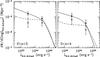 |
Fig. 11 Space density of AGN in the CDFN in two redshift bins (2 < z < 3, left, and 3 < z < 4, right) and two luminosity bins (1043 < L2.0 − 8.0keV < 1044, and 1044 < L2.0 − 8.0keV < 1045), without correction applied for optical non-detections. Open symbols are based on the sources in the CDFN – GOODS – MOIRCS area with a redshift determination in Barger et al. (2003a) and Trouille et al. (2008) and filled symbols are based on the combination of those sources with those of Table 1. The solid and dashed lines represent the best-fit mod-PLE and LDDE models respectively (see Silverman et al. 2008). |
In order to test how the inclusion of the sources in Table 1 affects the luminosity function at high redshift, we calculate the luminosity function of AGN in two redshift bins, 2 < z < 3, and 3 < z < 4, with and without their contribution, using the method described by Page & Carrera (2000). We used the combination of the CDFN catalogues of Barger et al. (2003a) and Trouille et al. (2008) and selected sources in the combined CDFN – GOODS – MOIRCS area. We did not make any distinction between spectroscopic and photometric redshifts and we do not correct for optically unidentified sources. This has an effect on the derived luminosity function only when we do not include the sources of Table 1, as the final sample is nearly complete.
The result is plotted in Fig. 11. We can see that the inclusion of the new sources severely affects the calculated luminosity function. We note that in most cases in the literature the incompleteness caused by optically non-detected sources is treated by either taking an optically bright sample which is spectroscopically complete, with the side effect of undersampling the high redshift – low luminosity cases (e.g. Yencho et al. 2009), or using simplistic assumptions, like that their redshift distribution is directly connected to their X-ray flux (e.g. Silverman et al. 2008), which is generally not true, or treating the incompleteness as a free parameter when fitting the datapoints to determine the luminosity function evolution (e.g. Aird et al. 2010). In Fig. 11 we also compare our datapoints with models of AGN evolution, which we adopt from Silverman et al. (2008). These are a modified pure luminosity evolution (mod-PLE) model (see Hopkins et al. 2007) (solid line) and a luminosity-dependent density evolution (LDDE) model (dashed line). Our datapoints are remarkably close to the prediction of the mod-PLE model, while the non-corrected points are closer to those of the LDDE model. A thorough investigation of the luminosity function evolution however would require taking into account sources at all redshifts and luminosities, which would vastly increase the reliability of the statistics. This analysis is beyond the scope of this work, but we caution that the optically faint sources, despite being a small minority of the X-ray sources, can impact the LF in high redshifts because of their redshift distribution.
9. Conclusions
We have examined the mid-IR and X-ray properties of 35 X-ray-selected sources in the GOODS-N area that are optically faint (RAB > 26.5) and therefore missed in ground-based optical observations. Instead of relying on previous work on the matching between X-ray and optical counterparts, our sample has been compiled anew. We found secure 3.6 μm counterparts for the X-ray sources using a likelihood-ratio technique, and then we searched for their possible optical ground-based RAB counterparts. Where there were none down to RAB = 26.5, we searched for HST ACS optical counterparts. Eighteen sources have HST counterparts, while the remaining have no optical counterparts. Our findings can be summarized as follows:
-
1.
Our sources populate moderate to high redshifts, while they areat markedly different redshifts from the alreadyspectroscopically identified population, which peaks atz ~ 0.7. In particular, the redshifts of the AGN with HST detections have moderate values with a median redshift of 2.6. The redshifts of the sources with IRAC detections only are definitely more uncertain; the objects with blue [5.8]–[8.0] colours are probably located at redshifts comparable with the HST population, z ~ 2.5, while the remaining sources could lie at z ≳ 3.2. A couple of V and i dropouts exist in our sample (previously reported by Lehmer et al. 2005), we however propose that they are moderate redshift (z = 2 − 3) dust-extinguished AGN, rather than lying at very high redshift (z > 5).
-
2.
The sources without optical counterparts in deep ground-based optical surveys constitute a large fraction ( > 50%) of the total source population at high redshift (z > 2). This has important implications for the calculation and modelling of the luminosity function at high redshift, which in the case of our highly complete sample (97% of the X-ray sources have spectroscopic or photometric redshifts) is better represented by a modified PLE model.
-
3.
Our sources present very red colours. In particular, all 35 sources with available KS magnitudes would be characterized as EROs on the basis of their V606 − KS colour.
-
4.
The mid-IR colours of the sources with HST counterparts lie outside the AGN wedge in a region occupied by z ~ 2 galaxies according to the galaxy templates, and have blue [5.8]–[8.0] colours. The majority Spitzer IRAC mid-IR colours of the remaining sources without optical counterparts lie within the AGN “wedge”, suggesting either QSO templates or galaxy templates at high redshift (z > 3).
-
5.
We find four high-redshift candidates based on their non-detection with the HST, red [ 5.8 ] − [ 8.0 ] colour, and non-detection with MIPS at 24μm. However, the low IRAC 3.6μm of three of them do not definately rule out dust obscuration in optical wavelengths.
-
6.
Seventeen out of 35 sources are detected in 24μm and can be classified as optically faint mid-IR bright galaxies. This class of objects is widely believed to consist of reddened sources at moderate (~2) redshifts.
-
7.
The mean X-ray spectrum of our sources is very hard with Γ ≈ 0.9, much harder than the spectrum of all sources in the CDFs, suggesting that we are viewing heavily obscured sources. The X-ray spectroscopy of the individual sources suggests that three sources are candidate Compton-thick AGN.
Obviously the current deepest X-ray observations are not at par with the present day optical spectroscopic capabilities. Spitzer has detected the faintest X-ray sources and thus provided aid in the determination of their properties and photometric redshifts.
We define here blue as fν5.8 μm > fν8.0 μm, corresponding to [ 5.8 ] − [ 8.0 ] < 0.64
The detection limit in the z850 ACS band is 27.8(AB) and according to the colours of HST detections the V606 limit is expected to be even higher.
They all have fν(24μm)/fν(V606) > 1000, except source 196 with fν(24μm)/fν(V606) > 890.
Acknowledgments
I.G. acknowledges the receipt of a Marie Curie Fellowship Grant. The data used here have been obtained from the Chandra X-ray archive, the NASA/IPAC Infrared Science Archive and the MAST multimission archive at StScI.
References
- Aird, J., Nandra, K., Georgakakis, A., Laird, E. S., et al. 2008, MNRAS, 387, 883 [NASA ADS] [CrossRef] [Google Scholar]
- Aird, J., Nandra, K., Laird, E. S., et al. 2010, MNRAS, 401, 2531 [NASA ADS] [CrossRef] [Google Scholar]
- Alexander, D. M., Brandt, W. N., Hornschemeier, A. E., et al. 2001, AJ, 122, 2156 [NASA ADS] [CrossRef] [Google Scholar]
- Alexander, D. M., Vignali, C., Bauer, F. E., et al. 2002, AJ, 123, 1149 [NASA ADS] [CrossRef] [Google Scholar]
- Alexander, D. M., Bauer, F. E., Brandt, W. N., et al. 2003, AJ, 126, 539 [NASA ADS] [CrossRef] [Google Scholar]
- Barger, A. J., Cowie, L. L., Capak, P., et al. 2003a, AJ, 126, 632 [NASA ADS] [CrossRef] [Google Scholar]
- Barger, A. J., Cowie, L. L., Capak, P., et al. 2003b, ApJ, 584, L61 [NASA ADS] [CrossRef] [Google Scholar]
- Bauer, F. E., Alexander, D. M., Brandt, W. N., et al. 2004, AJ, 128, 2048 [NASA ADS] [CrossRef] [Google Scholar]
- Bell, E. F., McIntosh, D. H., Barden, M., et al. 2004, ApJ, 600L, 11 [Google Scholar]
- Bertin, E., & Arnouts, S. 1996, A&AS, 117, 393 [NASA ADS] [CrossRef] [EDP Sciences] [Google Scholar]
- Brandt, W. N., & Hasinger, G. 2005, ARA&A, 43, 827 [Google Scholar]
- Bundy, K., Fukugita, M., Ellis, R. S., et al. 2009, ApJ, 697, 1369 [NASA ADS] [CrossRef] [Google Scholar]
- Bussmann, R. S., Dey, A., Lotz, J., et al. 2009, ApJ, 693, 750 [NASA ADS] [CrossRef] [Google Scholar]
- Brammer, G. B., van Dokkum, P. G., & Coppi, P. 2008, ApJ, 686, 1503 [NASA ADS] [CrossRef] [Google Scholar]
- Brusa, M., Comastri, A., Daddi, E., et al. 2005, A&A, 432, 69 [NASA ADS] [CrossRef] [EDP Sciences] [Google Scholar]
- Brusa, M., Fiore, F., Santini, P., et al. 2009, A&A, 507, 1277 [NASA ADS] [CrossRef] [EDP Sciences] [Google Scholar]
- Capak, P., Cowie, L. L., Hu, E. M., et al. 2004, AJ, 127, 180 [NASA ADS] [CrossRef] [Google Scholar]
- Cash, W. 1979, ApJ, 228, 939 [NASA ADS] [CrossRef] [Google Scholar]
- Chapman, S. C., Blain, A. W., Smail, I., & Ivison, R. J. 2005, ApJ, 622, 772 [NASA ADS] [CrossRef] [Google Scholar]
- Ciliegi, P., Zamorani, G., Hasinger, G., et al. 2003, A&A, 398, 901 [NASA ADS] [CrossRef] [EDP Sciences] [Google Scholar]
- Civano, F., Comastri, A., & Brusa, M. 2005, MNRAS, 358, 693 [NASA ADS] [CrossRef] [Google Scholar]
- Cimatti, A., Daddi, E., Cassata, P., et al. 2003, A&A, 412, L1 [NASA ADS] [CrossRef] [EDP Sciences] [Google Scholar]
- Coleman, G. D., Wu, C.-C., & Weedman, D. W. 1980, ApJS, 43, 393 [NASA ADS] [CrossRef] [Google Scholar]
- Dickinson, M. 2004, BAAS, 36, 1614 [NASA ADS] [Google Scholar]
- Giavalisco, M., Ferguson, H. C., Koekemoer, A. M., et al. 2004, ApJ, 600, L93 [NASA ADS] [CrossRef] [Google Scholar]
- Gilbank, D. G., Smail, I., Ivison, R. J., & Packham, C. 2003, MNRAS, 346, 1125 [NASA ADS] [CrossRef] [Google Scholar]
- Daddi, E., Alexander, D. M., Dickinson, M., et al. 2007, ApJ, 670, 173 [NASA ADS] [CrossRef] [Google Scholar]
- Dey, A., Soifer, B. T., Desai, V., et al. 2008, ApJ, 677, 956 [Google Scholar]
- Dunlop, J. S., Cirasuolo, M., & McLure, R. J. 2007, MNRAS, 376, 1054 [NASA ADS] [CrossRef] [Google Scholar]
- Elston, R., Rieke, G. H., & Rieke, M. J. 1988, ApJ, 331, L77 [NASA ADS] [CrossRef] [Google Scholar]
- Elvis, M., Wilkes, B. J., McDowell, J. C., et al. 1994, ApJS, 95, 1 [NASA ADS] [CrossRef] [Google Scholar]
- Fiore, F., Grazian, A., Santini, P., et al. 2008, ApJ, 672, 94 [NASA ADS] [CrossRef] [Google Scholar]
- Fiore, F., Puccetti, S., Brusa, M., et al. 2009, ApJ, 693, 447 [NASA ADS] [CrossRef] [Google Scholar]
- Georgakakis, A., Nandra, K., Yan, R., et al. 2008, MNRAS, 385, 2049 [NASA ADS] [CrossRef] [Google Scholar]
- Georgantopoulos, I., Georgakakis, A., Rowan-Robinson, M., & Rovilos, E. 2008, A&A, 484, 671 [NASA ADS] [CrossRef] [EDP Sciences] [Google Scholar]
- Georgantopoulos, I., Akylas, A., Georgakakis, A., & Rowan-Robinson, M. 2009, A&A, 507, 747 [NASA ADS] [CrossRef] [EDP Sciences] [Google Scholar]
- Hopkins, P. F., Richards, G. T., & Hernquist, L. 2007, ApJ, 654, 731 [NASA ADS] [CrossRef] [Google Scholar]
- Hornschemeier, A. E., Bauer, F. E., Alexander, D. M., et al. 2003, AJ, 126, 575 [NASA ADS] [CrossRef] [Google Scholar]
- Houck, J. R., Soifer, B. T., Weedman, D., et al. 2005, ApJ, 622, L105 [NASA ADS] [CrossRef] [Google Scholar]
- Kalberla, P. M. W., Burton, W. B., Hartmann, D., et al. 2005, A&A, 440, 775 [NASA ADS] [CrossRef] [EDP Sciences] [Google Scholar]
- Koekemoer, A. M., Alexander, D. M., Bauer, F. E., et al. 2004, ApJ, 600, L123 [NASA ADS] [CrossRef] [Google Scholar]
- Lehmer, B. D., Brandt, W. N., Alexander, D. M., et al. 2005, AJ, 129, 1 [NASA ADS] [CrossRef] [Google Scholar]
- Luo, B., Bauer, F. E., Brandt, W. N., et al. 2008, ApJS, 179, 19 [NASA ADS] [CrossRef] [Google Scholar]
- Luo, B., Brandt, W. N., Xue, Y. Q., et al. 2010, ApJS, 187, 560 [NASA ADS] [CrossRef] [Google Scholar]
- Mainieri, V., Rosati, P., Tozzi, P., et al. 2005, A&A, 437, 805 [NASA ADS] [CrossRef] [EDP Sciences] [Google Scholar]
- Maiolino, R., Mignoli, M., Pozzetti, L., et al. 2006, A&A, 445, 457 [NASA ADS] [CrossRef] [EDP Sciences] [Google Scholar]
- Melbourne, J., Bussmann, R. S., Brand, K., et al. 2009, AJ, 137, 4854 [NASA ADS] [CrossRef] [Google Scholar]
- Mignoli, M., Pozzetti, L., Comastri, A., et al. 2004, A&A, 418, 827 [NASA ADS] [CrossRef] [EDP Sciences] [Google Scholar]
- Moustakas, L. A., Casertano, S., Conselice, C. J., et al. 2004, ApJ, 600, L131 [NASA ADS] [CrossRef] [Google Scholar]
- Narayanan, D., Dey, A., Hayward, C., et al. 2010, MNRAS, 407, 1701 [NASA ADS] [CrossRef] [Google Scholar]
- Page, M. J., & Carrera, F. J. 2000, MNRAS, 311, 433 [NASA ADS] [CrossRef] [Google Scholar]
- Pope, A., Bussmann, R. S., Dey, A., et al. 2008, ApJ, 689, 127 [Google Scholar]
- Richards, E. A. 2000, ApJ, 533, 611 [NASA ADS] [CrossRef] [Google Scholar]
- Rovilos, E., & Georgantopoulos, I. 2007, A&A, 475, 115 [NASA ADS] [CrossRef] [EDP Sciences] [Google Scholar]
- Rowan-Robinson, M., Babbedge, T., Oliver, S., et al. 2008, MNRAS, 386, 697 [NASA ADS] [CrossRef] [Google Scholar]
- Salvato, M., Hasinger, G., Ilbert, O., et al. 2009, ApJ, 690, 1250 [CrossRef] [Google Scholar]
- Sánchez, S. F., Jahnke, K., Wisotzki, L., et al. 2004, ApJ, 614, 586 [NASA ADS] [CrossRef] [Google Scholar]
- Silverman, J. D., Green, P. J., Barkhouse, W. A., et al. 2008, ApJ, 679, 118 [NASA ADS] [CrossRef] [Google Scholar]
- Soifer, B. T., Helou, G., & Werner, M. 2008, ARA&A, 46, 201 [NASA ADS] [CrossRef] [Google Scholar]
- Steidel, C. C., Adelberger, K. L., Shapley, A. E., et al. 2003, ApJ, 592, 728 [NASA ADS] [CrossRef] [Google Scholar]
- Stern, D., Eisenhardt, P., Gorjian, V., et al. 2005, ApJ, 631, 163 [NASA ADS] [CrossRef] [Google Scholar]
- Sutherland, W., & Saunders, W. 1992, MNRAS, 259, 413 [NASA ADS] [CrossRef] [Google Scholar]
- Tozzi, P., Rosati, P., Nonino, M., et al. 2001, ApJ, 562, 42 [NASA ADS] [CrossRef] [Google Scholar]
- Treister, E., Cardamone, C. N., Schawinski, K., et al. 2009, ApJ, 706, 535 [NASA ADS] [CrossRef] [Google Scholar]
- Trouille, L., Barger, A. J., Cowie, L. L., Yang, Y., & Mushotzky, R. F. 2008, ApJS, 179, 1 [NASA ADS] [CrossRef] [Google Scholar]
- Yencho, B., Barger, A. J., Trouille, L., & Winter, L. M. 2009, ApJ, 698, 380 [NASA ADS] [CrossRef] [Google Scholar]
All Tables
List of CDFN X-ray sources that are correlated with a Spitzer 3.6 μm detection and lack an optical counterpart in Capak et al. (2004).
All Figures
|
Fig. 1 Distance in RA and Dec between X-ray and infrared sources. There is a significant shift in declination between the two catalogues which we correct for before making the correlation. (This figure is available in color in electronic form.) |
| In the text | |
|
Fig. 2 Same as Fig. 1 but for the Spitzer (without including the correction introduced to match the X-ray astrometry) and optical catalogues. The shift in declination is again corrected for before correlating. (This figure is available in color in electronic form.) |
| In the text | |
|
Fig. 3 Cutout images of the sources listed in Table 1. In greyscale is the Subaru R-band from Capak et al. (2004). Large circles mark the positions of the X-ray sources with 4″ radii and contours represent the IRAC 3.6 μm flux. (This figure is available in color in electronic form.) |
| In the text | |
|
Fig. 4 Optical versus X-ray flux for all the X-ray sources in the common area (see text). Crosses mark the sources of Table 1 and the shaded area marks log (fx/fopt) = 0 ± 1 where the bulk of AGN are expected. |
| In the text | |
|
Fig. 5 Same as Fig. 4 but for the HST-ACS V606 optical flux. The V606 > 27.8 upper limit for non-detection is likely to be an under-estimation (see text). |
| In the text | |
|
Fig. 6 Redshift distributions of CDFN sources in the common CDFN-GOODS-MOIRCS area. The black histogram represents all optically detected sources with the shaded histogram representing spectroscopic redshifts. The red histogram (referring to the right axis scale) represents the optically faint sources. (This figure is available in color in electronic form.) |
| In the text | |
|
Fig. 7 Optical colours of HST-detected sources. The optically faint sources of Table 1 appear in red and the X-ray sources appear in black. For comparison, all HST sources of Giavalisco et al. (2004) are plotted in blue. Colour lines track the colours of the Coleman et al. (1980) SED templates with redshift. (This figure is available in color in electronic form.) |
| In the text | |
|
Fig. 8 HST cutouts of all sources listed in Table 1. The images are combinations of the four ACS bands available to increase the signal-to-noise ratio, the contours represent the IRAC flux, and the crosses are centred on the GOODS source positions (if any) with an inner radius of 0.5″ and an outer radius of 2″. |
| In the text | |
|
Fig. 9 Infrared colours of the sources listed in Table 1. HST-detected sources are plotted in filled circles and HST non-detections in open circles. All 3.6 μm detected sources are plotted in blue dots. The colour lines track the colours of the Coleman et al. (1980) SED templates with redshift and the black lines mark the region where infrared-selected AGN are located (Stern et al. 2005). (This figure is available in color in electronic form.) |
| In the text | |
|
Fig. 10 3.6 μmvs. 24 μm emission. Dots represent the overall 3.6 μm population with a 24μm counterpart, crosses the counterparts of X-ray sources, black filled circles the sources of Table 1 detected with the HST and red open circles the sources of Table 1 not detected with the HST. The lines mark log (f3.6μm/f24μm) = 0, − 1, − 1.5. (This figure is available in color in electronic form.) |
| In the text | |
|
Fig. 11 Space density of AGN in the CDFN in two redshift bins (2 < z < 3, left, and 3 < z < 4, right) and two luminosity bins (1043 < L2.0 − 8.0keV < 1044, and 1044 < L2.0 − 8.0keV < 1045), without correction applied for optical non-detections. Open symbols are based on the sources in the CDFN – GOODS – MOIRCS area with a redshift determination in Barger et al. (2003a) and Trouille et al. (2008) and filled symbols are based on the combination of those sources with those of Table 1. The solid and dashed lines represent the best-fit mod-PLE and LDDE models respectively (see Silverman et al. 2008). |
| In the text | |
Current usage metrics show cumulative count of Article Views (full-text article views including HTML views, PDF and ePub downloads, according to the available data) and Abstracts Views on Vision4Press platform.
Data correspond to usage on the plateform after 2015. The current usage metrics is available 48-96 hours after online publication and is updated daily on week days.
Initial download of the metrics may take a while.