| Issue |
A&A
Volume 522, November 2010
|
|
|---|---|---|
| Article Number | A40 | |
| Number of page(s) | 15 | |
| Section | Interstellar and circumstellar matter | |
| DOI | https://doi.org/10.1051/0004-6361/200913557 | |
| Published online | 29 October 2010 | |
Tracing early evolutionary stages of high-mass star formation with molecular lines
1
SRON Netherlands Institute for Space Research, Landleven 12, 9747 AD
Groningen, The
Netherlands
e-mail: marseille@sron.nl; vdtak@sron.nl
2
Kapteyn Astronomical Institute, PO Box 800, 9700 AV
Groningen, The
Netherlands
3
Université Bordeaux 1, Laboratoire d’Astrophysique de Bordeaux, 2
rue de l’Observatoire, BP
89, 33271
Floirac Cedex,
France
e-mail: herpin@obs.u-bordeaux1.fr; jacq@obs.u-bordeaux1.fr
4
CNRS/INSU, UMR 5804, BP 89, 33271
Floirac Cedex,
France
Received: 27 October 2009
Accepted: 11 June 2000
Context. Despite its major role in the evolution of the interstellar medium, the formation of high-mass stars (M ≥ 10 M⊙) remains poorly understood. Two types of massive star cluster precursors, the so-called massive dense cores (MDCs), have been observed, which differ in terms of their mid-infrared brightness. The origin of this difference has not yet been established and may be the result of evolution, density, geometry differences, or a combination of these.
Aims. We compare several molecular tracers of physical conditions (hot cores, shocks) observed in a sample of mid-IR weakly emitting MDCs with previous results obtained in a sample of exclusively mid-IR bright MDCs. We attempt to understand the differences between these two types of object.
Methods. We present single-dish observations of HDO,
H O, SO2, and CH3OH lines at
λ = 1.3−3.5 mm. We study line profiles and estimate abundances of these
molecules, and use a partial correlation method to search for trends in the results.
O, SO2, and CH3OH lines at
λ = 1.3−3.5 mm. We study line profiles and estimate abundances of these
molecules, and use a partial correlation method to search for trends in the results.
Results. The detection rates of thermal emission lines are found to be very similar for both mid-IR quiet and bright objects. The abundances of H2O, HDO (10-13 to 10-9 in the cold outer envelopes), SO2 and CH3OH differ from source to source but independently of their mid-IR flux. In contrast, the methanol class I maser emission, a tracer of outflow shocks, is found to be strongly anti-correlated with the 12 m source brightnesses.
Conclusions. The enhancement of the methanol maser emission in mid-IR quiet MDCs may be indicative of a more embedded nature. Since total masses are similar between the two samples, we suggest that the matter distribution is spherical around mid-IR quiet sources but flattened around mid-IR bright ones. In contrast, water emission is associated with objects containing a hot molecular core, irrespective of their mid-IR brightness. These results indicate that the mid-IR brightness of MDCs is an indicator of their evolutionary stage.
Key words: ISM: abundances / evolution / stars: formation / line: profiles
© ESO, 2010
1. Introduction
High-mass stars play a significant role in shaping their host galaxies, because of their high UV luminosity and mechanical input (wind shocks and supernovæ), but their formation remains poorly understood. The scaling-up of existing models of low-mass star formation (Shu et al. 1993) is unhelpful, because radiation pressure would halt the accretion (e.g. Yorke & Sonnhalter 2002) leading to a final stellar mass of 10 M⊙ at most. To allow the formation of more massive stars, the quasi-static scenario has been modified by increasing the mass accretion rate and including turbulence or energetic dynamics (McKee & Tan 2003; Henriksen et al. 1997). Other approaches, such as competitive accretion in massive protostar clusters (Bonnell et al. 1997, 2001) or protostellar mergers (Bonnell et al. 1998) may also provide an answer to this problem. The physical conditions in high-mass star formation sites indeed correspond to a dense and turbulent medium where a monolithic infall onto a single massive protostar is not expected. As an example, observed molecular emission line widths are always dominated by turbulent velocities (υT > 0.5 km s-1, e.g., Sridharan et al. 2002), and are observed from large to small scales (see C34S lines observed by Leurini et al. 2007a, with interferometry in IRAS 05358+3543), and are greater than the speed of sound (as ≃ 0.3 km s-1). In addition, Jeans masses of massive star formation regions are very low compared to their own masses (2.5 M⊙ for a mean temperature of 20 K, compared to few hundred solar masses, e.g. the Cygnus-X sample by Motte et al. 2007), implying that a high level of fragmentation may play an important role. On the other hand, the magnetic field could limit this fragmentation (Ward-Thompson et al. 2007; Girart et al. 2009). A scenario of clustered massive star formation is now favoured, but its major steps have yet to be defined with new observations and studies.
Source sample.
Searches for early stages of massive star formation have revealed a class of objects, called high-mass protostellar objects (hereafter HMPOs) in the sample of Molinari et al. (1996) and Sridharan et al. (2002), which are relatively extended (~1 pc), and contain one or several clumps called massive dense cores (hereafter MDCs), as seen in the Cygnus-X sample by Motte et al. (2007). The main characteristics of MDCs are weak radio emission from ionized gas (less than a few 10 mJy at 2.5 cm) despite a high total luminosity (L > 103 L⊙), a high mass (> few hundreds of solar masses), and a high density (n > 105 cm-3) in a typical size of 0.1 pc (~20000 AU). They exhibit evidence of accretion activity: molecular bipolar outflows (Beuther et al. 2002c), water and methanol masers (Beuther et al. 2002d), and large-scale inflows (Motte et al. 2003; Herpin et al. 2009). As reviewed by Zinnecker & Yorke (2007), MDCs can be seen as proto-clusters that host the formation of high-mass stars.
MDCs are usually divided into mid-infrared “quiet” and “bright” sources (hereafter mIRq and mIRb sources). van der Tak et al. (2000a) define the division between them to be 10 Jy (12 m flux density), whereas Motte et al. (2007) assume a limit of 10 Jy for the MSX flux densities at 21.6 m, in accordance with the distance of Cygnus-X. These values are equivalent to the classical limit between class 0 and class I low-mass protostars obtained from the ratio of mid-IR to total luminosity (André et al. 1993), as MDCs have similar total luminosities. The link between mIRq and mIRb sources is not clear and the various mid-IR flux densities may be the consequence of different source orientations relative to the line of sight, or differences in the gas density distribution (van der Tak et al. 2006; Marseille et al. 2008). This last hypothesis is supported by the observation of developed hot molecular cores (HMCs hereafter) in MDCs (e.g. van der Tak et al. 2000b; Motte et al. 2003; Leurini et al. 2007b). On the other hand, chemical data indicate that mIRq sources have a lower temperature than bright ones (Marseille et al. 2008), which imply they represent a less evolved stage.
To more clearly define the evolutionary paths of mIRq and mIRb sources, this paper measures
chemical, physical, and dynamical tracers in a sample of ten mid-IRq MDCs, extending the
study by van der Tak et al. (2006) of mIRb-MDCs. We
include water species (HDO and HO), which can exhibit an abundance enhancement because of
their release in the gas phase from the dust grain surfaces, by means of a hot core, or
shocks induced by bipolar outflows (e.g. Cernicharo et al.
1990; van Dishoeck & Helmich 1996; Harwit et al. 1998; Boonman et al. 2003). Thus we probe the processes critically related to the
formation of massive stars. To further investigate this approach, we focus on to hot cores
and shock tracers using observations of a high-energy transition of SO2 and a
methanol class I maser. We apply statistical tools to our sample (correlation and partial
correlation factors) to constrain biases and real trends in our results.
The paper is arranged as follows. Section 2 presents the source sample, and Sect. 3 the new
observations of HDO, HO, SO2 and CH3OH molecular transitions.
Section 4 checks for detections and describes the line profiles. Section 5 treats the case
of the methanol class I maser emission, extracting the maser emission from the thermal
emission. In Sect. 6, a modelling method is applied to extract molecular abundances,
themselves analysed in Sect. 7 using statistical methods to find biases and real
correlations between them and the physical characteristics of MDCs. In Sect. 8, we discuss
our results and present conclusions about the class I maser emission behaviour, describe the
differences and similarities between mIRq- and mIRb-MDCs, and present new ideas about their
evolutionary stages.
2. Source sample
We observed ten MDCs with a low mid-IR brightness (see Table 1; fluxes have been corrected to assume a single distance of 1.7 kpc), taken from well-known samples (Beuther et al. 2002b; Molinari et al. 1996; Motte et al. 2007). Their physical properties incorporate a large range of masses (200−2000 M⊙) and luminosities (between 2 × 10³and 3 × 10⁴ L⊙) within a typical size of ~0.1 pc. All are dense (nH2 ≃ 105 − 107 cm-3), most of them (8 in total) exhibiting water and/or methanol class II masers, and bipolar outflows. Chosen MDCs are weak at cm wavelengths (except for IRAS 05358 + 3543, which exhibits an UC-HII region), making them good candidates to represent an early stage of the formation of massive stars. Other studies infer a high accretion rate for these sources (~10-3 − 10-4 M⊙ yr-1) derived from the power of their molecular outflows, and a clustered formation process observed by interferometry (Zapata et al. 2006; Leurini et al. 2007a; Molinari et al. 2008; Bontemps et al. 2010). According to IRAS or MSX data, these sources emit between 0.2 and 22 Jy at 12 m. This sample is complementary to the one observed by van der Tak et al. (2006), which contained mIRb-MDCs exclusively.
3. Observations
Molecular lines observed.
We performed observations at the Pico Veleta with the IRAM 30 m antenna1, in June 2006 and February 2009. Observations were performed while the
weather was good ( at 225 GHz). We achieved system temperatures of 150 − 190 K
for lower frequency transitions and 600 − 1600 K for higher ones (see Table 2 for further details).
at 225 GHz). We achieved system temperatures of 150 − 190 K
for lower frequency transitions and 600 − 1600 K for higher ones (see Table 2 for further details).
We used simultaneously the A100, A230, B100, and B230 receivers to cover five molecular
emission lines: HDO (11,0–10,1) and (31,2–22,1)
at 80.6 GHz and 225.9 GHz respectively, CH3OH (51–40) at
84.5 GHz, H O (31,3–22,0), and
SO2 (120,12–111,11) at 203.4 GHz. We tuned the VESPA
correlator to obtain spectral resolutions of 20 and 40 kHz, hence velocity resolutions of
between 50 and 80 m s-1 (see Table 2 for
details). We observed sources in a single point mode, pointing on the continuum peak
emission at millimetre wavelengths. We chose the wobbler-switching observation mode as the
sources are reasonably isolated, using a throw of 4′ to the west. Pointing and focus
calibrations were set on Jupiter and Neptune. The pointing accuracy was of the order of 2″.
O (31,3–22,0), and
SO2 (120,12–111,11) at 203.4 GHz. We tuned the VESPA
correlator to obtain spectral resolutions of 20 and 40 kHz, hence velocity resolutions of
between 50 and 80 m s-1 (see Table 2 for
details). We observed sources in a single point mode, pointing on the continuum peak
emission at millimetre wavelengths. We chose the wobbler-switching observation mode as the
sources are reasonably isolated, using a throw of 4′ to the west. Pointing and focus
calibrations were set on Jupiter and Neptune. The pointing accuracy was of the order of 2″.
We performed the data reduction with the software CLASS from the GILDAS suite (Guilloteau & Lucas 2000). After subtracting linear or
polynomial baselines, we summed spectra according to the position and frequency. We
converted antenna temperature  into main beam temperature Tmb
using the efficiency parameter ηmb provided by IRAM (see
Table 2). We measured the line parameters (central
velocity, width, peak intensity, and line flux) by fitting one or multiple Gaussian
profiles.
into main beam temperature Tmb
using the efficiency parameter ηmb provided by IRAM (see
Table 2). We measured the line parameters (central
velocity, width, peak intensity, and line flux) by fitting one or multiple Gaussian
profiles.
4. Results
4.1. Spectral line detections
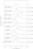 |
Fig. 1 Line profiles of the CH3OH emission observed in our sample. Profiles have been offset by υlsr (see Table 1) and normalized to unity with a factor indicated on the right part of the panel. |
The methanol emission is detected towards all sources at a signal-to-noise ratio of 15 or
more, with a peak Tmb varying from 0.6 to ~40 K (see
Fig. 1). For all sources, we detect wings or
multiple velocity components. Unlike CH3OH, the SO2 lines are
detected in 7 sources only and have a Gaussian shape. The HO line is seen toward 3 sources, W43-MM1, DR21(OH), and
IRAS 18089–1732; the line profiles exhibit a
Gaussian shape, except for DR21(OH) where the observed signal is more complex (see
Fig. 3 and following section). The HDO line
emission at 1 mm and 3 mm is detected toward 4 sources: W43-MM1, DR21(OH),
IRAS 18089 − 1732, and NGC 7538S. The HDO lines
are always either detected or both non-detected (see Fig. 2). We do not detect special features in the line profiles, except for DR21(OH)
whose line profile is most closely fitted by a two-component velocity model. Measured
parameters of single peaked lines are listed in Table 3. Methanol and other special features (such as the two velocity components in
DR21(OH)) are treated in Sect. 4.2. The 1.3 mm
spectrum of W43-MM1 shows detections of the expected transitions mixed up with additional
lines that we have identified (see Fig. 4). First,
emission line from HO is blended with an emission line of the
CH3OCH3 molecule at 203.408 GHz (see Table 4). We also detect a mixing between the SO2 transition and
emission at the frequency of 203.392 GHz (maybe C3H7CN, as
discovered by Belloche et al. 2009). This emission
seems to be real, as supported by its velocity width that is similar to other lines (see
Table 4). In the same spectrum, three other
emission lines from CH3OCH3 are clearly detected. All the lines have
a Gaussian shape. The 3 mm spectrum of W43-MM1 shows an unexpected feature near the
CH3OH line, coming from the NH2CHO molecule (see Table 4). One also notes in IRAS 18089 − 1732 and DR21(OH)
that the same group of CH3OCH3 lines seen in the W43-MM1 spectrum
are detected. One of them is blended with HO.
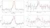 |
Fig. 2 Observations of the HDO (1–1) (top) and HDO (3–2) (bottom) emission lines from W43-MM1 (left) and NGC 7538S (right). For a clearer view, spectra have been smoothed by reducing the velocity resolution by a factor 2 (see Table 3 for the initial value). |
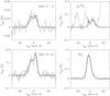 |
Fig. 3 Line profiles of the HDO at 3 mm (top left), 1 mm (bottom
left), H |
Characteristics of observed lines.
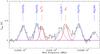 |
Fig. 4 Spectrum of H |
4.2. Line profiles
For all sources, except W43-MM1, the methanol emission line profiles exhibit wings (Fig. 1). Some of them are seen in both the blue and red-shifted parts (IRAS 05358 + 3543, IRAS 18151–1208 1, IRAS 18151–1208 2, NGC 7538S), and others only on one side (blue-shifted for IRAS 23385+6053, red-shifted for IRAS 18264–1152 and DR21(OH)S).
In addition to their wings, the methanol lines often show multiple velocity components. This is seen in IRAS 05358 + 3543, IRAS 18089 − 1732, IRAS 18151−1208-MM2, W43-MM1, and DR21(OH). The number of these components varies between 3 and 4 and their strength from ~1 to 40 K.
In DR21(OH), the 1.3 mm HDO transition exhibits a well defined two-component velocity
pattern. A double Gaussian fit reproduces the observed line with the parameters reported
in Table 5. The 3 mm HDO spectrum does not show the
two velocity peaks seen at 1.3 mm. A single velocity Gaussian profile provides a good fit
but only with a rather large ( > 10 km s-1) line width. We find that a more
convincing approach is to analyse this line with a two-line Gaussian model using fixed
velocities and widths derived from the 1.3 mm line, obtaining a good result. The fit
parameters are reported in Table 5. In the
HO spectrum, dimethyl ether and SO2 lines are
clearly detected. A close examination of all dimethyl ether lines reveals that not all
lines are well fitted with a single velocity component model because lines are too wide
compared to 1.3 mm HDO components. We choose to fit those lines with a two-component model
derived from the peak velocities observed in the methanol spectrum. We can then remove
from the spectrum the dimethyl ether contribution. The resulting spectrum shows a signal
well above the noise in the range expected for the HO transition. The higher velocity part is around the
2.9 km s-1 velocity observed in the 1.3 mm HDO spectrum and is well above the
noise. It is also well separated from the dimethyl ether line (no blending). On the other
hand, the lower velocity part, around the − 3.2 km s-1 component of the HDO
line is partly blended by dimethyl ether and the signal-to-noise ratio is lower. Fit
results are given in Table 5.
To estimate the HO emission line strength, and be consistent with the
observed HDO line profiles, the CH3OCH3 lines were first subtracted
from the spectrum using a model with two velocity components. The
CH3OCH3 and water emissions are expected to originate in the same
region because these two species are chemically linked. We then tentatively applied the
velocity component values to fit the HO emission. The resulting line emission parameters are
reported in Table 5, showing a blue-shifted
component that remains doubtful, even if it cannot be completely rejected (see Fig. 3). The SO2 line is detected but a single
velocity component fit does not provide a satisfying profile, where a two-velocity fit
constrained by the velocity difference (taken from the methanol velocities) gives a
slightly better result (see Table 5). The remaining
red wing on the SO2 line is mainly related to the dimethyl ether line. The
remaining blue signal on the foot of SO2 cannot be identified, but is weak
(70 mK).
Characteristics of the unexpected emission lines detected in W43-MM1.
Components in the line profile of DR21(OH).
5. Methanol maser emission
The CH3OH (J = 5−1,5 − 40,4E) transition is often detected as a so-called class I maser. Unlike class II masers, which originate in the immediate protostellar environment ( ≲ 103 AU), class I masers arise at some distance (≳104 AU) from the protostar. Here, shocks between jets and ambient gas cause local density and temperature enhancements where population inversions may occur (e.g. Minier et al. 2005). As a consequence, the maser emission lines are very sensitive to the local environment in which they appear and typically observed to have sharply peaked profile that can be distinguished from thermal, turbulent, or outflow emissions.
In our observations, the line profiles show that the maser and thermal emissions are mixed in different proportions. As we aim to trace shocks, we need to extract maser emission to ensure a reliably determination of any relation between the supposed evolutionary stages of our sources and the strengths of the shocks that may occur inside. An identical analysis is performed with profiles obtained by van der Tak et al. (2006) to extend our study.
5.1. Extraction method
To disentangle the thermal and maser contributions to the CH3OH line profiles, we use the extraction method of Caswell et al. (2000). The strong turbulence within these sources is also relevant a role too, leading to a larger width of the Gaussian line profile. This is why we enclose its effect under the term “thermal” used in this paper. We fit the MDC’s envelope contribution in each methanol profile by including the sources previously observed by van der Tak et al. (2006). The thermal emission is then fitted by a Gaussian component centred on the source velocity, an assumption motivated by all observations of class II or class I methanol masers (e.g. Caswell et al. 1995; Val’tts et al. 2000; Błaszkiewicz & Kus 2004) exhibiting maser line profiles that are sharply peaked and differ from a Gaussian shape. If the line becomes saturated, the maser profile is of course no longer narrow and the wings grow exponentially (Elitzur 1992) but this will never produce a “thermally-looking” profile. The possibility of blends of emission originating in multiple maser spots within the telescope beam is also real, and our assumption cannot be definitely verified until future interferometer observations are made.
Once the maser emission has been extracted, we measure its velocity-integrated area Amaser. We also compute the area Atherm of the thermal emission and derive the ratio Xm = Amaser/Atherm of these two quantities, to determine the sources in which the maser emission dominates.
5.2. Results
The results of the CH3OH class I maser emission extraction are given in Table 6, including results for the profiles observed by van der Tak et al. (2006).
The maser emission is dominant (Xm > 10) in two sources, IRAS 18151−1208-MM2 and DR21(OH). The very high emission intensity in these objects (Tpeak = 44.3 and 5.21 K, respectively), and the structure of their profiles (see Fig. 1) are consistent with this finding. A group of four sources (IRAS 05358 + 3543, IRAS 18089−1732, NGC 7538S, and IRAS 23385 + 6053) exhibit distinctive maser emission, (Xm ~ 1–2). A majority of objects exhibit weak maser emission (Xm ~ 0.1−1.0): IRAS 18151 − 1208-MM1, IRAS 18264 − 1152, W43-MM1, DR21(OH)-S, W33A, AFGL 2591, S140 IRS1, NGC 7538 IRS1, and NGC 7538 IRS9. In the three remaining objects, W3 IRS5, AFGL 2136, and AFGL 490, the maser emission seems to have disappeared and our measurements must be treated as upper limits (see Table 6).
Results of the CH3OH class I maser emission extraction.
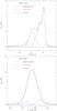 |
Fig. 5 Extraction of the methanol class I maser emission (blue line) from observations (black line) by fitting the thermal emission with a Gaussian profile at υlsr in two sources: DR21(OH) (top) and W43-MM1 (bottom). |
6. Molecular abundances
6.1. Modelling method
To derive molecular abundances from our observations, we use a global modelling process developed by van der Tak et al. (1999) and improved by Marseille et al. (2008). We first model the SED with the MC3D program (Wolf et al. 1999) to derive the mass and the temperature distributions inside the MDCs. The source model, i.e., its total luminosity, size, and density distribution is constrained by observations (see Tables 1 and 7), and uses dust properties derived by Draine & Lee (1984). We then transfer the density and temperature distribution to the RATRAN code (Hogerheijde & van der Tak 2000). This non-LTE radiative transfer code models the molecular line emissions observed, and thus we obtain the molecular abundances and the turbulence level, which are the two free parameters of this method.
The density distribution is characterized by a power law of the form
 (1)where n0 is the
density at the reference radius r0 (here 100 AU) obtained by a
fit to the optically thin emission of dust at millimetre wavelengths. The parameter
p is derived from continuum maps of MDCs or is set to be 1.5 according
to a quasi-static infall theory in the inner part of the object (Shu et al. 1987; Beuther et al.
2002c, see Table 7). The density and
temperature distributions are transferred to RATRAN when modelling the emission lines. The
best fit is obtained for a given gas turbulence velocity υT and a molecular
abundance relative to H2
(Xmol = nmol/nH2).
When an emission line is not detected, we derive an upper limit assuming a line velocity
width similar to the SO2 one (if available, otherwise we select the thermal
component of the methanol line) and refer to the abundance required for a
2σrms signal.
(1)where n0 is the
density at the reference radius r0 (here 100 AU) obtained by a
fit to the optically thin emission of dust at millimetre wavelengths. The parameter
p is derived from continuum maps of MDCs or is set to be 1.5 according
to a quasi-static infall theory in the inner part of the object (Shu et al. 1987; Beuther et al.
2002c, see Table 7). The density and
temperature distributions are transferred to RATRAN when modelling the emission lines. The
best fit is obtained for a given gas turbulence velocity υT and a molecular
abundance relative to H2
(Xmol = nmol/nH2).
When an emission line is not detected, we derive an upper limit assuming a line velocity
width similar to the SO2 one (if available, otherwise we select the thermal
component of the methanol line) and refer to the abundance required for a
2σrms signal.
Modelling parameters.
Modelling results.
6.2. Results
The HDO abundances obtained are between 10-13 and 10-9 when the line emission is detected (IRAS 18089−1732, W43-MM1, DR21(OH), and NGC 7538S; see Table 8). For other sources, the upper limits are between 10-13 and 10-11. IRAS 23385 + 6053 is an exception with the high upper limit of 1.5 × 10⁻⁹ for the HDO (31,2–22,1) transition. This high value (see Table 8) is mainly due to the compact shape of the source (0.05 pc compared with the size of the other sources, i.e. ~0.13 pc) that increases the beam dilution for high-excitation lines. Furthermore, IRAS 23385+6053 is a very dense and hot source (see Table 7) where a high abundance of water species is needed to reach the level of the critical density, permitting us to avoid strong self-absorption of the line emission (particularly for high-energy transitions), and explaining our high upper limit.
When the emission line of HO is detected (i.e. in IRAS 18089 − 1732, W43-MM1, and
DR21(OH)), its abundance is inferred to be between 10-11 and 10-9,
giving a  abundance estimation between 5 × 10⁻⁸ and
5 × 10⁻⁷, assuming a solar isotopic ratio
16O/18O = 500. Other sources give an upper limit between
10-13 and 10-12, hence a main water isotope abundance between
5 × 10-11 and 5 × 10⁻¹⁰. This result seems to indicate a low water
abundance in the MDC concerned, relative to the values measured by van der Tak et al. (2006, see
Tables 8 and 9), except for W43-MM1. The comparison of these abundances with those obtained
with the high-energy transition of HDO (Eup = 168 K, hence
close to the HO transition considered) show that they are consistent and
higher than the low-energy transition of HDO (Eup = 47 K),
except W43-MM1 (see Sect. 8 for a discussion of this result).
abundance estimation between 5 × 10⁻⁸ and
5 × 10⁻⁷, assuming a solar isotopic ratio
16O/18O = 500. Other sources give an upper limit between
10-13 and 10-12, hence a main water isotope abundance between
5 × 10-11 and 5 × 10⁻¹⁰. This result seems to indicate a low water
abundance in the MDC concerned, relative to the values measured by van der Tak et al. (2006, see
Tables 8 and 9), except for W43-MM1. The comparison of these abundances with those obtained
with the high-energy transition of HDO (Eup = 168 K, hence
close to the HO transition considered) show that they are consistent and
higher than the low-energy transition of HDO (Eup = 47 K),
except W43-MM1 (see Sect. 8 for a discussion of this result).
The HDO and HO abundances that we derive permit us to estimate the
HDO/H2O ratio in MDCs. Assuming that 16O/18O = 500, the
ratios are 33 × 10-4, 7 × 10⁻⁴, and 19 × 10-4 for
IRAS 18089−1732, W43-MM1, and DR21(OH), respectively. These values are obtained from
high-energy transition results (see Table 9). The
D/H ratio agrees with the values obtained by van der Tak
et al. (2006), giving values between 3 × 10⁻⁴ and
38 × 10-4. Our results and previous ones are reported in Table 9.
The CH3OH abundances are derived from the thermal emission components and are spread between 10-10 and 10-8, i.e. of the same order of magnitude as those derived by van der Tak et al. (2006) for mIRb MDCs. We note that W43-MM1 has the highest abundance in the sample, with a value reaching 5.4 × 10⁻⁷.
The modelling of the SO2 emission line implies an abundance of between 10-12 and 10-10 (see Table 8), which confirms previous estimations in MDCs (van der Tak et al. 2003; Wakelam et al. 2004). In particular, W43-MM1, IRAS 05358 + 3543, and IRAS 18264 − 1152 were already studied in Herpin et al. (2009), where a multi-transition evaluation of abundances is performed. For these sources, our results agree with their estimations. Even in IRAS 18264 − 1152, where an upper limit has been derived, our result is in accordance with the abundance estimated in their study.
We derive turbulent velocities higher than the speed of sound (υT = 0.85 − 2.9 km s-1 compared to as = 0.3 − 0.5 km s-1), confirming this MDC characteristic.
Abundance ratios.
A large number of sources in our sample are found to have a low upper limit to their
HO abundances (see Table 8). We suspect that most of the water is frozen in a solid state on the surface
on dust grains in these cases. As for HDO, IRAS 23385 + 6053 is an exception but this
result can be easily explained (see second paragraph). At the same time, some sources have
a clear water abundance enhancement: results on W43-MM1 confirm that it hosts a HMC
(already detected by Motte et al. 2003; Herpin et al. 2009), and others on IRAS 18089 − 1732
and DR21(OH) may indicate the same.
7. Correlations
To investigate how the molecular line emission is related to the physical properties of the MDCs, we compare the line fluxes and abundances to the mid-IR (12 m) emission seen by MSX and IRAS. Previous studies identified a link between mid-infrared emission and the physical evolution of MDCs (van der Tak et al. 2000a; Marseille et al. 2008). To increase the sample size, we include the data collected by van der Tak et al. (2006) for eight mIRb-MDCs.
7.1. Method
We compute the correlation factors ρx,y (see Appendix A) between the following parameters: mass M, luminosity L, thermal line width δυ (from the SO2 emission or, if not detected, thermal component of CH3OH), monochromatic luminosity L12 at 12 m, the molecular emission-line flux observed in CH3OH (masered Am, thermal At, the ratio Xm, and the abundance Xmol) and the abundance of H2O and HDO in sources where they are detected. Sources with upper limits to the 12 μm luminosity or the molecular emission-line flux are not used in the correlation analysis. Applying a two-tailed correlation test for N = 18 data points (or 7 for water), we reject correlation factors with values smaller than 0.49 (respectively 0.76) in absolute value. We also use the method of partial correlations (see Appendix A) to search for biases that could be introduced by the sample selection and extract the most probable real correlations, this allowing us to correct for false correlations induced by real ones (see Rodgers & Nicewander 1988, for a review of the subject).
7.2. Search for biases in the sample
In our systematic search for correlations, we first look for links between “standard variables” (mass, luminosity, and thermal line width and luminosities at 12 m). Apart from the thermal line widths, correlations are checked in logarithmic scales. To reliably compare our sources, we need to account for their different distances. To do so, we assume that they all are at a reference distance of 1.7 kpc by applying a correction factor to the flux densities, i.e. measuring monochromatic luminosities at 12 m and comparable methanol maser emissions. No correction is made for beam dilution, as the infrared and maser emissions are known to originate in a region much smaller than the beam size (point-like emission). We search for correlations with “standard variables” regardless of whether there is a physical reason to expect a correlation: this search acts as a reality check on our method.
Three relations are identified when applying the correlation method. First, a link seems to exist between the mass and the luminosity of the sources (ρM,L = 0.50, thus 97.5% of a chance of being real statistically). However, a partial correlation analysis rejects this trend by giving a value under the confidence threshold (ρML,Δυ = 0.36) when keeping Δυ constant. Second, a weak correlation may exist between thermal line velocity widths and the luminosity of the sources (ρΔυ,L = 0.49) but again partial correlation factors reduce this value to 0.34, by keeping the mass constant. This result has a 16.6% probability of being obtained by chance, which is too high to claim that a link exists. A third correlation appears between luminosity and mid-IR emission, with ρL,L12 = 0.80. This trend is clearly confirmed by partial correlation factors, indicating that we can be confident in this result to a level of more than 99.9% (see Fig. 6).
7.3. Methanol correlations
We show in Sect. 5 that two components can be extracted from the methanol line emission: a thermal (At) and a maser one (Am). As these two components reflect two different characteristics of the sources, we try to find correlations between them and the intrinsic variables (mass, luminosity, etc.). We also test a possible correlation with the ratio Xm and the abundance Xmol. The overall correlation matrix, summarizing the results, is given in Table 10.
Correlation matrix for the sample and the CH3OH emission analysis.
The first correlation relates the mid-IR luminosities to the maser component (ρAm,L12 = −0.67). The correlation factor is negative, indicating an anti-correlation between these two variables (see Fig. 6). This trend is confirmed by the partial correlation analysis, reducing the correlation factor to − 0.65 when the thermal component is assumed to be constant, and giving approximately a 98.5% of chance of this correlation being real. We note that there is no significant correlation of the integrated (thermal + maser) CH3OH line flux in our data. A partial correlation analysis demonstrates that the weakening of the CH3OH maser flux with increasing 12 μm luminosity is not caused by increasing distance.
In addition, we find two correlations associated with At. The first one indicates that thermal CH3OH emission increases with the mass of the object (ρAt,M = 0.70, see Fig. 6). The partial correlation analysis confirms this trend and, at its most extreme, decreases the correlation factor to 0.65 when L is assumed to be constant. There is a probability of lower than 0.4% that this trend is obtained by chance. The thermal emission is also linked to the maser emission, the correlation factor being equal to 0.76 (see Fig. 6). The study of partial correlation factors slightly decreases the initial value to 0.75, giving a high chance (99.9% statistically) for this result being real.
Three other links, all related to the ratio Xm (see Table 10), are found but rejected by the partial correlation analysis, except the correlation with the maser emission which increases (up to 0.96; this result is obvious as Xm = Am/At). More precisely, partial correlation factors obtained for other correlations are well below the threshold, with |ρ| = 0.27 at the maximum, hence there is more than a 27% chance of obtaining this result by luck. Thus, this ratio is interesting but a bit less relevant than Am.
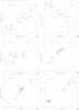 |
Fig. 6 Correlation plots between a) monochromatic luminosities at 12 m and
source luminosity; b) monochromatic luminosities at 12 m and maser
component of CH3OH emission line; c) masses of HMPOs and the
thermal component of CH3OH emission lines; d) the thermal
and the maser component of CH3OH emission lines; e) the
maser-to-thermal emission ratio and the maser emission; f) the
molecular abundances of HDO and H |
Correlation matrix for the water emission analysis.
7.4. Water correlations
We now consider the water abundances, including numbers obtained in other MDCs (van der Tak et al. 2006). We also search for possible correlations with the deuteration level D/H. Only the sources where water line emission is detected are included, hence 8 MDCs. As a consequence, the confidence threshold for a real correlation is now 0.756, assuming a two-tailed test (or two-σ test).
First of all, the analysis of biases in this restricted sample reveals, again, a link between the mid-IR luminosity at 12 m L12 and the total luminosity L (see Table 11). Partial correlation factors confirm this trend with a final correlation factor of 0.79, hence 98% of chance of this relation being real. This is a strong indication that these two variables are correlated, even when a smaller sample of sources is chosen.
Another correlation is found, between the mid-IR emission L12
and the HDO abundance
(ρL12,HDO = 0.80, see Table 11). This is not confirmed by the partial correlation
analysis, for which we measure a factor beneath the threshold when the
HO abundance is assumed to be constant at
 , hence a 12.9% chance of having obtained this result with
luck, statistically.
, hence a 12.9% chance of having obtained this result with
luck, statistically.
The last connection that we find is between the HDO and HO ( , see Table 11 and
Fig. 6). This relation is strong and the partial
correlation method confirms this trend by decreasing, at most, the correlation factor to
0.90 when the mid-IR flux density L12 is assumed to be
constant. This value indicates that our result is real in more than 99.8% of the cases.
This correlation was already noted by eye (Table 8)
and confirms that the D/H ratio is of the same order of magnitude in all studied MDCs.
, see Table 11 and
Fig. 6). This relation is strong and the partial
correlation method confirms this trend by decreasing, at most, the correlation factor to
0.90 when the mid-IR flux density L12 is assumed to be
constant. This value indicates that our result is real in more than 99.8% of the cases.
This correlation was already noted by eye (Table 8)
and confirms that the D/H ratio is of the same order of magnitude in all studied MDCs.
More globally, our study illustrates that water abundance (hence detection) does not depend on a basic characteristic of HMPOs (such as their mass or luminosity) but needs further investigations in each specific source. This point is discussed in Sect. 8.2.
8. Discussion
8.1. Methanol masers: shocks in embedded objects?
Our study reveals a clear link between the mid-IR brightness of the 18 MDCs (including the sample by van der Tak et al. 2006) that we have observed and the methanol maser emission at 84.5 GHz (class I maser). Unlike class II masers, which originate in static regions near massive protostars, class I masers are known to occur in extended zones, at some distance from the star formation sites (~104 AU), where molecular outflows interact with the surrounding medium (Minier et al. 2005). Cyganowski et al. (2009) study 20 massive young stellar objects observed with interferometry to confirm this behaviour, and claim that methanol class I masers trace the molecular outflows around them.
Molecular outflows are indicators of an accretion process, and are known to decrease in intensity with time as the protostar evolves (low-mass case, see Bontemps et al. 1996). Presenting an early stage of massive star formation, most of MDCs harbour powerful outflows. However, extraction of molecular outflow strength is biased by the unknown orientation and the possible source multiplicity, and no clear drop in strength can be observed between mIRq- and mIRb-MDCs (Beuther et al. 2002a; Marseille et al. 2008). Furthermore, the decrease in power is suspected to occur at a later stage, i.e. in MDCs where an HII region has developed. As a consequence, the variation in the methanol class I maser emission cannot be linked to a drop in the molecular outflow strength from mIRq to mIRb sources. Like class II masers, class I maser emission needs a very specific environment, with a sufficient spatial extend. Moreover, the detection of multiple velocity components implies that the class I maser sites are localized at the interface between the molecular outflows and the ambient gas. We can assume that mIRq sources contain more favourable zones where this kind of maser emission is more likely to occur.
The origin of the varying mid-IR brightnesses in MDCs remains quite unclear. On the one hand, modelling their spectral energy distribution shows that the mid-IR emission is critically dependent on the line of sight when molecular outflows dig a cavity from which IR emission can escape (Robitaille et al. 2006; van der Tak et al. 2006; Marseille et al. 2008). Thus the variations in mid-IR brightness are orientation-dependent and do not reflect any difference in evolutionary stage. On the other hand, chemical models and observations of sulphur-bearing molecules or cold gas tracers such as N2H+ seem to indicate that mid-IR brighter sources are more evolved and warmer, relative to more quiet ones (Reid & Matthews 2008; Marseille et al. 2008; Herpin et al. 2009).
The anti-correlation that we find between the 12 m luminosity and the maser emission makes the situation clearer. Indeed, the hypothesis that the variations in mid-IR brightness are due to orientation differences cannot explain this trend, as the maser emission is not affected by the line of sight direction. Furthermore, the multiple velocity components would be more easily detected if the molecular outflows, i.e. the cavity from where the mid-IR is emitted, were to follow the line of sight (case of mIRb-MDCs). However, we observe the opposite trend. A valid interpretation defines mIRq-HMPOs as embedded objects, in which the envelope mainly interacts with outflows. Here, the term “embedded” must be defined to avoid confusion. Our study has found that the envelope masses of MDCs are not linked to their mid-IR brightness, hence are not sufficient to determine wether they are embedded or not. Taking into account the material distribution, the SED modelling of MDCs shows that their spherically symmetric distribution is responsible for their mid-IR emission from MDCs (Robitaille et al. 2006; Marseille et al. 2008). In this sense, our study shows that mIRq-MDCs are embedded sources. Bright mid-IR objects may thus have more flattened envelopes than weak mid-IR ones. From an observational point of view, this idea is supported by the Kurtz et al. (2004) study of the IRAS 23385 + 6053 source where maser emission is detected around the source velocity (at −49.7 km s-1 and −51.7 km s-1). The conclusion of this study is that this observation can be explained by accretion shocks near the central object. This could explain also what we observe for W43-MM1, where strong clues of infall toward this source have been detected (Herpin et al. 2009).
Nevertheless, an embedded phase does not imply that they correspond to an earlier stage of evolution. For example, this characteristic can be a direct consequence of the initial conditions of the MDC formation. However, our results support a scenario in which the initial collapsing clump, radially concentrated, is disrupted by the molecular bipolar outflows during the accretion phase. Moreover, the mid-IR brightness and evolutionary stage of MDCs are linked.
8.2. The origin of water emission
Previous results on HDO and HO detections in mIRb-MDCs obtained by van der Tak et al. (2006) demonstrated that these objects are not
systematically strong H2O emitters. Our study has a similar detection rate
(just below ~50%) and does not show any evidence of an emission enhancement from
mIRq to mIRb sources. This contradicts the hypothesis that warmer objects should be
stronger emitters. Indeed, a warmer environment should increase the release of water in
the gas phase from the ice on dust grains. Thus, the origin of the strong line emission of
water species in particular sources cannot be linked to the “quiet” versus “bright”
scheme. Each source must be treated individually.
The IRAS 18089–1732 MDC is the most luminous object in the mIRq sample
(3.2 × 10⁴ L⊙), and is also the source where the
turbulence level is the highest (υT = 1.2 − 2.6 km s-1). The
discernible methanol class I maser emission in this object
(Xm = 1.42) is indicative of interactions between the
molecular outflows and the envelope. We have shown that the abundance of H2O
and HDO is high enough to be detected (see Table 8). We thus conlude that, in IRAS 18264 − 1152, the water abundance enhancement is
caused by the large amount of energy available from luminosity, gas turbulence, and
molecular outflows (shocks). In addition, the detection of unexpected dimethyl-ether
emission in the HO spectrum suggests that complex chemical components are
released in the gas phase, including the water ice. We propose that the enhancement
originates in a hot molecular core whose presence may also explain why water is detected
in this source.
In W43-MM1, many molecular rotational transitions have been detected, covering a wide range of energy (Herpin et al. 2009). The large amount of detected species, even unexpected complex molecules, are indicative of an extended hot molecular core, and make this source of particular interest. Moreover, this region is suspected to be in global infall (Motte et al. 2003; Herpin et al. 2009). This very likely explains the very high abundances (see Table 9) in this source: the ice on dust grains must have evaporated, increasing the water abundance to 2 × 10⁻⁶.
Water line profiles towards DR21(OH) exhibit a double velocity component that may be
linked to powerful bipolar outflows, the water emission being produced by shocks between
molecular outflows and the massive envelope. This is confirmed by the strong methanol
class I maser emission (Xm = 1.58), and wherein three
components are identified, but the velocity components observed in H2O and HDO
profiles differ from the velocity components of the maser emission (see Table 5). In addition, this scenario (increase in the amount
of water species in the gas phase due to shocks) should apply to IRAS 18151 − 1208-MM2,
the most powerful methanol maser emitter (Xm = 13.9), but no
HDO and HO emission is detected. Hence, we conclude that shocks in
DR21(OH) are not the origin of the abundance enhancement of water. DR21(OH) is one of
three sources where unexpected detections of dimethyl-ether have been observed, showing
that a hot molecular core takes place there. This is the best argument to explain the
water abundance in this source.
On the other hand, HDO is detected in the source NGC 7538S, where there is no indication
of a hot core. Furthermore, this object is not a strong methanol class I maser emitter
(Xm = 0.21), showing that no strong shocks occur inside it.
The origin of the water detection is then more difficult to explain. In addition, our
modelling of NGC 7538S shows that the water abundance is not particularly high compared to
upper limits derived for other sources (see Table 8), even if this MDC has the highest temperature of the sample, well above the
others (⟨T⟩ = 38.7 K). This high temperature is caused by the small size
of this source (0.05 pc) combined with its high luminosity
(1.3 × 10⁴ L⊙). Therefore, we suppose that the
emission of water species in NGC 7538S, while not as abundant as those in hot cores, is
stronger due to this high temperature. However, the derived abundances are consistent with
an abundance jump of 1 × 10⁴ in the hottest part of NGC 7538S. Indeed, we
obtained low but almost equivalent values when considering either low or high energy level
transitions (~1 × 10-13). Another possibility would be that NGC 7538S
harbors a brand new hot core. In that case, primal ices forming on dust grains in the
atomic phase of diffuse clouds are strongly deuterated by the formation mechanism (Lipshtat et al. 2004; Cazaux et al. 2008). This could explain why HDO is detected while
HO is not, these primal ices being first desorbed when a hot
core starts to develop.
Our study of a large sample of MDCs permits us to conclude that the water detection in these objects is not linked to their mid-IR brightness, i.e. a different evolutionary stage or a different distribution of materials. In addition, it shows that water detection is associated with a hot molecular core. This seems reasonable as in the gas phase hot cores are known to release complex molecules that are detected, while ice on dust grains evaporates. In rare cases, such as NGC 7538S, water line emission may be detected due to a globally high temperature in the source.
8.3. mIRq vs mIRb: review of common and different properties
Several clues show that mIRq- and mIRb-MDCs have similar properties. First, previous work on large samples of MDCs indicate that the velocity widths of emission lines are dominated by gas turbulence (υT = 0.8 − 2.9 km s-1), whose corresponding width is much higher than the thermal width (Beuther et al. 2002b; Motte et al. 2007). Our observations confirm this result, and that this high turbulence may be the consequence of the initial cloud collapse, as suspected in large-scale filaments (e.g. DR21 in Cygnus X, see Motte et al. 2007; or the Ophiuchus main cloud, see André et al. 2007). In this context, the turbulence is supposed to dissipate by means of ambipolar diffusion while the MDC evolves, leading to a quasi-static collapse (see Ward-Thompson et al. 2007, for a review). Our study shows that the turbulence does not vary between mIRq- and mIRb-MDCs, indicating that their evolutionary stages are similar. We also note that the range of masses in our sample (200 − 2000 M⊙) has no impact on the mid-IR brightness of the sources. To first order, the most massive sources should have a higher opacity at mid-IR wavelengths. Our study contradicts this simple view. The emission process of mid-IR is complex in MDCs, and must include other parameters. Previous work on the SED modelling of MDCs show that the density distribution plays a major role in this issue (Robitaille et al. 2006; Marseille et al. 2008).
Our work has revealed that the water abundance in MDCs is independent of their mid-IR brightness. The detection ratio in mIRq and mIRb sources is the same (slightly below 50%). Water abundances derived are similar, with a wide range of values in the external cold parts of the objects (between ~1 × 10-13 and ~1 × 10⁻⁹). From our study, we conclude that most objects for which water species are detected contain a more or less extended hot molecular core. Finally, we have found that mIRq and mIRb sources share the same deuteration ratio D/H ~ (5–40) × 10-4. As already reported in van der Tak et al. (2006), this value is one hundred times higher than the interstellar ratio, and confirms that the molecular emission observed is coming from evaporated ices.
These results illustrate the difficulty in differentiating between the mIRq and mIRb classes. The origin of this distinction is linked to the class 0 and class I definitions for low-mass protostars (André et al. 1993), where the mid-IR luminosity is compared to the overall luminosity of the sources. A ratio Lλ < 25 μm/Lbol < 0.3% indicates a class 0 object, and a class I object in the opposite case. This definition was extended to MDCs where a similar behaviour at mid-IR wavelengths was observed, and “quiet” sources were suspected to represent an earlier stage of the massive star formation evolution. However, it appears more and more clearly that directly applying definitions from low-mass protostars to high-mass star-forming regions is unwise and may not be adapted to correctly transcribe different evolutionary stages. This is caused by the multiplicity of MDCs, that are now identified as massive proto-clusters, but also to the presence of powerful outflows, hot molecular cores and suspected infall (Motte et al. 2003; van der Tak et al. 2006; Leurini et al. 2007b; Ward-Thompson et al. 2007; Marseille et al. 2008; Herpin et al. 2009). Furthermore, we show that the observed variation in mid-IR brightness seems to be associated with the matter distribution around the protocluster, being more or less spherically symmetric.
Interpreting mIRq sources as more embedded objects supports the idea that they represent an earlier stage of the massive star formation. Indeed, with the hypothesis that MDCs start in a deeply embedded phase where matter is then flattened by powerful outflows, as the methanol class I maser trend seems to illustrate, the evolutionary sequence from mIRq- to mIRb-MDCs is still valid.
9. Conclusions
We summarize the main conclusions of our study:
-
1.
Using a correlation method, we have derived a link between themethanol class I maser emission and the mid-IR luminosity of theMDCs that we observed. We propose that this link can beexplained by the mIRq sources being more deeply embedded, i.e.having a more spherically symmetric distribution of theirenvelope material, creating a favourable environment for thecreation of these masers.
-
The detection of line emission from H2O and HDO is linked to a hot molecular core, independent of the mid-IR brightness.
-
2.
The study of the overall sample has demonstrated that MDCs have many common properties: their size (0.1 pc), mass (~200−2000 M⊙), luminosity (~1 × 10⁴ L⊙), turbulent velocity of the gas (υT = 1−3 km s-1), incidence of hot cores ( ≲ 50%), and deuteration level (D/H ~ 5−40 × 10-4). This implies the idea that these objects can be treated as a single class, and that they constitute a cluster of protostars, some of them being massive.
-
3.
The classification of MDCs is complex due to their multiplicity and the multiple physical processes (independent of their evolutionary stage) that occur inside, which have a strong impact on observations, i.e. hot molecular core presence, and powerful outflows, suspected collapse. We finally suggest that the mid-IR “quiet” and “bright” classification needs more investigation but is still relevant when we assume that mIRq sources represent an earlier stage of massive star formation than mIRb ones.
In the near future, further investigation of the mIRq versus mIRb-MDCs evolutionary stage problem will be possible, particularly by means of direct water line detections with the Herschel-HIFI instrument and the high-angular resolution of present (IRAM, SMA, CARMA) and future (ALMA) interferometers. These may provide us with the final arguments permitting us to find a coherent classification, by age, of the MDCs, hence allowing us to describe a complete evolution scenario leading to the formation of massive stars.
Acknowledgments
We thank the editor, Malcolm Walmsley, for many comments that improved the quality of the manuscript.
References
- André, P., Ward-Thompson, D., & Barsony, M. 1993, ApJ, 406, 122 [NASA ADS] [CrossRef] [Google Scholar]
- André, P., Belloche, A., Motte, F., & Peretto, N. 2007, A&A, 472, 519 [NASA ADS] [CrossRef] [EDP Sciences] [Google Scholar]
- Barvainis, R., & Deguchi, S. 1989, AJ, 97, 1089 [NASA ADS] [CrossRef] [Google Scholar]
- Belloche, A., Garrod, R. T., Müller, H. S. P., et al. 2009, A&A, 499, 215 [NASA ADS] [CrossRef] [EDP Sciences] [Google Scholar]
- Beuther, H., Schilke, P., Gueth, F., et al. 2002a, A&A, 387, 931 [NASA ADS] [CrossRef] [EDP Sciences] [Google Scholar]
- Beuther, H., Schilke, P., Menten, K. M., et al. 2002b, ApJ, 566, 945 [NASA ADS] [CrossRef] [Google Scholar]
- Beuther, H., Schilke, P., Sridharan, T. K., et al. 2002c, A&A, 383, 892 [NASA ADS] [CrossRef] [EDP Sciences] [Google Scholar]
- Beuther, H., Walsh, A., Schilke, P., et al. 2002d, A&A, 390, 289 [NASA ADS] [CrossRef] [EDP Sciences] [Google Scholar]
- Błaszkiewicz, L., & Kus, A. J. 2004, A&A, 413, 233 [NASA ADS] [CrossRef] [EDP Sciences] [Google Scholar]
- Bonnell, I. A., Bate, M. R., Clarke, C. J., & Pringle, J. E. 1997, MNRAS, 285, 201 [NASA ADS] [CrossRef] [Google Scholar]
- Bonnell, I. A., Bate, M. R., Clarke, C. J., & Pringle, J. E. 2001, MNRAS, 323, 785 [NASA ADS] [CrossRef] [Google Scholar]
- Bonnell, I. A., Bate, M. R., & Zinnecker, H. 1998, MNRAS, 298, 93 [NASA ADS] [CrossRef] [Google Scholar]
- Bontemps, S., Andre, P., Terebey, S., & Cabrit, S. 1996, A&A, 311, 858 [NASA ADS] [Google Scholar]
- Bontemps, S., Motte, F., Csengeri, T., & Schneider, N. 2010, A&A [0909.2315] [Google Scholar]
- Boonman, A. M. S., Doty, S. D., van Dishoeck, E. F., et al. 2003, A&A, 406, 937 [NASA ADS] [CrossRef] [EDP Sciences] [Google Scholar]
- Caswell, J. L., Vaile, R. A., Ellingsen, S. P., & Norris, R. P. 1995, MNRAS, 274, 1126 [NASA ADS] [Google Scholar]
- Caswell, J. L., Yi, J., Booth, R. S., & Cragg, D. M. 2000, MNRAS, 313, 599 [NASA ADS] [CrossRef] [Google Scholar]
- Cazaux, S., Caselli, P., Cobut, V., & Le Bourlot, J. 2008, A&A, 483, 495 [NASA ADS] [CrossRef] [EDP Sciences] [Google Scholar]
- Cernicharo, J., Thum, C., Hein, H., et al. 1990, A&A, 231, L15 [NASA ADS] [Google Scholar]
- Cyganowski, C. J., Brogan, C. L., Hunter, T. R., & Churchwell, E. 2009, ApJ, 702, 1615 [NASA ADS] [CrossRef] [Google Scholar]
- Draine, B. T., & Lee, H. M. 1984, ApJ, 285, 89 [Google Scholar]
- Edris, K. A., Fuller, G. A., & Cohen, R. J. 2007, A&A, 465, 865 [NASA ADS] [CrossRef] [EDP Sciences] [Google Scholar]
- Elitzur, M. 1992, Astronomical masers Astrophysics and Space Science Library, 170 [Google Scholar]
- Girart, J. M., Beltrán, M. T., Zhang, Q., Rao, R., & Estalella, R. 2009, Science, 324, 1408 [NASA ADS] [CrossRef] [PubMed] [Google Scholar]
- Guilloteau, S., & Lucas, R. 2000, in Imaging at Radio through Submillimeter Wavelengths, ed. J. G. Mangum, & S. J. E. Radford, ASP Conf. Ser., 217, 299 [Google Scholar]
- Harwit, M., Neufeld, D. A., Melnick, G. J., & Kaufman, M. J. 1998, ApJ, 497, L105+ [NASA ADS] [CrossRef] [Google Scholar]
- Haschick, A. D., Baan, W. A., & Menten, K. M. 1989, ApJ, 346, 330 [NASA ADS] [CrossRef] [Google Scholar]
- Henriksen, R., Andre, P., & Bontemps, S. 1997, A&A, 323, 549 [NASA ADS] [Google Scholar]
- Herpin, F., Marseille, M., Wakelam, V., Bontemps, S., & Lis, D. C. 2009, A&A, 504, 853 [NASA ADS] [CrossRef] [EDP Sciences] [Google Scholar]
- Hogerheijde, M. R., & van der Tak, F. F. S. 2000, A&A, 362, 697 [NASA ADS] [Google Scholar]
- Kurtz, S., Hofner, P., & Álvarez, C. V. 2004, ApJS, 155, 149 [NASA ADS] [CrossRef] [Google Scholar]
- Leurini, S., Beuther, H., Schilke, P., et al. 2007a, A&A, 475, 925 [NASA ADS] [CrossRef] [EDP Sciences] [Google Scholar]
- Leurini, S., Beuther, H., Schilke, P., et al. 2007b, A&A, 475, 925 [NASA ADS] [CrossRef] [EDP Sciences] [Google Scholar]
- Lipshtat, A., Biham, O., & Herbst, E. 2004, MNRAS, 348, 1055 [NASA ADS] [CrossRef] [Google Scholar]
- Marseille, M., Bontemps, S., Herpin, F., van der Tak, F. F. S., & Purcell, C. R. 2008, A&A, 488, 579 [NASA ADS] [CrossRef] [EDP Sciences] [Google Scholar]
- McKee, C. F., & Tan, J. C. 2003, ApJ, 585, 850 [NASA ADS] [CrossRef] [MathSciNet] [Google Scholar]
- Minier, V., Burton, M. G., Hill, T., et al. 2005, A&A, 429, 945 [NASA ADS] [CrossRef] [EDP Sciences] [Google Scholar]
- Molinari, S., Brand, J., Cesaroni, R., & Palla, F. 1996, A&A, 308, 573 [NASA ADS] [Google Scholar]
- Molinari, S., Testi, L., Brand, J., Cesaroni, R., & Palla, F. 1998, ApJ, 505, L39 [NASA ADS] [CrossRef] [Google Scholar]
- Molinari, S., Faustini, F., Testi, L., et al. 2008, A&A, 487, 1119 [NASA ADS] [CrossRef] [EDP Sciences] [Google Scholar]
- Motte, F., Schilke, P., & Lis, D. C. 2003, ApJ, 582, 277 [NASA ADS] [CrossRef] [Google Scholar]
- Motte, F., Bontemps, S., Schilke, P., et al. 2007, A&A, 476, 1243 [NASA ADS] [CrossRef] [EDP Sciences] [Google Scholar]
- Reid, M. A., & Matthews, B. C. 2008, ApJ, 675, 1343 [NASA ADS] [CrossRef] [Google Scholar]
- Robitaille, T. P., Whitney, B. A., Indebetouw, R., Wood, K., & Denzmore, P. 2006, ApJS, 167, 256 [NASA ADS] [CrossRef] [Google Scholar]
- Rodgers, J. L., & Nicewander, W. A. 1988, The American Statistician, 42, 59 [Google Scholar]
- Sandell, G., Wright, M., & Forster, J. R. 2003, ApJ, 590, L45 [NASA ADS] [CrossRef] [Google Scholar]
- Shu, F. H., Adams, F. C., & Lizano, S. 1987, ARA&A, 25, 23 [Google Scholar]
- Shu, F., Najita, J., Galli, D., Ostriker, E., & Lizano, S. 1993, in Protostars and Planets III, ed. E. H. Levy, & J. I. Lunine, 3 [Google Scholar]
- Sridharan, T. K., Beuther, H., Schilke, P., Menten, K. M., & Wyrowski, F. 2002, ApJ, 566, 931 [NASA ADS] [CrossRef] [Google Scholar]
- Szymczak, M., Kus, A. J., & Hrynek, G. 2000, MNRAS, 312, 211 [NASA ADS] [CrossRef] [Google Scholar]
- Val’tts, I. E., Ellingsen, S. P., Slysh, V. I., et al. 2000, MNRAS, 317, 315 [NASA ADS] [CrossRef] [Google Scholar]
- van der Tak, F. F. S., van Dishoeck, E. F., Evans, I. N. J., Bakker, E. J., & Blake, G. A. 1999, ApJ, 522, 991 [NASA ADS] [CrossRef] [Google Scholar]
- van der Tak, F. F. S., van Dishoeck, E. F., Evans, I. N. J., & Blake, G. A. 2000a, ApJ, 537, 283 [NASA ADS] [CrossRef] [Google Scholar]
- Van der Tak, F. F. S., van Dishoeck, E. F., & Caselli, P. 2000b, A&A, 361, 327 [NASA ADS] [Google Scholar]
- van der Tak, F. F. S., Boonman, A. M. S., Braakman, R., & van Dishoeck, E. F. 2003, A&A, 412, 133 [NASA ADS] [CrossRef] [EDP Sciences] [Google Scholar]
- van der Tak, F. F. S., Walmsley, C. M., Herpin, F., & Ceccarelli, C. 2006, A&A, 447, 1011 [NASA ADS] [CrossRef] [EDP Sciences] [Google Scholar]
- van Dishoeck, E. F., & Helmich, F. P. 1996, A&A, 315, L177 [NASA ADS] [Google Scholar]
- Wakelam, V., Castets, A., Ceccarelli, C., et al. 2004, A&A, 413, 609 [NASA ADS] [CrossRef] [EDP Sciences] [Google Scholar]
- Ward-Thompson, D., André, P., Crutcher, R., et al. 2007, in Protostars and Planets V, ed. B. Reipurth, D. Jewitt, & K. Keil, 33 [Google Scholar]
- Wolf, S., Henning, T., & Stecklum, B. 1999, A&A, 349, 839 [NASA ADS] [Google Scholar]
- Yorke, H. W., & Sonnhalter, C. 2002, ApJ, 569, 846 [NASA ADS] [CrossRef] [Google Scholar]
- Zapata, L. A., Rodríguez, L. F., Ho, P. T. P., Beuther, H., & Zhang, Q. 2006, AJ, 131, 939 [NASA ADS] [CrossRef] [Google Scholar]
- Zinnecker, H., & Yorke, H. W. 2007, ARA&A, 45, 481 [NASA ADS] [CrossRef] [Google Scholar]
Appendix A: Elements of correlation theory
For more detail and a global review of correlation factor usage, we refer to Rodgers & Nicewander (1988).
A.1. Correlation factor definition
Given two variables x and y with N
elements xi and
yi, the correlation factor
ρx,y between these two variables is
measured to be 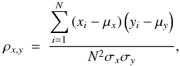 (A.1)where
 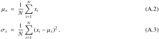 A correlation factor has a value between
− 1 and 1, a positive value indicating a correlation between the two variables and a
negative value indicating an anti-correlation. If two variables are distributed randomly
following a normal law, the density of probability
P(ρ) of finding a correlation factor between
ρ and ρ + dρ is given by
A correlation factor has a value between
− 1 and 1, a positive value indicating a correlation between the two variables and a
negative value indicating an anti-correlation. If two variables are distributed randomly
following a normal law, the density of probability
P(ρ) of finding a correlation factor between
ρ and ρ + dρ is given by
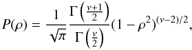 (A.4)where Γ is the classic gamma function, and
ν = N − 2 where N is the number of
elements (see Fig. A.1 for plots at different
N). Thus, the absolute value of the correlation gives, as a function
of the number of elements N, a percentage of the distribution
(xi,yi)
obtained by chance. The higher the absolute value of the correlation factor is, the
lower this percentage. As an example, a correlation factor of − 0.5 obtained with 20
elements has a good chance (97.5%) of being real. With only 6 elements, the same
correlation factor has a lesser chance (68.8%) of being real.
(A.4)where Γ is the classic gamma function, and
ν = N − 2 where N is the number of
elements (see Fig. A.1 for plots at different
N). Thus, the absolute value of the correlation gives, as a function
of the number of elements N, a percentage of the distribution
(xi,yi)
obtained by chance. The higher the absolute value of the correlation factor is, the
lower this percentage. As an example, a correlation factor of − 0.5 obtained with 20
elements has a good chance (97.5%) of being real. With only 6 elements, the same
correlation factor has a lesser chance (68.8%) of being real.
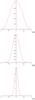 |
Fig. A.1 Plots of the P(ρ) with different number of elements on the sample studied: a) with N = 10, b) with N = 25, and c) with N = 100. |
One can note that the P(ρ) function peaks more and
more around ρ = 0 while N increases. More precisely,
the standard deviation of the P(ρ) distribution is
given by 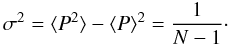 (A.5)It is then common practise to perform a
two-tailed (two-sigma) test to reject the null-hypothesis, i.e. that the
(xi,yi)
points does not follow a distribution of two random variables. This permits us to define
a correlation factor threshold ρt equal to
2σ to claim wether a correlation has a good chance of being real or
not
(A.5)It is then common practise to perform a
two-tailed (two-sigma) test to reject the null-hypothesis, i.e. that the
(xi,yi)
points does not follow a distribution of two random variables. This permits us to define
a correlation factor threshold ρt equal to
2σ to claim wether a correlation has a good chance of being real or
not 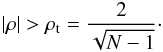 (A.6)This formula justifies that
N ≥ 6, which is a necessary criterion to obtain a threshold lower
than 1. In the case of our study, we used the two-sigma test to discriminate between
true and false correlation.
(A.6)This formula justifies that
N ≥ 6, which is a necessary criterion to obtain a threshold lower
than 1. In the case of our study, we used the two-sigma test to discriminate between
true and false correlation.
A.2. Partial correlations
When studying multiple variables at the same time, it is very often useful to have a clear view of the links between the variables, and first determine wether they exist or not. Existence of these links can be identified by determining the correlation factors of pairs of variables (see section above).
Unfortunately, the use of correlation factors restricts the study to pairs of variables, which can lead to the identification of false links, i.e. two variables that seems to be correlated when a third variable is the true origin of this link. One can take the example of a sample of pupils of all ages. A raw study of correlations between their ages, weights, and scientific levels will certainly make establish a false link: between the weight and the scientific level. Indeed, we can easily understand that their ages are at the origin of their growth, physically and intellectually. For a sample in which this logical deductions would be impossible, how can we distinguish true from false correlations?
The use of partial correlations permits us to avoid this issue. Giving a set of three
variables x, y, and z, partial
correlation ρxy,z derives the correlation
factor between two variables (for example x and y),
assuming that the third one z remains constant during the measurements.
The partial correlation factor is then given by
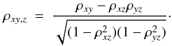 (A.7)If the partial correlation factor obtained
is below the confidence threshold chosen or has a different sign from the standard
correlation factor, then the link between the two variables is false.
(A.7)If the partial correlation factor obtained
is below the confidence threshold chosen or has a different sign from the standard
correlation factor, then the link between the two variables is false.
For a large set of variables {Xi}, all the links obtained by standard correlations factors ρXi,Xj must be verified with a systematic checking of all partial correlations associated with it, i.e. all ρXiXj,Xk ≠ { i,j } must be above the threshold of confidence and have the same sign as ρXi,Xj.
All Tables
All Figures
|
Fig. 1 Line profiles of the CH3OH emission observed in our sample. Profiles have been offset by υlsr (see Table 1) and normalized to unity with a factor indicated on the right part of the panel. |
| In the text | |
|
Fig. 2 Observations of the HDO (1–1) (top) and HDO (3–2) (bottom) emission lines from W43-MM1 (left) and NGC 7538S (right). For a clearer view, spectra have been smoothed by reducing the velocity resolution by a factor 2 (see Table 3 for the initial value). |
| In the text | |
|
Fig. 3 Line profiles of the HDO at 3 mm (top left), 1 mm (bottom
left), H |
| In the text | |
|
Fig. 4 Spectrum of H |
| In the text | |
|
Fig. 5 Extraction of the methanol class I maser emission (blue line) from observations (black line) by fitting the thermal emission with a Gaussian profile at υlsr in two sources: DR21(OH) (top) and W43-MM1 (bottom). |
| In the text | |
|
Fig. 6 Correlation plots between a) monochromatic luminosities at 12 m and
source luminosity; b) monochromatic luminosities at 12 m and maser
component of CH3OH emission line; c) masses of HMPOs and the
thermal component of CH3OH emission lines; d) the thermal
and the maser component of CH3OH emission lines; e) the
maser-to-thermal emission ratio and the maser emission; f) the
molecular abundances of HDO and H |
| In the text | |
|
Fig. A.1 Plots of the P(ρ) with different number of elements on the sample studied: a) with N = 10, b) with N = 25, and c) with N = 100. |
| In the text | |
Current usage metrics show cumulative count of Article Views (full-text article views including HTML views, PDF and ePub downloads, according to the available data) and Abstracts Views on Vision4Press platform.
Data correspond to usage on the plateform after 2015. The current usage metrics is available 48-96 hours after online publication and is updated daily on week days.
Initial download of the metrics may take a while.