| Issue |
A&A
Volume 522, November 2010
|
|
|---|---|---|
| Article Number | A26 | |
| Number of page(s) | 22 | |
| Section | Cosmology (including clusters of galaxies) | |
| DOI | https://doi.org/10.1051/0004-6361/200913282 | |
| Published online | 28 October 2010 | |
The metal-poor end of the Spite plateau
I. Stellar parameters, metallicities, and lithium abundances*,**,***
1
CIFIST Marie Curie Excellence Team,
France
2
GEPI, Observatoire de Paris, CNRS, Université Paris Diderot,
Place Jules
Janssen, 92190
Meudon,
France
3
Max-Planck Institut für Astrophysik, Karl-Schwarzschild-Str. 1, 85741
Garching,
Germany
e-mail: lsbordone@mpa-garching.mpg.de
4
INAF – Osservatorio Astronomico di Trieste,
via G. B. Tiepolo 11,
34143
Trieste,
Italy
5
Zentrum für Astronomie der Universität Heidelberg,
Landessternwarte, Königstuhl
12, 69117
Heidelberg,
Germany
6
Institut d’Astronomie et d’Astrophysique, Université Libre de
Bruxelles, CP 226, boulevard du
Triomphe, 1050
Bruxelles,
Belgium
7
Dpto. de Astrofísica y Ciencias de la Atmósfera, Facultad de
Ciencias Físicas, Universidad Complutense de Madrid, 28040
Madrid,
Spain
8
Astrophysikalisches Institut Potsdam An der Sternwarte 16,
14482
Potsdam,
Germany
9
Centre de Recherche Astrophysique de Lyon, UMR 5574: Université de
Lyon, École Normale Supérieure de Lyon, 46 allée d’Italie,
69364
Lyon Cedex 07,
France
10
Université Montpellier 2, CNRS, GRAAL, 34095
Montpellier,
France
11
Indian Institute of Astrophysiscs, II Block, Koramangala, Bangalore
560 034,
India
12
Dept. if Physics & Astronomy, and JINA: Joint
Insrtitute for Nuclear Astrophysics, Michigan State University,
E. Lansing,
MI
48824,
USA
13
Cassiopée – Observatoire de la Côte d’Azur,
Boulevard de
l’Observatoire, BP
4229, 06304
Nice Cedex 4,
France
Received:
11
September
2009
Accepted:
17
March
2010
Context. The primordial nature of the Spite plateau is at odds with the WMAP satellite measurements, implying a primordial Li production at least three times higher than observed. It has also been suggested that A(Li) might exhibit a positive correlation with metallicity below [Fe/H] ~ −2.5. Previous samples studied comprised few stars below [Fe/H] = −3.
Aims. We present VLT-UVES Li abundances of 28 halo dwarf stars between [Fe/H] = −2.5 and −3.5, ten of which have [Fe/H] < −3.
Methods. We determined stellar parameters and abundances using four different Teff scales. The direct infrared flux method was applied to infrared photometry. Hα wings were fitted with two synthetic grids computed by means of 1D LTE atmosphere models, assuming two different self-broadening theories. A grid of Hα profiles was finally computed by means of 3D hydrodynamical atmosphere models. The Li i doublet at 670.8 nm has been used to measure A(Li) by means of 3D hydrodynamical NLTE spectral syntheses. An analytical fit of A(Li)3D,NLTE as a function of equivalent width, Teff, log g, and [Fe/H] has been derived and is made available.
Results. We confirm previous claims that A(Li) does not
exhibit a plateau below [Fe/H] = −3. We detect a strong positive correlation with [Fe/H]
that is insensitive to the choice of Teff
estimator. From a linear fit, we infer a steep slope of about 0.30 dex in
A(Li) per dex in [Fe/H], which has a significance of
2–3σ. The slopes derived using the four
Teff estimators are consistent to within
1σ. A significant slope is also detected in the
A(Li)–Teff plane, driven mainly by the
coolest stars in the sample (Teff <
6250), which appear to be Li-poor. However, when we remove these stars the slope detected
in the A(Li)–[Fe/H] plane is not altered significantly. When the full
sample is considered, the scatter in A(Li) increases by a factor of 2
towards lower metallicities, while the plateau appears very thin above [Fe/H] = −2.8. At
this metallicity, the plateau lies at  .
.
Conclusions. The meltdown of the Spite plateau below [Fe/H] ~ −3 is established, but its cause is unclear. If the primordial A(Li) were that derived from standard BBN, it appears difficult to envision a single depletion phenomenon producing a thin, metallicity independent plateau above [Fe/H] = −2.8, and a highly scattered, metallicity dependent distribution below. That no star below [Fe/H] = −3 lies above the plateau suggests that they formed at plateau level and experienced subsequent depletion.
Key words: nuclear reactions, nucleosynthesis, abundances / Galaxy: halo / Galaxy: abundances / cosmology: observations / stars: Population II
Based on observations made with the ESO Very Large Telescope at Paranal Observatory, Chile (Programmes 076.A-0463 and 077.D-0299).
Full Table 3 is available in electronic form at the CDS via anonymous ftp to cdsarc.u-strasbg.fr (130.79.128.5) or via http://cdsarc.u-strasbg.fr/viz-bin/qcat?J/A+A/522/A26
IDL code (appendix) is only available in electronic form at http://www.aanda.org
© ESO, 2010
1. Introduction
Spite & Spite (1982a,b) first noted that metal-poor (−2.4 ≤ [ Fe/H ] ≤ −1.4), warm (5700 K ≤ Teff ≤ 6250 K), dwarf stars exhibit a remarkably constant Li abundance, irrespective of metallicity and effective temperature, and interpreted this plateau in Li abundance (hereafter the Spite plateau) as being representative of the abundance of Li synthesized during the primordial hot and dense phase of the Universe (Big Bang, Wagoner et al. 1967; see Iocco et al. 2009, for a review). Determining the lithium abundance in unevolved metal-poor stars has since developed into an active research topic, because of its potential role as a cosmological diagnostic. In the standard Big Bang nucleosynthesis (SBBN) scenario, 7Li is formed immediately after the Big Bang, together with 1H, 2H, 3He, and 4He. 2H is formed first, and is subsequently required as a seed to form any heavier element (the so-called “deuterium bottleneck”). The abundance of all the subsequent BBN products thus depend on the equilibrium 2H abundance, which is determined by the 2H photodissociation reaction 2H(γ, 1H)1H. As a result, all the abundances of BBN products ultimately depend on the primordial baryon/photon ratio ηB ≡ nB/nγ (Steigman 2001), and can in principle be employed to constrain this fundamental cosmological parameter.
Following the cosmic microwave background anisotropy measurements of WMAP (e.g. Dunkley et al. 2009), ηB can be inferred from the value of the baryonic density, ΩB, i.e. determining the primordial abundance of BBN products is no longer the only means by which it is estimated. On the other hand, the comparison between the two estimates remains of paramount importance as a test of the reliability of the BBN theory, of our present understanding of the subsequent chemical evolution of the elements involved, and, in the case of Li, of our understanding of stellar atmospheres.
Among the available BBN products, 2H and 7Li are the most reliable
ηB indicators. Being 2H never produced in stars,
its abundance in a low-metallicity environment can be assumed to be quite close to the
cosmological value. In addition, its sensitivity to ηB is
monotonic and quite strong ((2H/1H)  , Steigman 2009). On the other hand, 2H can be
effectively measured only in high-redshift, low-metallicity damped Lyman α
(DLAs) or Lyman limit systems, for which the observations are so challenging that only seven
such high quality measurements exist to date, which were all obtained after 10 m-class
telescopes became available (Pettini et al. 2008).
The ηB value inferred from them is in good agreement with that
derived from WMAP (Steigman 2009).
, Steigman 2009). On the other hand, 2H can be
effectively measured only in high-redshift, low-metallicity damped Lyman α
(DLAs) or Lyman limit systems, for which the observations are so challenging that only seven
such high quality measurements exist to date, which were all obtained after 10 m-class
telescopes became available (Pettini et al. 2008).
The ηB value inferred from them is in good agreement with that
derived from WMAP (Steigman 2009).
In contrast, 7Li can be measured with relative ease in the photospheres of warm, unevolved stars. The observations are typically restricted to dwarfs, at least when one is interested in determining the primordial Li abundance, because the fragile Li nucleus is destroyed by the 7Li(p, α)4He reaction as soon as the temperature reaches 2.6 million K. This implies that giants should not be considered, since their deep convective zones mix the surface material with layers that exceed this temperature, and almost all Li is rapidly destroyed. The ease with which 7Li is destroyed has always constituted a challenge to existing models of convection and diffusion in stellar atmospheres, which predict a depletion of at least a factor of four relative to the primordial abundance (Michaud et al. 1984). While one could infer that some depletion might have occurred, it appeared impossible to obtain a constant depletion over such a wide range of effective temperatures. The simplest solution was to assume that no depletion was indeed taking place. This is in marked contrast to the solar case, where the photospheric Li abundance is about two dex lower than the meteoritic value.
The original interpretation of the Spite plateau has been challenged in many ways in the
years since its discovery. Surely the most compelling challenge was the independent
measurement of ηB by the WMAP satellite, placing the expected
primordial Li abundance at A(Li)1 (Steigman 2007), or even higher,
A(Li)P = 2.72 ± 0.05 when updated rates are taken into account
for the 3He(α,γ)7Li reaction (Cyburt et al. 2008). The highest estimate of the Spite plateau does not
exceed A(Li) = 2.4, a more typical value being
A(Li) ~ 2.2. The discrepancy can in principle be eliminated in two ways, by
either rejecting the standard BBN scenario (for a review see Iocco et al. 2009), or by assuming that some degree of Li depletion has occurred.
Two main mechanisms could again be invoked. Li could be subject to depletion before
the currently observed stars are formed (Piau
et al. 2006), by means of the reprocessing of the primordial gas in a first
generation of massive, hot stars. This phenomenon does not appear to be able to explain the
entire WMAP/Spite plateau gap, but, removing up to 0.3 dex of the discrepancy could
considerably reduce the problem. The maximum possible depletion is nevertheless dependent on
the initial mass function and lifetime of Pop. III stars, as well as on the effectiveness of
the mixing of their ejecta in the interstellar medium, which are all poorly known.
Alternatively, Li can be depleted within the stars we currently observe, as
a consequence of phenomena within the envelope, such as diffusion, gravity waves, rotational
mixing, or any combination of these. As stated above, the negligible scatter, and apparent
lack of slope in the Spite plateau are observational constraints that models of Li depletion
have failed to reproduce. This could apparently be achieved by combining diffusion with some
form of turbulence at the bottom of the atmospheric convective zone (Richard et al. 2005; Korn et al.
2006, 2007; Piau 2008; Lind et al. 2009b).
Unfortunately, the effect of turbulence is introduced basically as a free parameter, and its
tuning is made quite difficult by the subtlety of the effects expected on elements other
than Li (see Sect. 6.4 in Bonifacio et al. 2007).
Claims have been made (e.g. Asplund et al. 2006) that
the lighter 6Li isotope has been detected in the atmospheres of dwarf stars
displaying Spite plateau 7Li abundances. These measurements are very difficult
and sensitive to subtle details of the analysis (Cayrel
et al. 2007). If the detection of 6Li in EMP dwarf stars were to be
confirmed, it would severely undermine any claim of a substantial atmospheric depletion of
7Li during the star’s lifetime, since the 6Li is even more easily
destroyed than 7Li.
(Steigman 2007), or even higher,
A(Li)P = 2.72 ± 0.05 when updated rates are taken into account
for the 3He(α,γ)7Li reaction (Cyburt et al. 2008). The highest estimate of the Spite plateau does not
exceed A(Li) = 2.4, a more typical value being
A(Li) ~ 2.2. The discrepancy can in principle be eliminated in two ways, by
either rejecting the standard BBN scenario (for a review see Iocco et al. 2009), or by assuming that some degree of Li depletion has occurred.
Two main mechanisms could again be invoked. Li could be subject to depletion before
the currently observed stars are formed (Piau
et al. 2006), by means of the reprocessing of the primordial gas in a first
generation of massive, hot stars. This phenomenon does not appear to be able to explain the
entire WMAP/Spite plateau gap, but, removing up to 0.3 dex of the discrepancy could
considerably reduce the problem. The maximum possible depletion is nevertheless dependent on
the initial mass function and lifetime of Pop. III stars, as well as on the effectiveness of
the mixing of their ejecta in the interstellar medium, which are all poorly known.
Alternatively, Li can be depleted within the stars we currently observe, as
a consequence of phenomena within the envelope, such as diffusion, gravity waves, rotational
mixing, or any combination of these. As stated above, the negligible scatter, and apparent
lack of slope in the Spite plateau are observational constraints that models of Li depletion
have failed to reproduce. This could apparently be achieved by combining diffusion with some
form of turbulence at the bottom of the atmospheric convective zone (Richard et al. 2005; Korn et al.
2006, 2007; Piau 2008; Lind et al. 2009b).
Unfortunately, the effect of turbulence is introduced basically as a free parameter, and its
tuning is made quite difficult by the subtlety of the effects expected on elements other
than Li (see Sect. 6.4 in Bonifacio et al. 2007).
Claims have been made (e.g. Asplund et al. 2006) that
the lighter 6Li isotope has been detected in the atmospheres of dwarf stars
displaying Spite plateau 7Li abundances. These measurements are very difficult
and sensitive to subtle details of the analysis (Cayrel
et al. 2007). If the detection of 6Li in EMP dwarf stars were to be
confirmed, it would severely undermine any claim of a substantial atmospheric depletion of
7Li during the star’s lifetime, since the 6Li is even more easily
destroyed than 7Li.
One additional problem is constituted by repeated claims that the Spite plateau might display a tilt towards lower Li abundances at lower metallicities, on the order of 0.1–0.2 dex in A(Li) per dex in [Fe/H] (Ryan et al. 1996, 1999; Boesgaard et al. 2005; Asplund et al. 2006), although other studies failed to confirm this (e.g. Bonifacio & Molaro 1997). Roughly below [Fe/H] = −2.5, more and more stars appear to exhibit Li abundances below the plateau level, while the scatter increases.
The extreme case is possibly represented by the lithium abundance upper limit of the hyper-iron-poor subgiant HE 1327–2326 (Frebel et al. 2008, and references therein), which should have A(Li) ≤ 0.7 (from 1D analysis). The interpretation of this result is not straightforward. Even rejecting the interpretation (Venn & Lambert 2008) that this star might be a chemically-peculiar evolved object, the unusual photospherical composition of this star has not yet found a satisfactory explanation. Were the composition of HE 1327–2326 to be indeed primordial, its lack of Li would support the Piau et al. (2006) suggestion of a pollution by material cycled through massive Pop. III stars.
Adopting the Piau et al. (2006) hypothesis, one could then envision a scenario in which partial pollution by this astrated material induces varying degrees of Li “depletion” in EMP stars according to how much this reprocessed gas is available locally at the location and time of each stars’ formation. A linear fit to EMP stellar Li abundances would then naturally lead to an expected trend in A(Li) with [Fe/H], whose slope would appear steeper the more the sample is limited to low metallicities. An alternative explanation would be to postulate that a Li “over-depletion” mechanism operates in the photospheres of the most metal-poor stars, a mechanism that would not act uniformly in every star of a given metallicity (possibly depending on Teff or rotation speed or both), but would be more efficient at lower [Fe/H]. These stars would then begin with a Li abundance corresponding to the Spite plateau, but most of them would then develop some degree of Li depletion. This explanation would, at the same time, explain the apparent slope at low metallicities and the increase in the scatter. It would also explain why, even at very low metallicity, one still finds some stars lying on the Spite plateau. A striking example of this is the EMP double-lined binary system CS 22876–032 (González Hernández et al. 2008), in which, at [Fe/H] = −3.6, the primary lies on the Spite plateau, while the secondary has a Li abundance lower by about 0.4 dex.
2. Observations and data reduction
Our sample includes 11 main-sequence turnoff and dwarf stars selected from various sources (see Table 2), along with the sample already presented in Bonifacio et al. (2007). The star HE 0148–2611 was previously analyzed (Cohen et al. 2002; Carretta et al. 2002) but no Li measurement was ever performed. One star (HE 1413–1954) was derived from the Barklem et al. (2005) sample. It, again, had no previous Li measurement. The remaining targets were drawn from the HK (Beers et al. 1985, 1992; Beers 1999) and Hamburg/ESO (Christlieb et al. 2008) surveys, and were never studied previously based on high-resolution spectra. They were observed by VLT-UVES (Dekker et al. 2000) during programmes 076.A-0463(A) (P. I. Lopez, HE 1413–1954 and BS 17572–0100) and 077.D-0299(A) (P. I. Bonifacio, remaining targets). The observation log for the 11 new targets is in Table 1, where the final signal-to-noise ratio (S/N) around the Li i 670.8 nm doublet is also indicated. For the two stars observed during 076.A-0463(A), the observations were performed by using VLT-UVES with the DIC1 dichroic and the 346 nm + 580 nm setting with a 1″̣0 slit. These observations thus do not contain the 380–480 nm range, but for HE 1413–1954 the HERES (Barklem et al. 2005) data were available, which covered that wavelength range. For the stars observed during 077.D-0299(A), we used DIC1 with the 390 nm + 580 nm setting and 1″̣0 slit, thus providing coverage from 360 nm to 750 nm. All the spectra have spectral resolution of R ~ 40000. The data were reduced using the standard UVES pipeline. In Fig. 1, we show the Li i 670.8 nm line region for the 11 newly observed stars.
Observations log for the 11 new targets.
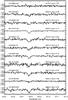 |
Fig. 1 High-resolution spectra of the Li i 670.79 nm doublet region for the 11 newly observed stars of the sample. For stars for which multiple spectra were available, the coadded spectrum is shown. For the purpose of visualization, all the spectra have been shifted to zero radial velocity and normalized. Teff increases from bottom to top, 3D scale Teff and A(Li)3D,NLTE (see Sects. 4 and 6) are listed for each star. The star CS 22882–027 shows no detectable Li line, and the 3σ upper limit to A(Li) is listed here. |
The data were reduced and analyzed with the same procedures used in Bonifacio et al. (2007), to which the interested reader is referred for details of the analysis and the associated uncertainties. An extract of the table listing the employed Fe i and Fe ii lines, in addition to associated atomic data, equivalent widths, and abundances in the 3D scale is available in Table 3. The full table is available at the CDS.
3. Atmosphere models and spectrosynthesis programs
3.1. 1D LTE models and spectrosynthesis
Various one-dimensional (1D) local thermodynamical equilibrium (LTE) atmosphere models were employed in the present study. Castelli’s grid of fluxes computed using ATLAS 9 (Castelli & Kurucz 2003)2 was used in the infrared flux temperature determination (see Sect. 4.2). A second ATLAS 9 model grid (Kurucz 2005; Sbordone et al. 2004; Sbordone 2005) was computed with an ad hoc mixing length parameter in producing the Hα-wing profiles used to determine Teff (see Sect. 4.1). It has been shown (Fuhrmann et al. 1993; van’t Veer-Menneret & Megessier 1996) that employing in ATLAS a mixing length parameter of l/Hp = 0.5 provides the best fit to Balmer lines profiles in the Sun, while the value l/Hp = 1.25 generally better reproduces more closely the solar flux, and thus, is usually employed in “general purpose” models. To compute these profiles, we employed a modified version of Kurucz’s code BALMER3, which was capable of handling different line-broadening theories. Finally, we employed OSMARCS atmosphere models (Gustafsson et al. 1975; Plez et al. 1992; Edvardsson et al. 1993; Asplund et al. 1997; Gustafsson et al. 2003) and the turbospectrum spectral synthesis code (Alvarez & Plez 1998) to determine Fe i and Fe ii abundances, gravity, microturbulence, and Li abundances. Hydrostatic monodimensional LHD models (see Caffau & Ludwig 2007; Caffau et al. 2007) were used in determining the 1D NLTE corrections (see Sect. 6.1).
3.2. 3D hydrodynamical models and spectrosynthesis
Time-dependent, hydrodynamical 3D stellar atmosphere models computed with CO5BOLD (Freytag et al. 2002; Wedemeyer et al. 2004) as part of the CIFIST model grid (Ludwig et al. 2009b)4 were employed to produce grids of Hα-wing profiles for Teff estimation (see Sect. 4.1; and Ludwig et al. 2009a; Behara et al. 2009).
4. Effective temperature
Effective temperature (Teff) is the most crucial stellar atmosphere parameter influencing Li abundance determination, Li abundances derived from the Li i 670.75 nm line being sensitive to Teff at the level of about 0.03 dex for each 50 K variation in Teff. Unfortunately, a precise determination of stellar effective temperatures is generally difficult to achieve. For F/G dwarf and subgiant stars such as those studied here, Teff is routinely estimated either from photometric calibrations (e.g., Alonso et al. 2000, 2001) or by fitting the wings of Hα with a grid of synthetic profiles of varying Teff.
Both methods are plagued by specific accuracy issues. Photometric calibrations, or the infrared flux method (IRFM), are mainly sensitive to the accuracy of the photometry available, to the details of the calibration process, and to uncertainties in the interstellar reddening estimates. On the other hand, Hα fitting is mainly sensitive to both the uncertainty in the continuum normalization across the broad line wings, and the choice of the broadening theory applied in the line synthesis (see Sect. 4.1).
In this paper, we considered four temperature estimators:
-
temperatures derived from H α-wing fitting, using 1D atmosphere models and spectrosynthesis, self broadening being treated according to Barklem et al. (2000a, b) and Starkbroadening according to Stehlé & Hutcheon (1999) (we will henceforth refer tothese temperatures as “BA temperatures”, or the “BAtemperature scale”);
-
same as BA, but using the Ali & Griem (1966) self-broadening theory (ALI temperatures);
-
temperatures derived from H α-wing fitting, using 3D model atmospheres and spectrosynthesis, Barklem et al. (2000a, b) self broadening and Stehlé & Hutcheon (1999) Stark broadening (3D temperatures, for all H α derived temperatures see Sect. 4.1);
-
temperature derived with the infrared flux method (see Sect. 4.2; as well as González Hernández & Bonifacio 2009 , IRFM temperatures).
4.1. Fitting of the Hα wings
Temperature scales based on Hα-wing fitting are affected by both observational and theoretical issues. Most high-resolution spectrographs use echelle gratings operating in high orders, which exhibit a steep blaze function. The continuum placement is thus sensitive to the accuracy with which the shape of the grating blaze function can be estimated. Such uncertainties are irrelevant when studying narrow lines observed at high resolution, but are important when a broad feature such as Hα is considered. More generally, the precision of continuum placement and of the determination of the Hα wing shape are affected by noise as well as by the possible presence of weak unrecognized features (less of a problem for metal-poor stars). Among these, the blaze function shape likely introduces the largest uncertainty.
On the theoretical side, the uncertainties are due both to the atmosphere model structure and to the physics employed in the Hα synthesis. Hα-wing self broadening can be treated with different theories, most notably those of Ali & Griem (1966), Barklem et al. (2000a,b), and Allard et al. (2008). As a general rule, Ali & Griem (1966) theory leads to a significantly lower broadening coefficient with respect to the ones derived from Barklem et al. (2000a,b) and Allard et al. (2008). A significantly higher Teff is required to reproduce a given observed profile when employing the Ali & Griem (1966) theory with respect to the other theories. With the typical parameters of the stars in our sample, and using our fitting procedure, employing Ali & Griem (1966) self broadening leads to derived Teff estimates that are higher by about 150–200 K (a difference of about 0.1 dex in Li abundance) with respect to those derived by using the Barklem et al. (2000a,b) theory. The theory by Allard et al. (2008), on the other hand, leads to Teff within a few tens of K of the Teff estimates obtained when using the Barklem et al. (2000a,b) theory. We thus restricted ourselves to using the self-broadening theory of Barklem et al. (2000a,b) (in BA and 3D temperatures) and the Ali & Griem (1966) self-broadening theory (ALI temperatures).
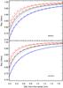 |
Fig. 2 Hα red wing profiles in the wavelength range significant for the fit. In each panel, red profiles (upper ones) are for Teff = 5400 K, black profiles (middle ones) are for Teff = 6000 K, and blue profiles (lower) for Teff = 6600 K. For each temperature, dashed profiles are for log g = 3.5, solid profiles for log g = 4.0, and dotted profiles are for log g = 4.5. All profiles assume [Fe/H] = −3. Upper panel shows profiles for BA temperatures, lower panel for ALI temperatures. |
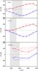 |
Fig. 3 Hα theoretical profiles for models with log g = 4, [Fe/H] = −3 (solid lines) and log g = 4, [Fe/H] = −2.5 (dot-dashed lines) have been fitted with the same procedure used for the program stars, but using a log g = 3.5 grid (red lines with filled circles) and a log g = 4.5 grid (blue lines with open diamonds). Here we plot the temperature difference (Teff(log g = 3.5/4.5) – Teff(log g = 4.0)), against the “real” effective temperature of the profile. The upper panel shows BA profiles, the middle panel ALI profiles, and lower panel 3D profiles. The gray shaded areas indicates the temperature ranges for the program stars in each Teff scale. |
The Hα-fitting temperatures exhibit a significant gravity sensitivity. Barklem et al. (2002) already reported estimates of this sensitivity for relatively metal-poor models (down to [Fe/H] = −2). The effect is always in the sense of higher gravity leading to broader profiles, and appears generally stronger at lower metallicities, at lower temperatures, and for the BA profiles compared to the ALI profiles. In Fig. 2, we plot examples of profiles for the ALI and BA cases. Profiles are plotted for Teff = 5400, 6000, and 6600 K (higher temperatures generate broader profiles). A metallicity of [Fe/H] = −3 is used. For each temperature, we plot the profile for log g = 3.5, 4, and 4.5. As can be noted, the part of the wing closest to the core appears to be more strongly affected than other parts. It is clearly seen that the gravity sensitivity of the BA profiles is roughly twice as large as in the ALI case. In both the BA and ALI scales, the gravity effect becomes quickly negligible as Teff increases above 6500 K. In the most deviant cases ([Fe/H] < −3, Teff < 6000 K, BA profiles), a difference of 0.5 dex in log g leads to roughly a 200 K difference in Teff.
Thus, the shape of the Hα profile varies in different ways when varying gravity and temperature. As a consequence, the use of an incorrect value of gravity will always affect the temperature estimate, but the size of the effect will depend on the details of how the actual fitting is performed. To provide some insight into what the effect is when employing our specific fitting procedure, we fed the fitting program with log g = 4, and [Fe/H] = −3 and −2.5 theoretical Hα profiles, and derived the temperature by assuming that log g = 3.5, 4.0, and 4.5. When fitting profiles of log g = 4.0 by means of profiles of log g = 3.5, which are narrower at each temperature, we obtain a higher temperature estimate than we would if we were to use the proper gravity. The opposite effect occurs when using the broader log g = 4.5 profiles. In Fig. 3, we plot these temperature differences versus the true Teff of the profiles. Differences are computed in the sense ΔTeff = Teff(log g = 3.5 or 4.5) − Teff(log g=4.0). Red lines with filled circles correspond to fits with log g = 3.5 profiles, blue ones with open diamonds to fits with log g = 4.5 profiles. The solid lines correspond to [Fe/H] = −3.0 profiles (both fitted and fitting), while the dot-dashed line corresponds to [Fe/H] = −2.5. For the parameter space covered, and when adopting our fitting procedure, underestimating the fitting-grid gravity by 0.5 dex leads to an overestimate of the temperature by as much as 250 K in the BA case, and 200 K in the ALI case. This underestimate reaches a maximum around 5200–5300 K, decreasing on both sides, and fading away on the hot side, near Teff = 6500 K. By overestimating the fitting-grid gravity, one underestimates Teff by as much as 300 K in the BA case and 200 K in the ALI case. The shape of the curve is similar, but the point of maximum sensitivity occurs between 5800 and 6000 K. There is a hint that the effect decreases mildly at [Fe/H] = −2.5, although higher metallicities have not been explored.
Since we estimate surface gravity from the Fe i-Fe ii ionization equilibrium, the derived gravity is temperature sensitive, so that the two estimations need to be iterated to convergence. As a general rule, we stopped iterating when Teff variations became lower than 50 K, which typically required not more than 3 iterations, starting from an initial guess of log g = 4.
A very mild metallicity sensitivity is also present in the Hαbased temperature determination, never surpassing some tens of K for a 0.5 dex of variation in [Fe/H]. The actual iteration of the temperature determination with the other atmosphere parameters was performed differently for the BA and ALI cases on one side, and for the 3D case on the other side:
-
In the BA and ALI case, once the gravity and metallicity weredetermined with one temperature estimate, theH α profile grid was interpolated to that gravity value, while the nearest grid step was chosen in metallicity, without interpolation. The small metallicity step of the grid(0.25 dex), as well as the very mild sensitivity ofH α to metallicity, made this choice sufficientlyprecise.
-
In the 3D case, the computation of both model atmospheres and spectral synthesis is very time consuming, and only the atmosphere model grids for log g = 4 and log g = 4.5 with [Fe/H] = −3.0 were sufficiently extended at the time of the analysis. We thus fitted the observed Hα lines to these two grids, deriving, for each star, effective temperatures corresponding to the two assumed gravities. We determined gravity and metallicity, then derived a new Teff estimate by linearly interpolating between the Teff(log g = 4.0) and Teff(log g = 4.5) at the estimated gravity. The procedure was then iterated but, for most stars, the same convergence criterion applied to the 1D case (ΔT < 50 K) was found to be too stringent, since the parameters for most stars ended up oscillating between two sets corresponding to Teff estimates that were about 60 K apart. This can probably be attributed to the use of a more coarse grid in the 3D case.
Coordinates and optical and infrared photometry for the program stars.
4.2. IRFM temperature estimation
Originally introduced by Blackwell & Shallis (1977), and later improved by Blackwell et al. (1980), who removed an unnecessary iteration (see Blackwell et al. 1990, and references therein), the infrared flux method (IRFM) relies on the ratio of the flux at a near-infrared (NIR) wavelength or in a NIR band, to the bolometric flux. This ratio can also be derived from model atmospheres, and the effective temperature determined by finding the effective temperature of the model that reproduces the observed ratio. González Hernández & Bonifacio (2009) presented a new implementation of the method making use of 2MASS photometry (Skrutskie et al. 2006), and also provided a calibration of bolometric fluxes with colors (V − J), (V − H), and (V − Ks), where V is in the Johnson system and the NIR magnitudes are in the 2MASS system. We applied the IRFM in exactly the way described by González Hernández & Bonifacio (2009), deriving the bolometric fluxes as the average of those estimated from the three visible-NIR colors. All magnitudes and colors used in the IRFM must be corrected for reddening. To do so, we used the reddening maps of Schlegel et al. (1998), corrected as described in Bonifacio et al. (2000). All our program stars are sufficiently distant that they lie outside the dust layer, so that the full reddening derived from the maps should be applied. The adopted reddenings are provided in Table 2. The star CS 22882–027 does not appear in the 2MASS catalog, thus we could not derive its IRFM temperature.
5. Gravity, microturbulence and metallicity
The FITLINE code was employed to measure the equivalent widths of the Fe i and Fe ii lines. Although up to ~120 Fe i lines were available, only four Fe ii lines were strong enough to be used. For each temperature scale, gravity was then derived by enforcing Fe i-Fe ii ionization equilibrium. For the Hα-based scales, gravity was used with metallicity (Fe i abundance) to iterate the Teff estimation (see Sect. 4.1).
For each temeperature scale, microturbulence was determined by ensuring that the weak and strong Fe i lines provide the same abundance. The final parameters and the derived metallicity for each temperature estimator are presented in Table 4, detailed Fe i and Fe ii abundances are listed in Table 5. Final Teff values for the ALI, IRFM, and 3D temperature scale are plotted against the BA scale in Fig. 4, and against the respective value of [Fe/H] in Fig. 5.
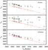 |
Fig. 4 Effective temperatures for different estimators, plotted against BA temperature for the program stars. Top to bottom: ALI, IRFM and 3D temperatures. The red line represents the one-to-one relation (hence the line of BA temperatures). |
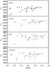 |
Fig. 5 Effective temperatures for different estimators, plotted against [Fe/H] (as derived using the temperature in the panel). Top to bottom: BA temperatures, then ALI, IRFM and 3D. |
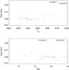 |
Fig. 6 Difference between A(Li)f and A(Li)i plotted against Teff and the Li doublet EW. The two “outliers” are labeled. |
An extract from the line-by-line Fe i and Fe ii abundance table.
Atmosphere parameters for the program stars using the different temperature estimators.
Fe i and Fe ii mean abundances, as well as their associated σ for the four temperature scales.
6. Lithium abundance determination
We determined Li equivalent widths in a similar fashion to Bonifacio et al. (2007). Synthetic line profiles were fitted to the observed profile, and the equivalent width (EW) determined from the fitted synthetic profile. The EW errors listed in Table 6 were obtained by means of Monte Carlo simulations, in which Poisson noise was added to a synthetic spectrum to ensure that it had the same S/N as the observed spectrum. The Li abundance was determined by iteratively computing synthetic spectra of the Li doublet until the synthetic EW matched the observed EW to better than 1%. The adopted atomic data were unchanged with respect to Bonifacio et al. (2007), and took account of hyperfine structure and isotopic components (a solar Li isotopic ratio was assumed). We henceforth refer to these abundances as “1D Li abundances” since Li abundances were derived using 1D atmosphere model and spectrosynthesis codes. One should avoid confusion with the 3D temperature scale, which indicates only that 3D effects have been taken into account in determining the Hα-wing fitting temperature.
In addition, we determined, for the 3D temperature scale only, what we refer to as “3D NLTE Li abundances”. As described in Sect. 6.1, a grid of time-dependent 3D NLTE spectrosyntheses have been produced for the Li i 670.8 nm doublet, and used to independently determine Li abundances from the measured EW.
The uncertainties in the Li abundance measurements were largely dominated by the uncertainty in the temperature estimation. For further details, the reader is referred to Bonifacio et al. (2007). For the purpose of our analysis, a constant uncertainty of σA(Li) = 0.09 was assumed.
6.1. 3D and NLTE corrections
We originally planned to determine the effects of both atmosphere hydrodynamics and any departure from LTE in a consistent manner, and thus computed a set of time-dependent 3D NLTE syntheses of the Li doublet over a grid of suitable 3D models, to construct a set of curves of growth (COG) for the doublet EW. Details of the computation of the 3D NLTE lithium doublet synthesis are covered in Appendix A.
Li i 670.8 nm EW and errors, and lithium abundances using the different parameter sets.
The model parameters covered by the COG grid are listed in Table 7. Once the COG grid was computed, we decided to also derive 3D NLTE lithium abundances directly, by identifying the EW-to-abundance relation that most closely fitted the computed values, and applying it to our observed EW. This was accomplished by either interpolating in the Teff, log g, [Fe/H], and EW grid (and possibly extrapolating out of it), or by determining a best fitting analytical function in the form A(Li) = f(Teff, log g, [Fe/H], EW) and applying it to the observed parameters and lithium doublet EW. We pursued both of these approaches.
We found the functional-fit method to be the superior of the two, both because of its higher accuracy and for greater ease of use. Its functional-form approach condenses the 3D NLTE abundance determination into a formula that can be hard-coded into any program, eliminating the need to carry over the true grid of computed points. Details on the fit calculation, as well as the chosen functional form and coefficients, are available in Appendix B5.
As mentioned above, we also performed an interpolation over the COG grid. The main problem in producing a suitable interpolation lies is that the grid is non-rectangular, which has two different causes. First, in the CO5BOLD hydrodynamical models Teff is not set a priori, rather, the entropy of the material entering through the bottom of the computational box is the fixed quantity. The true Teff is determined after snapshot selection, and usually varies across an interval of ± 100 K centered on the desired value for the models we employed. As a consequence, it is impossible to build a grid of CO5BOLD models with exactly the same temperature but, for example, different metallicity. Secondly, varying the stellar parameters naturally alters the relationship between A(Li) and EW, so that the range of EW in the COG corresponding to interesting values of A(Li) will vary from model to model.
Parameters of the models in the 3D CO5BOLD and 1D LHD grids used in the 3D NLTE Li abundances, and in the computation of NLTE corrections.
To simplify the task, we took advantage of the limited sensitivity of the 670.8 nm Li doublet to both gravity and metallicity. Thus, we decided to assume [Fe/H] = −3 throughout the interpolation, and to avoid interpolating in gravity by always choosing the closest value to the derived gravity between log g = 4 and log g = 4.5. This choice was also justified by the limited extension in both parameters of our sample. This reduced the problem to interpolating in an irregularly spaced two-dimensional grid in Teff and EW. Delaunay triangulation6 and quintic polynomial interpolation were then used to derive A(Li).
Figures 6 and 7 show the difference between A(Li) as determined by means of the analytical fit (A(Li)f) and by interpolation (A(Li)i), respectively, plotted against relevant quantities, on the 3D temperature scale. Most stars show an excellent concordance between the two methods, but two outliers exist, CS 29516–028 and CS 22888–031. These two stars have the lowest temperatures among all the stars in the sample (these temperatures are still within the computed grid). However, they also have the highest gravity in the sample, which requires extrapolation, since the grid has a limiting gravity of log g of 4.5. While the functional fit is indeed extrapolated, the simplified interpolation assumes log g = 4.5 in this instance; the discrepancy between the two methods does not however exceed 0.023 dex in A(Li), which is negligible for our purpose. All the remaining stars exhibit discrepancies not exceeding 0.01 dex.
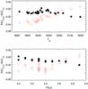 |
Fig. 8 The NLTE correction (A(Li)1D,NLTE – A(Li) 1D,LTE), computed for each star using our model atom (black filled dots) along with the Carlsson et al. (1994) values (red open circles), plotted against Teff and log g. The 3D temperature scale is assumed. |
A parallel grid of COG was produced using LHD models sharing the same parameters as the CO5BOLD ones. The 1D syntheses were produced both including and neglecting NLTE effects, for the specific purpose of deriving a grid of NLTE corrections applicable to our 1D Li abundances. For comparison, Fig. 8 shows our 1D NLTE corrections (for the 3D temperature scale) versus Teff and log g, together with the corresponding values obtained by using the Carlsson et al. (1994) NLTE corrections, while Fig. 9 shows a similar comparison using the updated calculations by Lind et al. (2009a). Since Lind et al. (2009a) corrections are defined down to [Fe/H] = −3, in Fig. 9 [Fe/H] = −3 is assumed for all stars both in computing our NLTE correction and in computing those based on Lind et al. (2009a) scale. Trends with effective temperature and gravity are extremely similar for our corrections and those of Lind et al. (2009a), but a very uniform offset of about 0.03 dex is present between the two set of corrections. The origin of this offset is probably the different sets of underlying atmosphere models. Since the offset is quite uniform across the sample, using either set of corrections is of no consequence on the scientific output of the present work.
7. Results
We decided to adopt the 3D temperature scale (and its derived parameters) together with the 3D NLTE Li abundance set as our preferred values, and henceforth, when not otherwise specified, we will refer to these.
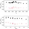 |
Fig. 9 The NLTE correction (A(Li)1D,NLTE – A(Li) 1D,LTE), computed for each star using our model atom (black filled dots) along with the Lind et al. (2009a) values (red open circles), plotted against Teff and log g. The 3D temperature scale is assumed, and [Fe/H] = −3 is imposed for all stars. |
7.1. Sensitivity to the adopted Teff scale
One of the most remarkable results of this work is that, although the choice of temperature scale alters the parameters and derived Li abundance of the stars, it does not change the general picture that emerges. Table 8 provides the results of Kendall’s τ-test and the slopes of linear fits to the A(Li)-[Fe/H] and A(Li)-Teff relations. The linear fits were obtained taking into account errors in both variables using the fitexy routine (Press et al. 1992). The A(Li) error was assumed to be fixed at 0.09 dex, the error in [Fe/H] to be given by the Fe i line-to-line scatter for each star, and the error in Teff to have a constant value of 130 K. The sample consists of 27 of the 28 stars for which we have Li measurements, excluding CS 22882–027, for which we only have an upper limit to A(Li), as well as CS 21188–033, where the residuals from the best-fit regressions are on the order of 3–4σ.
In statistical terms, for all four temperature scales a non-parametric Kendall’s τ-test indicates that A(Li) correlates with [Fe/H] at a very high level of significance (see Table 8). Moreover, a linear fit to the A(Li)-[Fe/H] relation on the different temperature scales produces slope values that are both always significant at the level of 3σ and, strikingly, consistent with each other within 1σ. The slope values are also the highest reported to date. The hypothesis that the “slope” in the A(Li)-[Fe/H] relation might be due to the specific Teff scale chosen can thus be safely rejected.
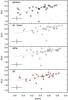 |
Fig. 10 Li abundance versus [Fe/H] for the four temperature estimates. Top to bottom, BA, ALI, IRFM, and 3D temperatures. For the 3D temperature scale, the black triangles represent the 3D NLTE Li abundances, while the red crosses represent 1D LTE Li abundances with the NLTE corrections applied. The best-fit linear relation (as per Table 8) is indicated by a gray line. A typical error bar of ± 0.09 dex in Li abundance and the average [Fe/H] error bar are also displayed. |
7.2. The meltdown of the Spite plateau: slope or scatter?
Three different Hα-based Teff scales, as well as the totally independent IRFM scale, concur in indicating that the Spite plateau is disrupted below [Fe/H] ~ −3 (see Fig. 10). Close to that metallicity, one observes a significant increase in the Li abundance scatter, which appears to act always towards lower abundances. In other words, while some rare stars persist at the plateau level even at very low metallicity (CS 22876–032 A, González Hernández et al. 2008), the vast majority exhibit some degree of Li “depletion” (with respect to the plateau value).
Two stars in the sample exhibit anomalously low Li abundances. The star CS 22188–033 exhibits a mild Li depletion with a 3D NLTE A(Li) = 1.66, while CS 22882–027 has no detectable Li doublet (see Sect. 7.5).
One of the much-debated results concerning the behavior of Li abundances in metal-poor halo dwarfs has been the reported existence of a correlation between A(Li) and [Fe/H], since it was first reported by Ryan et al. (1999). We investigated this by means of two different statistical tests. The Kendall’s τ rank-correlation test attempts to detect a (positive or negative) correlation, and has the fundamental strength of being non-parametric. In other words, it does not attempt to look for a specific relation to fit the data. As seen above, Kendall’s τ-test quite strongly supports the existence of a correlation.
The other obvious strategy we adopt is to fit the data with a linear function and see whether the slope found is statistically significant. This significance might be weakened if the data are indeed correlated, but the underlying relation is not linear. In our case, again, the slope of the linear relation is significant at 3σ for all the considered temperature scales. This a finding, however, does not imply that the underlying “physical” relation between [Fe/H] and A(Li) is linear, as it would be, for example, if there was a constant Li production with increasing [Fe/H].
To shed more light on the issue, in Fig. 11 we plot the residuals of the best-fit A(Li) versus [Fe/H] relation, as listed in Table 8. An increase in the scatter below [Fe/H] ~ −2.8 was already visually apparent in Fig. 10, and remains clearly recognizable in Fig. 11 once the best-fit linear relation is subtracted. To provide quantitative estimates of the level of scatter, we divided the sample into two in terms of metallicity, a metal-richer subsample including the 8 stars with [Fe/H]3D > −2.8, and a metal-poorer sub-sample including the 19 stars below that threshold. The star CS 22188–033 is plotted in the figure, but it has not been considered in this computation. We then computed the dispersion in the residuals of the two subsamples for the four temperature scales: σhi,BA = 0.04 dex, σlo,BA = 0.10 dex; σhi,ALI = 0.05 dex, σlo,ALI = 0.08 dex; σhi,IRFM = 0.02 dex, σlo,IRFM = 0.10 dex; σhi,3D = 0.05 dex, σlo,3D = 0.09 dex. For every temperature scale, the scatter in the residuals is about twice as large (or more) below [Fe/H] = −2.8 than above. It is thus clear that the tight, flat relation that is known as the Spite plateau develops both a tilt and a significant scatter at low metallicities. Once again, it is remarkable how the level of scatter appears independent of the assumed temperature scale.
We note that the true Li doublet EW does not change much with metallicity, since in general A(Li) does not vary by more than 0.2 dex. The quality of the Li doublet measurement is thus roughly constant across the whole metallicity range. The increase in scatter thus cannot be attributed to the declining quality of the measurements. On the other hand, Fe i and Fe ii lines do become weaker with metallicity, which lowers the quality of the gravity estimation. Since the Hα line is quite gravity sensitive, inaccurate gravities reflect directly on Hα-based Teff estimations, and thus on A(Li). On the other hand, the IRFM temperature scale is totally insensitive to this effect, and yet shows the largest increase in the scatter of its residuals, and a low-metallicity scatter equal to those of the Hα-based Teff scales. This reinforces our impression that the increase in the A(Li) residual scatter should indeed be real.
7.3. Plateau placement
As a consequence of what is said above, it hardly makes sense to provide an average value
for A(Li) in our stars. One might still try, however, to determine the
position of the plateau for the more metal-rich stars of the sample, which still appear to
fall onto it. Every operation of this kind is somewhat arbitrary, since there is no
clear-cut transition between the plateau at higher Fe content and the sloping/dispersed
distribution at low metallicity. We thus decided to employ the 9 stars whose metallicity
is equal or greater than −2.8 in the 3D scale, and consider their
A(Li) and dispersion as being representative of the Spite plateau. The
resulting values are 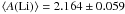 in the BA scale,
 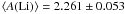 in the ALI scale,
 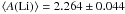 in the IRFM scale, and
  using A(Li)3D,NLTE together with the 3D
temperature scale.
using A(Li)3D,NLTE together with the 3D
temperature scale.
7.4. The A(Li) – Teff correlation
In Fig. 12, as well as in Table 8, a positive slope of Li abundance with effective temperature is present in all the temperature scales. It is, however, remarkable that this slope is driven by the coolest stars. Adopting our 3D temperature scale, if we select only the stars hotter than 6250 K (22 stars), the slope essentially vanishes, the probability indicated by Kendall’s τ drops to 89%, and a parametric test does not detect any slope.
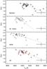 |
Fig. 12 Li abundance versus effective temperature for the four temperature estimates. Symbols are the same as in Fig. 10. Typical error bars of ± 0.09 dex in the Li abundance and ± 130 K in Teff are also displayed. The best-fit linear relation as per Table 8 is indicated by a gray line. |
Given the very small population of this temperature range in our sample, it is possible that we just missed any undepleted cool object. On the other hand, this might suggest that the decline (caused by convection) usually seen for stars cooler than ~5700 K at higher metallicities may set in at higher temperatures for EMP stars (although observationally the opposite seems to be true, see Boesgaard et al. 2005).
We emphasize, however, that the depletion of the cool end of the sample is not driving the A(Li)-[Fe/H] correlation: removing the aforementioned five cool stars has a negligible effect on this result. On the 3D scale, the Kendall’s τ correlation probability of A(Li)3D,NLTE with [Fe/H] passes from 0.999 to 0.998, while the slope of the linear fit goes from 0.274 ± 0.083 to 0.253 ± 0.086 when these 5 stars are removed. This is because the cool stars, while appearing to be all Li depleted, are evenly distributed in metallicity between [Fe/H] ~ −3.2 and -2.8. On the other hand, removing these stars would affect the detected increase in the scatter at lower metallicities: applying the same residual analysis mentioned in Sect. 7.2, but now on the hot stars only, would yield σhi,3D,hot = 0.04 dex (was 0.05 with the full sample), and σlo,3D,hot = 0.06 dex (was 0.09 with the full sample).
7.5. CS 22882–027 and HE 1148–0037
Two additional stars were included in the original sample, but Li abundance has not been computed for them, for different reasons. We elaborate briefly on these objects.
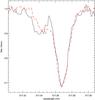 |
Fig. 13 The Mg i 517.268 nm line for HE 1148–0037, in spectra taken at JD 2 453 787.6803 (black continuous line) and JD 2 453 823.5443 (red dashed line), separated by 35.86 days. The spectra have been normalized, and Doppler shifted to bring the primary component to a rest-frame wavelength. The binarity is readily visible, as well as the variation in the components’ separation. |
Atmospheric parameters and metallicity were computed for CS 22882–027 (see Table 4), but the star has no detectable Li doublet (see Fig. 1). Given a S/N ~ 80, as measured in the Li doublet range, a typical line FWHM of 0.033 nm, and a pixel size of 0.0027 nm, the Cayrel (1988) formula predicts that a Li doublet of EW = 0.563 pm would be measured at 3σ confidence (1σ = 0.187 pm). Employing our fuctional fit, this leads to an upper limit of A(Li)3D,NLTE ≤ 1.82, assuming an EW = 0.563 pm and A(Li) 3D,NLTE ≤ 1.34, assuming EW = 0.187 pm. We have a single-epoch spectrum for this star that shows no sign of a double-line system.
The star HE 1148–0037 was also originally included in the sample, but immediately set aside, since from visual inspection of the two available spectra it turned out to be a double-lined binary system. As shown in Fig. 13, the two spectra, separated by 35.86 days, clearly exhibit evidence of the double-line system, as well as readily recognizable variation in the separation between the two line systems. We were able to retrieve 3 spectra of HE 1148–0037, and measure radial velocities for the two components, which are given in Table 9, by means of cross-correlation against a synthetic template (Teff = 6000 K, log g = 4.0, [Fe/H] = −2.0). In our two spectra (2006-02-21 and 2006-03-29), cross-correlation was computed in the 490–570 nm range. We also had the lower resolution, blue-range only HERES spectrum, which was used to derive the Vrad after masking all the broad hydrogen lines. Internal errors of the radial velocity estimate were evaluated by performing a Monte Carlo test on a sample of 50 simulated binary star spectra with noise added to emulate a S/N = 90, the component separation and resolution being equivalent to that of the March 29, 2006 observation. The test inferred an average error of 0.072 km s-1 for the primary component and 0.246 km s-1 for the secondary. These values are representative of the internal errors in the cross-correlation procedure, but are surely dominated by the spectrograph zero-point calibration uncertainty, which was not taken into account particularly well, because very precise radial velocities were not among the goals of this study. We thus list in Table 9 an estimated total error of 1 km s-1 for all our observations, which we take to be representative of the overall systematics of these measurements.
On the other hand, Aoki et al. (2009) report AN uncertainty given by the internal scatter in the radial velocities obtained from different lines; they do not take into account the systematic uncertainties in the wavelength calibration, hence the much lower value of uncertainty. In Table 9, we kept the value they provide, but we propose that the true uncertainty is again close to 1 km s-1. If we consider their measure to be representative of the primary component radial velocity, it reproduces well the three other measurements we present.
Barycentric radial velocities for the two components of the binary system HE1148–0037 as measured from the spectra available to us.
7.6. Comparison with other results
Our most significant overlap is of course with the Bonifacio et al. (2007) sample, of which the present study represents a continuation. Of the 19 stars in Bonifacio et al. (2007), 17 were reanalyzed here (the two remaining stars, BS 16076–006 and BS 16968–061 turned out to be subgiants and have thus been dropped). Bonifacio et al. (2007) determined Teff by fitting the Hα wings fits with profiles synthesized using the Barklem et al. (2000a,b) self-broadening theory. Their temperature scale thus closely resembles our BA scale, but the Hα gravity sensitivity was not taken into account in that study – log g = 4.0 was assumed in computing the profiles. The effect is clearly visible in Fig. 14. The upper panel of this figure plots the temperature difference, Teff(this work) − Teff(Bonifacio et al. 2007), against the Bonifacio et al. (2007) gravity estimate. It is immediately evident that, for stars around log g = 4.0, the temperature difference approaches zero. For stars at higher gravities, our Teff estimate is below the Bonifacio et al. (2007) value by up to 200 K. This reflects the behavior presented in Fig. 3: when a profile is fitted with a synthetic grid computed for a gravity that is underestimated, this leads to an overestimated Teff. We note that Fig. 14 does not tell the entire story. As we do here, Bonifacio et al. (2007) estimated log g by enforcing Fe ionization equilibrium, so the derived gravity values are not identical in this work and Bonifacio et al. (2007). High-gravity and low-gravity stars do, however, retain their approximate placement in both cases, although the gravity span can be somewhat stretched by the Teff bias. The effect of the Teff difference on [Fe/H] is shown in the middle panel of Fig. 14, while in the lower panel the difference between A(Li) for the same stars is plotted, considering here the LTE values (to eliminate the effect of the marginally different NLTE corrections applied in the two works). The results shown are to be expected, given the strong Teff sensitivity of the Li i 670.8 nm doublet: the current A(Li) is higher by up to about 0.1 dex for low-gravity stars, while it is lower by roughly the same amount for high-gravity stars. On the other hand, it is easy to see how the discrepancy will only marginally affect a linear fit of A(Li) versus [Fe/H]: the stars are displaced roughly along a 1:1 diagonal in the A(Li)–[Fe/H] plane.
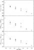 |
Fig. 14 Comparison between the results of this work and of Bonifacio et al. (2007) for the 17 stars in common. In the upper panel, the difference between our Teff and the Bonifacio et al. (2007)Teff determination is plotted against the value of log g in Bonifacio et al. (2007). In the center panel, we show [Fe/H] difference, and in the lower panel, the difference in the A(Li) LTE. For our results, BA temperature scale is used. |
The star LP 815–43 is the only object that overlaps with the Asplund et al. (2006) sample. In that work, effective temperature is measured again by fitting Hα wings with a set of synthetic profiles. The details of the fitting procedure differ somewhat and the synthetic profiles are computed from MARCS models using the BSYN synthesis code. The Barklem et al. (2000a,b) self-broadening theory is assumed here for Hα, so again the BA scale is the one to be used in the comparison. The Hα gravity sensitivity is taken into account here, and the derived Teff is quite close to our value (6400 K vs. 6453 K in this work). Asplund et al. (2006) determine metallicity from Fe ii lines, and gravity from Hipparcos parallaxes, but again the values do not differ much from our results (log g = 4.17, Vturb = 1.5, [Fe/H] = − 2.74). The residual 0.14 dex offset in metallicity is in good agreement with the 0.2 dex offset detected by Bonifacio et al. (2007) between their metallicity scale and that of Asplund et al. (2006). The lithium abundance is again quite close to our result: from the 670.8 nm doublet, they derive A(7Li) = 2.16, while our value is 2.23. The difference is fully accounted for once the Teff effect is considered (0.03 dex) as well as the already known, albeit still unexplained, 0.04 dex bias between A(Li) as derived by means of BSYN and turbospectrum (Bonifacio et al. 2007).
The same star is also in common with Hosford et al. (2009). That work uses excitation equilibrium to estimate Teff, a method that is not directly comparable with any of our temperature scale. The authors derive two parameter sets, one assuming the star belongs on the main sequence, and another assuming it is a subgiant. In the first case (Teff = 6529, log g = 4.40, Vturb = 1.4, [Fe/H] = − 2.61), they obtain a temperature that is only about 50 K cooler than for our 3D and ALI scale, but a higher gravity and metallicity. In the second case (Teff = 6400, log g = 3.80, Vturb = 1.4, [Fe/H] = −2.68), they derive a temperature 50 K cooler than for our BA scale, the same gravity, but again to a metallicity 0.2 dex higher. Their measured Li doublet equivalent width is about 0.2 pm smaller than that we find, and in both cases they derive an A(Li) that is about 0.1 dex smaller than ours. This is consistent with the expected combined effect of the difference in both Teff and the Li doublet EW.
Three stars are in common with the Aoki et al. (2009) sample, but we determined A(Li) for only two of them, CS 22948–093 and CS 22965–054. Aoki et al. (2009) employ Hα- as well as Hβ-wing fitting to determine Teff on the basis of MARCS models and using the Barklem et al. (2000a,b) self-broadening for Hα. Once more, our BA temperature scale is the one most appropriate for a comparison. The Hα gravity sensitivity is taken into account. Surface gravities are estimated by comparing with isochrones as well as by evaluating the Fe i–Fe ii ionization equilibrium. The parameter values they derive for CS 22948–093 are in close agreement with those we derive (Teff(Hα) = 6320 K, Teff = 6380, log g = 4.4, Vturb = 1.5), while [Fe/H] is 0.13 dex lower at −3.43. The derived value of A(Li)LTE = 1.96 is inexcellent agreement with our value of 1.935. CS 22965–054 shows a more significant discrepancy in Teff. Their value of Teff(Hα) = 6390 K is remarkably higher than our, while Teff(Hβ) is much closer to our value. Since the adopted temperature is the average of the two, the final Teff is ultimately just 56 K hotter than our value. Their derived surface gravity is also very close in value (log g = 3.9), while Vturb is the same. However, Aoki et al. (2009) derive the same lithium abundance as we do, A(Li)LTE = 2.16, due to their lower measured value of EW (2.03 pm) for the Li doublet.
The third star in common with Aoki et al. (2009) is HE 1148–0037, for which Aoki et al. (2009) do not appear to have noticed its binarity. On close inspection, the single spectrum they employed (JD 2 453 428.94) shows signs of line asymmetry (Aoki 2009, priv. comm.), but it appears to have been taken quite close to conjunction. In contrast, as seen in Sect. 7.5, the three spectra we have of this star all show quite clearly the two line systems.
We observed No star in common with Meléndez &
Ramírez (2004). A comparison with their sample is nevertheless interesting due to
the extension of their sample to very low metallicities, despite with a limited number of
stars (a total of 10 stars were analyzed below [Fe/H] = −2.5, 4 at or below [Fe/H] =
− 3). Meléndez & Ramírez (2004) detected
no slope in the Spite plateau, for which they advocated a high value of
 .
As noticed in González Hernández & Bonifacio
(2009), the Teff scale adopted by Meléndez & Ramírez (2004) is systematically
hotter than the one we employ for metal poor dwarfs, on average by 87 K. This explains
half of the descrepancy between our average IRFM plateau placement and their own, and can
account in principle for their failure to detect the slope, assuming their temperature
scale and ours diverge progressively at low metallicities.
.
As noticed in González Hernández & Bonifacio
(2009), the Teff scale adopted by Meléndez & Ramírez (2004) is systematically
hotter than the one we employ for metal poor dwarfs, on average by 87 K. This explains
half of the descrepancy between our average IRFM plateau placement and their own, and can
account in principle for their failure to detect the slope, assuming their temperature
scale and ours diverge progressively at low metallicities.
Lithium abundances for two extremely metal poor stars (HE 0233–0343 and HE 0945–1435) were recently presented by García Pérez et al. (2008). Both stars show extremely low Fe content ([Fe/H] ~ −4), but probably because of the weakness of Fe ii lines, the estimation of gravity is uncertain. This affects the determinations of both the evolutionary status (either MS or early SGB) and Teff, which is derived from Hα wing fitting in a way similar to that used with our BA scale. The stars appear to be fairly cool, 6000 K ≤ Teff ≤ 6250 K, which would place them among the “cool stars” of our sample as described in Sect. 7.4, and both objects show significantly depleted Li, A(Li) ~ 1.8. Owing to the uncertainty of the parameters determination we did not include these stars in Fig. 15.
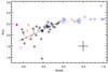 |
Fig. 15 A unified view of A(Li) vs. [Fe/H] from some studies for which a common temperature scale can be assumed. Blue circles, Asplund et al. (2006) data, red triangles, Aoki et al. (2009) data, magenta squares, CS 22876–032 from González Hernández et al. (2008), filled symbol primary star, open symbol secondary star. Black diamonds, this work, BA temperature scale. Dot-dashed gray line, best linear fit to Asplund et al. (2006) data, continuous dark gray line, best fit to our data. Typical error bars for our data are displayed. |
8. Possible biases
8.1. Binary stars
Two potential biases can, in principle, be responsible for producing systematically low Li abundances, and a trend of A(Li) with metallicity. The first one is of course the presence of undetected binaries, for which the veiling by the secondary star will systematically reduce the EW of the lines of the primary, leading to an underestimate of both metallicity and Li abundance. The true impact of this effect is difficult to evaluate, mainly because little is known about the fraction, and mass-ratio distribution, of binaries at low metallicities. Duquennoy et al. (1991) report, for G dwarfs in the solar vicinity, a fraction of 44% of stars having a companion with q = M2/M1 > 0.1, about 1/3 of which have q > 0.5. Latham et al. (2002, and references therein) found that the halo binary population does not differ significantly from the disk one, although we note that they did not explore significant numbers of stars with metallicities as low as the stars in our present sample.
It nevertheless seems unlikely that undetected binaries pollute our sample significantly. We checked for binarity by inspecting the Mg b triplet lines (e.g., see Fig. 13). Our spectra have a typical S/N ~ 100 or higher, and Mg b lines have a typical EW of 10 pm. A line with central residual intensity of 0.95 would be detected at least at the 5σ level in this typical spectrum, and have a typical EW of 0.8 pm. As per González Hernández et al. (2008), to reduce a 10 pm line to 0.8 pm, a ratio of the continua fluxes of about 11.5 is needed. If we roughly assume that the total luminosity scales accordingly, this corresponds roughly to q = 0.5 (since L ∝ M3.2 on the main sequence, see Kippenhahn & Weigert 1990). A similar flux ratio in the Li doublet range would lead to a correction of the Li doublet EW for the primary star of about 8%, corresponding to 0.03 dex in A(Li). In other words, every binary star requiring significant veiling correction on the primary spectrum would also be promptly detectable because of the double line system. This system could only stay undetected if the radial velocity separation of the two stars was quite small at the moment of the observation(s), so that the two line systems remained blended.
In addition to the above, if we take the figures of Duquennoy et al. (1991) at face value, find that about 13.5% of the binaries are characterized by a significant veiling of the primary (i.e. q > 0.5). Our original sample comprised 30 stars, which implies that there are 4 expected “significant binaries”. Three stars have already been rejected from the sample, one of them (HE 1148–0037) being indeed a binary. Two more (CS 22882–027 and CS 22188–033) exhibit significant lithium depletion or no Li doublet at all, and were excluded from all statistical analyses. They are clearly the most likely candidates to be binaries, albeit neither one shows a double line system7. One could thus expect one more “disguised” binary to be biasing the sample. While this is quite possible, it would hardly influence any of our results.
8.2. 3D NLTE effects on Fe ionization equilibrium
The second problem relates to the use of Fe i-Fe ii ionization equilibrium to estimate gravity. From preliminary computations, it appears that 3D corrections of Fe lines with excitation potentials of the same order as employed in the present work could be quite large at low metallicities for stars similar to those that we study. Moreover, corrections for Fe i appear to be negative (of about 0.2 dex), while they are positive (about 0.1 dex) for Fe ii lines, for a Teff = 6500, log g = 4.5, [Fe/H] = −3.0 star. The phenomenon is mainly caused by the overcooling that 3D treatment produces in the outer layers of atmospheres at low metallicities, and appears to be of similar magnitude at [Fe/H] = −2 (due to the stronger saturation of Fe lines, which drives their contribution function to higher layers), but would most likely disappear above. If taken at face value, a 0.3 dex Fe i-Fe ii imbalance would lead to an overestimate of log g of about 0.5 dex when analyzed using 1D LTE models (as is our case regarding metallicity and gravity estimation). We do indeed find higher gravities than expected from evolutionary tracks. On the other hand, we do not currently have a 3D NLTE spectrosynthesis code for iron; we are thus unable to account for NLTE effects, which are likely to counterbalance the 3D effect because of over-ionization occurring in the upper layers where overcooling is present in 3D models. A similar mechanism is indeed active for Li, whose 3D LTE abundance derived by CO5BOLD-LINFOR3D is about 0.2 dex below the corresponding 1D NLTE value, while the 3D NLTE one is essentially indistinguishable from the 1D NLTE result (Figs. 10 and 12). If some degree of imbalance remains after NLTE is taken into account, and is metallicity sensitive, this might introduce a bias when Teff is determined by Hα-wing fitting. It is indeed intriguing to note how lower gravity estimates lead to higher temperatures, and as a consequence, (somewhat) higher the Li abundances. On the other hand, the IRFM temperature scale should be immune to this problem, A(Li) being quite insensitive to log g itself, and the IRFM-based analysis inferring abundances similar to the Hα-based estimate.
9. Conclusions
We have presented the largest sample to date of Li abundances for EMP halo dwarf stars (27 abundances and one upper limit), including the largest sample to date below [Fe/H] = −3 (10 abundances). Lithium abundance determination is highly sensitive to biases in the effective temperature scale, and we have tried to account for this using four different temperature estimators. In an additional effort to accurately represent the stellar atmospheres of the sample stars, 3D, time-dependent, hydrodynamical atmosphere models have been used to determinine our preferred Hα-based temperature scale, and a detailed 3D NLTE spectrosynthesis has been applied to the determination of lithium abundance. Both these techniques have been employed here for the first time, to our knowledge, in the analysis of EMP stars. This has also allowed us to develop a useful fitting formula allowing one to derive A(Li)3D,NLTE directly as a function of EW, Teff, log g, and [Fe/H] for EMP turn-off and early subgiant stars (see Appendix B).
The first obvious conclusion of this work is that we have confirmed what was merely suggested by the analysis of Bonifacio et al. (2007), and previous works, that at the lowest metallicity there is sizable dispersion in the Li abundances and that there is a trend of decreasing Li abundance with decreasing metallicity. We have also shown that these two conclusions do not depend on the adopted temperature scale, as suggested by Molaro (2008). The results hold, qualitatively, using both IRFM temperatures and Hα temperatures, regardless of the broadening theory adopted and irrespective of the use of either 1D or 3D model atmospheres. Quantitatively, the results differ in the mean level of the Li abundance, while the slopes in the A(Li) versus [Fe/H] relations agree within errors. None of the temperature scales investigated produces a “flat” Spite plateau over the full range in [Fe/H] (see Table 8).
Our results are in substantial agreement with those of Aoki et al. (2009). While these authors do not detect a slope with either effective temperature or metallicity, this happens simply because of the small extent of their sample in both these parameters. On the other hand, they do point out that their sample has a lower Li abundance than that observed at higher metallicities.
The picture outlined by the aforementioned results acquires more significance, once we place it in a broader context among the latest studies regarding lithium in EMP stars. Figure 15 compares our results with those of three investigations employing compatible temperature scales. In this figure, open blue circles represent stars from the Asplund et al. (2006) sample, red triangles from the Aoki et al. (2009) data, and the two magenta squares the two components of the double-lined binary system CS 22876–032 (González Hernández et al. 2008, the filled square corresponds to the primary star). Our data are represented as black diamonds (the results of the BA scale are shown, for compatibility with the temperature scales used in the other three works)8. The best linear fit to our data is shown as a dark gray solid line, while the best fit to Asplund et al. (2006) data (A(Li) = 2.409 + 0.103[Fe/H]) is shown by a dot-dashed gray line. The Asplund et al. (2006) Li abundances are increased here by 0.04 dex to account for the known offset already mentioned in Sect. 7.6, and their metallicty is decreased by 0.2 dex to correspond to the metallicity-scale offset detected by Bonifacio et al. (2007). It is now even more evident that the Spite plateau does not exist anymore at the lowest metallicity, and is replaced by an increased spread of abundances, apparently covering a roughly triangular region ending quite sharply at the plateau level. This region appears here to be populated in a remarkably even manner; at any probed metallicity some star remains at, or very close to, the Spite plateau level, but many do not. The rather different slopes of the best-fit relations in Asplund et al. (2006) and in this work appear to be the obvious consequence of fitting two subsamples covering different metallicity regimes. This could provide also an explanation for the numerous claims, starting from Ryan et al. (1999), of a thin, but tilted Spite plateau. From this view, the difference was produced simply because the tail of these samples had been falling in the low-metallicity “overdepletion zone” as we have been able to discern more clearly.
We are not aware of any theoretical explanation of this behavior. After the measurements of the fluctuations of the CMB made it clear that there is a “cosmological lithium problem”, i.e., the Li predicted by SBBN and the measured baryonic density is too high with respect to the Spite plateau (by about 0.6 dex for our sample), there have been many theoretical attempts to provide Li-depletion mechanisms that would reduce the primordial Li to the Spite plateau value in a uniform way. Our observations now place anadditional constraint on these models – below a metallicity of about [Fe/H] = −2.5, they should cause a dispersion in Li abundances and an overall lowering of A(Li).
If Li depletion from the WMAP-prescribed level were to happen in the stellar envelopes of very metal-poor stars, the mechanism would have to be remarkably metallicity insensitive to account for the thin, flat plateau observed between [Fe/H] = −2.5 and −1. And yet, the same phenomenon must become sharply metallicity sensitive around and below [Fe/H] = −2.5, i.e., precisely where metallicity effects on the atmospheric structure are expected to become vanishing small.
We are tempted to imagine that two different mechanisms may need to be invoked to explain the production of the Spite plateau for stars with [Fe/H] > −2.5, and of the low-metallicity dispersion for stars with [Fe/H] < −2.5. One could envision such a two-step process as follows:
-
1.
Metal-poor halo stars are always formed at the Spite plateaulevel, regardless of their metallicity. Whether the plateaurepresents the cosmological Li abundance or is the result of someprimordial uniform depletion taking place before the starformation phase is immaterial in this context.
-
2.
A second phenomenon, possibly related to atmospheric diffusion, becomes active around [Fe/H] = −2.5 and below, depleting Li further in the atmosphere of EMP stars. This phenomenon, aside from the metallicity sensitivity, would exhibit different star-to-star efficiency, being possibly dependent on additional parameters, such as stellar rotation or Teff. Its efficiency must in any case be higher for more metal-poor stars.
In this scenario, the “primordial” plateau would be preserved above [Fe/H] ~ −2.5, but below that metallicity, a systematic “leakage” of stars towards lower A(Li) would take place, more effectively for more metal-poor stars, but naturally scattered due to the sensitivity to parameters other than [Fe/H]. This scheme would have a number of advantages. First of all, it would naturally explain our observations, “mimicking” a slope in A(Li) versus [Fe/H], but with increased scatter at low [Fe/H]. It would also explain why, while the scatter in A(Li) increases at low metallicities, not a single star in this metallicity regime has been found to lie above the Spite plateau level. It would then be consistent with a small number of stars remaining close to the plateau at any metallicity (e.g., CS 22876–032 A, González Hernández et al. 2008,filled magenta square in Fig. 15); in these objects, the depletion process would be somehow inhibited. Finally, attributing the extra depletion to atmospheric diffusion/settling would not require a physical “conspiracy” capable of producing exactly the same depletion level regardless of metallicity, stellar rotation, gravity, or effective temperature, as is often invoked when diffusion is used to explain the Spite plateau.
The nature of what we refer to above as the “second phenomenon”, the one responsible for the departures from the Spite plateau below [Fe/H] = −2.5, is perhaps the most intriguing. Above, we have proposed some kind of photospheric settling mechanism, but one could as well envision a chemical evolution scenario, on the basis of some gas pre-processing with Li depletion (à la Piau et al. 2006) – while it may not be able to account for the entire WMAP-Spite plateau discrepancy, this mechanism could easily account for the mild (0.2–0.4 dex) departure from the plateau observed at lower metallicities. Moreover, this mechanism would naturally produce a spread of abundances as a consequence of the local level of gas pre-processing.
There are hints that the recently discovered ultra-faint dwarf galaxies (uFdg) might have been the source of the bulk of the EMP stars now found in the halo of the Milky Way (Tolstoy et al. 2009, and references therein). If this were indeed the case, a sizeable fraction of our sample could have formed in uFdg systems, possibly more so for the most metal-poor objects. It has been suggested (Komiya et al. 2009) that the paucity of stars below [Fe/H] = −3.5 may be due to the onset of self-pollution in the primordial mini-halos when they started to merge to form larger structures, and ultimately the halo. One could then envision that gas reprocessing could have fairly significantly altered the Li abundances in the heavily dark-matter dominated cores of these sub-halos, but become progressively negligible when they merged, and their ISM mixed more and more completely with gas of pristine Li abundance. Sub-plateau stars may then originate from star formation that occurred in the sub-halo cores, or while mixing with pristine gas that progressively diluted the effect of the reprocessing.
In any case, the main drawback of this two-phenomena scenario is to leave the WMAP-Spite plateau discrepancy unexplained. It also implies that any depletion from WMAP-based primordial A(Li) should have taken place before the currently observed stars formed. Non-standard primordial nucleosynthesis thus remains entirely viable, until the contrary is proven.
Looking retrospectively at the history of the abundances of light elements and SBBN, one concludes that if the Spite plateau is the result of significant uniform Li depletion among metal-poor stars, one faces a formidable case of cosmic conspiracy. It is necessary to admit that the Li has been depleted quite precisely to a level consistent with SBBN production and also consistent with the abundances of the other measurable light elements. Had Li been depleted to the level of A(Li) = 1.8, that is, below the minimum allowed by SBBN, the Spite plateau might not have been interpreted as being related to primordial Li, right from the beginning.
A caveat is in order when looking at Fig. 15: the Asplund et al. (2006) sample is biased, having been purposedly selected not to include objects significantly deviating from the Spite plateau. In fact, stars with varying degrees of Li depletion have long been known to exist (e.g., Charbonnel & Primas 2005). On the other hand, warm (i.e., Teff > 6000 K) dwarf stars deviating from the Spite Plateau appear to be quite rare at [Fe/H] > −3. Again, our sample is limited towards higher metallicities, which prevents us from properly quantifying this statement. A re-evaluation of the Li abundances above [Fe/H] = −2.5 is in order, using an analysis technique homogeneous with the present one, and applied to a sample for which a well-known selection technique has been applied. It is plain to see that, had previous authors encountered Li abundance distributions as the one observed by us and Aoki et al. (2009), the concept of a lithium abundance plateau would have been short lived. Instead, there is a clear perception that mildly Li depleted stars do exist among MP stars, but are a rare occurrence. We cannot easily identify any reason why all the previous studies should have been biased in a different way with respect to the present one, but until a coherent work, based on a well defined selection criterion, is extended to higher metallicities, all we are left with is just this perception.
Two other lines of future investigation are suggested by the present results: (i) increase the sample of hot (Teff ≥ 6250 K)) EMP stars ([Fe/H] ≤ −3.0), and (ii) increase the number of cool (Teff < 6250 K) stars over the entire metallicity range. The present sample has seven hot EMP stars, five of which have A(Li) below the Spite plateau. Even if “standard” ZAMS Li depletion was setting in at higher than usual temperatures in EMP stars, these objects are unlikely to be affected by it. Statistics is still weak in this metallicity regime, and that the primary component of CS 22876–032 lies at the level of the Spite plateau, at a metallicity of [Fe/H] = −3.6, clearly calls for a search for similar objects. At the same time, the cool end of our sample is presently too poorly populated to draw any definitive conclusion about whether these stars are experiencing convective depletion, which again, calls for an enlargement of the cool stars sample at low ([Fe/H] < −2.5) metallicities.
To help understand the phenomena involved (since there could be several at work) that bring about the observed Li abundance pattern, another important issue is to assign an accurate evolutionary status to each star, that is, to confidently assess which stars are dwarfs, main-sequence turnoff, or subgiants. Our surface gravities are not sufficiently accurate for this purpose. The GAIA satellite will provide accurate parallaxes for all of the presently studied stars, thus allowing one to more clearly elucidate this problem.
Online material
Appendix A: 3D non-LTE treatment of lithium
The calculation of synthetic non-LTE Li I λ 670.8 nm line
profiles from 3D hydrodynamical model atmospheres proceeds in two basic steps. In the
first step, the code NLTE3D provides the departure coefficients  , the ratio of non-LTE to LTE population
number densities for each level i of the Li i model atom as a
function of the geometrical position (x,y,z) in the 3D model atmosphere,
and time (t) as sampled by a number of snapshots (≈ 20) selected to
represent the characteristic temporal variation of the simulation. The departure
coefficient of Li ii is assumed to be 1, since lithium is essentially fully
ionized in the stellar atmospheres of interest.
, the ratio of non-LTE to LTE population
number densities for each level i of the Li i model atom as a
function of the geometrical position (x,y,z) in the 3D model atmosphere,
and time (t) as sampled by a number of snapshots (≈ 20) selected to
represent the characteristic temporal variation of the simulation. The departure
coefficient of Li ii is assumed to be 1, since lithium is essentially fully
ionized in the stellar atmospheres of interest.
In the second step, the departure coefficients are fed into the completely independent spectrum synthesis code Linfor3D9, where they are used to compute the non-LTE line opacity and source function, and in turn the emergent intensity profiles as a function of (x,y,θ,φ,t), where the angles θ and φ specify the orientation of the line-of-sight in polar spherical coordinates. Finally, the emergent mean flux profile is obtained by horizontal, angular, and temporal averaging of the individual intensity profiles.
For this paper, we used an 8-level model atom of Li i to solve the statistical equilibrium equations, considering a total of 11 bound-bound transitions. Details about the energy levels and line transitions are given in Tables A.1 and A.2. The Einstein coefficients Aji provided by the NIST database are related to the Einstein coefficients Bij by
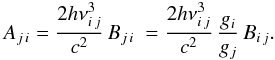
The corresponding oscillator strength fij is obtained from the relation
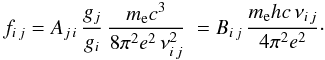
The computationally most expensive part of solving the non-LTE problem is the calculation of the line-blanketed radiation field Jν(x,y,z,t) at each grid point of the selected 3D models, which is needed to determine the photoionization rates for all atomic levels. This is done with a modified version of the radiation transport routines that are used in the CO5BOLD hydrodynamical simulations for computing the radiative energy exchange term ∇Frad(x,y,z). The solution of the radiative transfer equation is based on a Feautrier scheme applied to a set of long characteristics. The continuous opacities used in this context are computed with the routines IONDIS & OPALAM from the Kiel stellar atmosphere package10. Line blanketing is taken into account by adding to the continuous opacity the opacity distribution functions (ODFs, “big division”, vturb = 2 km s-1) of Castelli & Kurucz (2003), including the H i - H + and H i-H i quasi-molecular absorption near 1400 and 1600 Å, respectively. There is a slight inconsistency in the chemical composition adopted for the calculation of the opacities: the continuous opacities are based on the solar abundances of Asplund et al. (2005), while the ODFs rely on the solar composition of Grevesse & Sauval (1998). To obtain the opacities for different metallicities, the solar abundances were scaled by a global factor corresponding to the desired [M/H], with an enhancement of the α-elements by 0.4 dex below [M/H] = −0.5. A total of 600 frequency points were used to obtain the Jν between λ 925 and 19800 Å. We checked that treating continuous scattering as true absorption does not introduce any significant changes in the resulting departure coefficients.
Energy levels of the Li i model atom.
Bound-bound transitions of the Li i model atom.
Given the line-blanketed radiation field Jν(x,y,z,t), the photoionization rate Piκ from level i to the continuum κ is computed as
![\appendix \setcounter{section}{1} \begin{equation} P_{i\,\kappa}~= 4\,\pi\,\int_{{\nu}_i}^\infty \frac{\alpha_i(\nu)\,J_\nu}{h\nu}\, \mathrm{d}\nu\, \quad [{\rm s}^{-1}], \end{equation}](/articles/aa/full_html/2010/14/aa13282-09/aa13282-09-eq179.png)
where νi is the threshold photoionization frequency for level i, and the photoionization cross-sections αi(ν) for all considered atomic levels are taken from the TOPBASE Opacity Project on-line atomic database at the “Centre de données astronomiques de Strasbourg”11. The photo-recombination rates Pκi from the continuum κ to level i are then given by
![\appendix \setcounter{section}{1} \begin{eqnarray} P_{\kappa\,i} &=& 4\,\pi\,\int_{{\nu}_i}^\infty \frac{\alpha_i(\nu)\,B_\nu(T)}{h\nu}\, \left(1-\exp\left\{-\frac{h\nu}{kT}\right\}\right)\,{\rm d}\nu \nonumber \\ &&+ 4\,\pi\,\int_{{\nu}_i}^\infty \frac{\alpha_i(\nu)\,J_\nu}{h\nu}\, \exp\left\{-\frac{h\nu}{kT}\right\}\,\mathrm{d}\nu\, \quad [{\rm s}^{-1}], \end{eqnarray}](/articles/aa/full_html/2010/14/aa13282-09/aa13282-09-eq183.png)
Bν(T) denoting the Kirchhoff-Planck function at local temperature T and frequency ν.
Cross-sections for the collisional ionization and excitation by electrons are computed according to the prescriptions of Seaton (1962) and Van Regemorter (1962), respectively, as given by Allen (1976) and Cox (2000). The oscillator strengths fij from Table A.2 are needed to calculate the collisional excitation cross-sections. Collisional ionization by neutral hydrogen via the charge transfer reaction H(1s) + Li(nl) → Li+(1s2) + H−, and the reverse process H− + Li+(1s2) → H(1s) + Li(nl), are treated according to Barklem et al. (2003) for the first 7 levels. Collisional excitation by neutral hydrogen is ignored, as it was found to be unimportant for thermalizing Li i by Barklem et al. (2003).
The departure coefficients
bi(x,y,z) are finally
obtained by solving the statistical equilibrium equations locally at each grid point
(x,y,z). The profile-averaged radiation field at the line transitions,
 , determines the radiative excitation rates
![\appendix \setcounter{section}{1} \begin{equation} R_{i\,j}= B_{i\,j}\, \overline{J}(\nu_{i\,j}) \equiv B_{i\,j}\,\int_{{\rm line}\; i\,j} \phi_\nu\,J_\nu\, \mathrm{d}\nu\, \quad [{\rm s}^{-1}], \end{equation}](/articles/aa/full_html/2010/14/aa13282-09/aa13282-09-eq193.png)
and the radiative de-excitation rates
![\appendix \setcounter{section}{1} \begin{equation} R_{j\,i}=\frac{g_j}{g_i}\,B_{j\,i}\,\left(\frac{2h\nu_{i\,j}^3}{c^2} + \overline{J}(\nu_{i\,j})\right)\, \quad [{\rm s}^{-1}], \end{equation}](/articles/aa/full_html/2010/14/aa13282-09/aa13282-09-eq194.png)
where the statistical
weights of lower and upper level, gi and
gj, and the Einstein coefficients
Bij are taken from Table A.2. For the line profile
φν we assume a purely Gaussian
distribution (identical for absorption and emission) with a line width that corresponds to
the local thermal Doppler velocity plus a microturbulence of 1.5 km s-1. The
Doppler shift caused by the line-of-sight component of the hydrodynamical velocity field
is ignored in the present computation. For all transitions except for the resonance line,
was replaced by the mean continuum intensity
Jν. For the resonance line (transition #1),
the line opacity was taken into account for the computation of , assuming an f-value of 0.48975
(about 2/3 of the value given in Table A.2 to
represent only the main component of the doublet), together with a typical lithium
abundance of A(Li) = 2.2.
Since is a non-local quantity that depends in turn on
the bi, a Λ-iteration is employed to obtain a
consistent solution. Fortunately, the Λ iteration converges very rapidly, because even the
Li i resonance line affects the radiation field only marginally, while all the
other lines are very weak. Typically, three iterations are sufficient to achieve
convergence.
Finally, the departure coefficients bi are used in the line formation code Linfor3D to compute the non-LTE line opacity
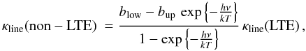
and the line source function
where blow and bup are the departure coefficients of lower and upper level, respectively, and Bν is again the Kirchhoff-Planck function.
Appendix B: Analytical fit to 3D NLTE Li abundance as a function of stellar parameters and EW
B.1. Introduction
It is often convenient to have tabular data on an irregular grid y = y(x) condensed into a single function (even with many fit parameters), instead of having to interpolate between the original data points. Choosing a fitting function that is linear in all parameters (e.g., a sum of polynomials as A + Bx + Cx2 or sine/cosine functions) results in a comparatively simple linear problem for finding these parameters, usually with one unique solution. However, the result might not have the desired extrapolation behavior, might be “too wiggly” between the data points, or produce no good fit at all.
A more effective approach might then be to start with a properly crafted function, possibly non-linear, and having fitting parameters “within” the terms as in Aexp(B + Cx). In this case, an iterative process is necessary to determine these parameters. This iteration requires starting values, which will affect the convergence of the process and also the solution if one is found: in this case, the scheme might diverge or converge to different local minima, depending on the starting point. However, this last issue is hardly a problem for our application – we are content with a good fit, and do not necessarily need to achieve the closest one. We continue, however, to have the problem of constructing the fitting function and choosing the initial values for the parameters.
B.2. Method
We used a scheme for recursive term substitution, written in IDL, that attempted not only to find optimum fitting parameters for a given function, but also to automatically determine the optimum functional form itself. The latter was chosen from a set of candidates given by a list of terms and some construction rules. The usual starting point was a constant “function” with one parameter, say A, the best “fit” for which is the mean of y. In each recursion step, all parameters were successively substituted with all of the terms from a list (with possible restrictions), for instance
or
The initial values of (A0, A1, A2) were derived from A by e.g., assuming A0 = A,A1 = 0.1 × A,A2 = 0. Applying a modified version of the IDL function curvefit (requiring also partial derivatives) provided the optimum parameter set for the given function and start values.
This process was repeated with a number of random variations to approach an optimum solution for the given function. The final solution was the globally best fit among all candidate functions and parameters.
The main control parameters are the list of candidate terms and the recursion depth. For the current application, we search a 4D function

where (x0,x1,x2,x3) = (log (EW), log Teff, log g, [Fe/H]), or, for the inverse problem, (A(Li), log Teff, log g, [Fe/H]). We start with
![\appendix \setcounter{section}{2} \begin{displaymath} A_0 + \log_{10}[1 - \exp(- 10^{(X_0-A_1)})] \end{displaymath}](/articles/aa/full_html/2010/14/aa13282-09/aa13282-09-eq223.png)
to determine the equivalent width as a function of abundance, based on a simple absorption model for a box-shaped line profile. In the following recursion steps, we replace the parameters with linear terms

which finally results in higher-order polynomials instead of the initial coefficients. In this step, the variation in the COG with the stellar parameters is taken into account. In the process of applying the term substitution, we scanned through several hundred possible functional forms. We decided the most suitable one on the basis of simplicity, and its ability to represent the numerical data with sufficient accuracy.
As described in Sect. 6.1, synthetic grids were computed for three cases, 3D NLTE, 1D LHD NLTE, and 1D LHD LTE. This in principle leads to 6 fitting functions being computed, when both the EW → A(Li) and A(Li) → EW forms are required. We decided to force all three functions in either sense to have the same form, differing only by their parameters. We thus first searched an optimum function for one case (A(Li) → 1D LHD NLTE turned out to be the optimum choice) and then varied only the parameters (and not the functional form) for the other two cases. The final inversion of the function was performed by hand.
B.3. Best-fitting functions
Best-fitting functional forms were produced both to derive A(Li) from EW and to derive EW from A(Li), the latter being useful, e.g., for the preparation of observations. Analytical fit formulae for both cases are presented in Eq. (B.1); fitting coefficients are listed in Table B.1. Three sets of coefficients are listed. The 3D NLTE set is used to fit computations where CO5BOLD 3D hydrodynamical models are used in association with a 3D NLTE time-dependent spectrosynthesis. The 1D NLTE and LTE cases refer instead to computations performed by using LHD one-dimensional models, with spectrosynthesis performed with or
without the inclusion of NLTE effects, based on the same physics and model atoms as for the 3D NLTE case:
![\appendix \setcounter{section}{2} \begin{eqnarray} % \label{fitform}&&\!\!\!\!\!\! Q_1 = A_8 + A_{11}\log T_{\rm eff} + A_{12} \log g + A_{13} {\rm [Fe/H]} \nonumber \\ &&\!\!\!\!\!\! Q_2 = A_6 + Q_1 \log T_{\rm eff} +A_9 \log g + A_{10} {\rm [Fe/H]} \nonumber \\ &&\!\!\!\!\!\! Q_3 = A_2 + A_5 \log T_{\rm eff} + Q_2 \log g + A_7 {\rm [Fe/H]} \nonumber \\ &&\!\!\!\!\!\! Q_4 = A_1+Q_3 \log T_{\rm eff} +A_3 \log g + A_4 {\rm [Fe/H]}\nonumber \\[0.5mm] &&\!\!\!\!\!\! A({\rm Li}) ~= A_1 + Q_3 \log T_{\rm eff} + A_3 \log g + A_4 {\rm [Fe/H]}\nonumber \\ &&\!\!\!\!\!\! ~~~~~~~~~~~~ +\log[-\ln(1-EW 10^{-A_0}) ]\nonumber \\[0.5mm] &&\!\!\!\!\!\! \log\,EW = A_0 + \log [ ~| 1 + \exp (-10^{A(Li)-Q_4})|~ ]. % \end{eqnarray}](/articles/aa/full_html/2010/14/aa13282-09/aa13282-09-eq229.png)
Units are expected to be K for temperature, cm s-2 for log g, and mÅ for EW. As for any fit, extrapolation reliability is difficult to assess. Owing to the high computational cost of 3D-atmosphere model calculations, we limited our grid to the currently available models, which obliged us to extrapolate towards high gravities by 0.4 dex and towards low metallicities by about 0.6 dex. Both extrapolations should be quite safe, since the 670.8 nm Li doublet should be quite insensitive to both parameters. Because of the vanishing line opacity, atmosphere models are scarcely sensitive to metallicity variations below [Fe/H] = −3. Those who might wish to employ the presented formulae to derive Li abundances are nevertheless advised to use caution when extrapolating, especially in Teff and EW. In particular, the saturation part of the COG is almost unsampled, and one cannot expect the present fit to reproduce it properly. Fitting to EW significantly above 100 pm is therefore not advisable.
Coefficients for the analytical fit of EW → A(Li) and A(Li) → EW.
Grid available at http://wwwuser.oat.ts.astro.it/castelli/
The original version is available online at http://kurucz.harvard.edu/
The corresponding IDL functions are also available on-line at http://mygepi.obspm.fr/~sbordone/fitting.html or by email request to the authors.
Delaunay triangulation is a method of triangulation of a set P of points in a plane defined as the triangulation for which no element of P lies within the circumcircle of each triangle, except for the triangle vertexes. It is often used to model surfaces that are sampled on irregular grids (e.g., elevations in geography). The built-in IDL functions triangulate and trigrid have been used to produce the triangulation and the interpolation based on it.
We have another UVES spectrum of CS 22188–033, taken at a different epoch, which does not show radial velocity variations with respect to the one used in the present work, nor signs of a double line system.
González Hernández et al. (2008) derived Teff from photometry and isochrones, but a cross-check with Hα profiles computed in 1D with Barklem et al. (2000a) broadening confirmed the result.
Acknowledgments
Authors L.S., P.B., H.-G.L., N.B., and J.G.-H. acknowledge financial support from EU contract MEXT-CT-2004-014265 (CIFIST). We acknowledge use of the supercomputing center CINECA, which has granted us time to compute part of the hydrodynamical models used in this investigation, through the INAF-CINECA agreement 2006, 2007. T.C.B. acknowledges partial support for this work from grant 08-22648: Physics Frontier Center/Joint Institute for Nuclear Astrophysics. This research has made use of the SIMBAD database, operated at CDS, Strasbourg, France, and of NASA’s Astrophysics Data System. This publication makes use of data products from the Two Micron All Sky Survey, which is a joint project of the University of Massachusetts and the Infrared Processing and Analysis Center/California Institute of Technology, funded by the National Aeronautics and Space Administration and the National Science Foundation. We also wish to thank K. Lind for making available to us her code to interpolate the NLTE correction tables of Lind et al. (2009a).
References
- Ali, A. W., & Griem, H. R. 1966, Phys. Rev., 144, 366 [NASA ADS] [CrossRef] [Google Scholar]
- Allard, N. F., Kielkopf, J. F., Cayrel, R., & van’t Veer-Menneret, C. 2008, A&A, 480, 581 [NASA ADS] [CrossRef] [EDP Sciences] [Google Scholar]
- Allen, C.W. 1976, Astrophysical Quantities, 3rd edition (The Athlone Press), 41 [Google Scholar]
- Alonso, A., Salaris, M., Arribas, S., Martínez-Roger, C., & AsensioRamos, A. 2000, A&A, 355, 1060 [NASA ADS] [Google Scholar]
- Alonso, A., Arribas, S., & Martínez-Roger, C. 2001, A&A, 376, 1039 [NASA ADS] [CrossRef] [EDP Sciences] [Google Scholar]
- Alvarez, R., & Plez, B. 1998, A&A, 330, 1109 [NASA ADS] [Google Scholar]
- Aoki, W., Barklem, P. S., Beers, T. C., et al. 2009, ApJ, 698, 1803 [NASA ADS] [CrossRef] [Google Scholar]
- Asplund, M., Gustafsson, B., Kiselman, D., & Eriksson, K. 1997, A&A, 318, 521 [NASA ADS] [Google Scholar]
- Asplund, M., Grevesse, N., & Sauval, A. J. 2005, Cosmic Abundances as Records of Stellar Evolution and Nucleosynthesis, ASP Conf. Ser., 336, 25 [Google Scholar]
- Asplund, M., Lambert, D. L., Nissen, P. E., Primas, F., & Smith, V. V. 2006, ApJ, 644, 229 [NASA ADS] [CrossRef] [Google Scholar]
- Barklem, P. S., Piskunov, N., & O’Mara, B. J. 2000a, A&A, 355, L5 [NASA ADS] [Google Scholar]
- Barklem, P. S., Piskunov, N., & O’Mara, B. J. 2000b, A&A, 363, 1091 [NASA ADS] [Google Scholar]
- Barklem, P. S., Stempels, H. C., Allen de Prieto, C., et al. 2002, A&A, 385, 951 [NASA ADS] [CrossRef] [EDP Sciences] [Google Scholar]
- Barklem, P. S., Belyaev, A. K., & Asplund, M. 2003, A&A, 409, L1 [NASA ADS] [CrossRef] [EDP Sciences] [Google Scholar]
- Barklem, P. S., Christlieb, N., Beers, T. C., et al. 2005, A&A, 439, 129 [NASA ADS] [CrossRef] [EDP Sciences] [Google Scholar]
- Beers, T. C. 1999, Ap&SS, 265, 547 [NASA ADS] [CrossRef] [Google Scholar]
- Beers, T. C., Preston, G. W., & Shectman, S. A. 1985, AJ, 90, 2089 [NASA ADS] [CrossRef] [Google Scholar]
- Beers, T. C., Preston, G. W., & Shectman, S. A. 1992, AJ, 103, 1987 [NASA ADS] [CrossRef] [Google Scholar]
- Behara, N. T., Ludwig, H.-G., Steffen, M., & Bonifacio, P. 2009, AIP Conf. Ser., 1094, 784 [NASA ADS] [CrossRef] [Google Scholar]
- Blackwell, D. E., & Shallis, M. J. 1977, MNRAS, 180, 177 [NASA ADS] [CrossRef] [Google Scholar]
- Blackwell, D. E., Petford, A. D., & Shallis, M. J. 1980, A&A, 82, 249 [NASA ADS] [Google Scholar]
- Blackwell, D. E., Petford, A. D., Arribas, S., Haddock, D. J., & Selby, M. J. 1990, A&A, 232, 396 [NASA ADS] [Google Scholar]
- Boesgaard, A. M., Stephens, A., & Deliyannis, C. P. 2005, ApJ, 633, 398 [NASA ADS] [CrossRef] [Google Scholar]
- Bonifacio, P., & Molaro, P. 1997, MNRAS, 285, 847 [NASA ADS] [CrossRef] [Google Scholar]
- Bonifacio, P., Monai, S., & Beers, T. C. 2000, AJ, 120, 2065 [NASA ADS] [CrossRef] [Google Scholar]
- Bonifacio, P., Molaro, P., Sivarani, T., et al. 2007, A&A, 462, 851 [NASA ADS] [CrossRef] [EDP Sciences] [Google Scholar]
- Caffau, E., & Ludwig, H.-G. 2007, A&A, 467, L11 [NASA ADS] [CrossRef] [EDP Sciences] [Google Scholar]
- Caffau, E., Steffen, M., Sbordone, L., Ludwig, H.-G., & Bonifacio, P. 2007, A&A, 473, L9 [NASA ADS] [CrossRef] [EDP Sciences] [Google Scholar]
- Carretta, E., Gratton, R., Cohen, J. G., Beers, T. C., & Christlieb, N. 2002, AJ, 124, 481 [NASA ADS] [CrossRef] [Google Scholar]
- Carlsson, M., Rutten, R. J., Bruls, J. H. M. J., & Shchukina, N. G. 1994, A&A, 288, 860 [NASA ADS] [Google Scholar]
- Castelli, F., & Kurucz, R. L. 2003, Modelling of Stellar Atmospheres, 210, 20P, [arXiv:astro-ph/0405087] [Google Scholar]
- Cayrel, R. 1988, in The Impact of Very High S/N Spectroscopy on Stellar Physics, ed. G. Cayrel de Strobel, & M. Spite (Dordrecht: Kluwer), 345 [Google Scholar]
- Cayrel, R., Steffen, M., Chand, H., et al. 2007, A&A, 473, L37 [NASA ADS] [CrossRef] [EDP Sciences] [Google Scholar]
- Charbonnel, C., & Primas, F. 2005, A&A, 442, 961 [NASA ADS] [CrossRef] [EDP Sciences] [Google Scholar]
- Christlieb, N., Schörck, T., Frebel, A., et al. 2008, A&A, 484, 721 [NASA ADS] [CrossRef] [EDP Sciences] [Google Scholar]
- Cohen, J. G., Christlieb, N., Beers, T. C., Gratton, R., & Carretta, E. 2002, AJ, 124, 470 [NASA ADS] [CrossRef] [Google Scholar]
- Cox, A. N. 2000, Allen’s Astrophysical Quantities, 4rd edition, ed. A. N. Cox, AIP (Springer), 40 [Google Scholar]
- Cyburt, R. H., Fields, B. D., & Olive, K. A. 2008, J. Cosmol. Astro-Part. Phys., 11, 12 [Google Scholar]
- Dekker, H., D’Odorico, S., Kaufer, A., Delabre, B., & Kotzlowski, H. 2000, Proc. SPIE, 4008, 534 [Google Scholar]
- Dunkley, J., Komatsu, E., Nolta, M. R., et al. 2009, ApJS, 180, 306 [NASA ADS] [CrossRef] [Google Scholar]
- Duquennoy, A., Mayor, M., & Halbwachs, J.-L. 1991, A&AS, 88, 281 [Google Scholar]
- Edvardsson, B., Andersen, J., Gustafsson, B., et al. 1993, A&A, 275, 101 [NASA ADS] [Google Scholar]
- Frebel, A., Collet, R., Eriksson, K., Christlieb, N., & Aoki, W. 2008, ApJ, 684, 588 [NASA ADS] [CrossRef] [Google Scholar]
- Freytag, B., Steffen, M., & Dorch, B. 2002, Astron. Nachr., 323, 213 [NASA ADS] [CrossRef] [EDP Sciences] [Google Scholar]
- Fuhrmann, K., Axer, M., & Gehren, T. 1993, A&A, 271, 451 [NASA ADS] [Google Scholar]
- García Pérez, A. E., Christlieb, N., Ryan, S. G., et al. 2008, Physica Scripta V. T, 133, 014036 [NASA ADS] [CrossRef] [Google Scholar]
- González Hernández, J. I., & Bonifacio, P. 2009, A&A, 497, 497 [NASA ADS] [CrossRef] [EDP Sciences] [Google Scholar]
- González Hernández, J. I., Bonifacio, P., Ludwig, H.-G., et al. 2008, A&A, 480, 233 [NASA ADS] [CrossRef] [EDP Sciences] [MathSciNet] [Google Scholar]
- Grevesse, N., & Sauval, A. J. 1998, Space Sci. Rev., 85, 161 [NASA ADS] [CrossRef] [Google Scholar]
- Gustafsson, B., Bell, R. A., Eriksson, K., & Nordlund, A. 1975, A&A, 42, 407 [NASA ADS] [Google Scholar]
- Gustafsson, B., Edvardsson, B., Eriksson, K., et al. 2003, Stellar Atmosphere Modeling, 288, 331 [NASA ADS] [Google Scholar]
- Hosford, A., Ryan, S. G., García Pérez, A. E., Norris, J. E., & Olive, K. A. 2009, A&A, 493, 601 [NASA ADS] [CrossRef] [EDP Sciences] [Google Scholar]
- Iocco, F., Mangano, G., Miele, G., Pisanti, O., & Serpico, P. D. 2009, Phys. Rep., 472, 1 [NASA ADS] [CrossRef] [Google Scholar]
- Kippenhahn, R., & Weigert, A. 1990, Stellar Structure and Evolution (Berlin, Heidelberg, New York: Springer-Verlag), XVI, 468, also Astronomy and Astrophysics Library [Google Scholar]
- Komiya, Y., Suda, T., & Fujimoto, M. Y. 2009, ApJ, 694, 1577 [NASA ADS] [CrossRef] [Google Scholar]
- Korn, A. J., Grundahl, F., Richard, O., et al. 2006, Nature, 442, 657 [Google Scholar]
- Korn, A. J., Grundahl, F., Richard, O., et al. 2007, ApJ, 671, 402 [NASA ADS] [CrossRef] [Google Scholar]
- Kurucz, R. L. 2005, Mem. Soc. Astron. Ital. Suppl., 8, 14 [Google Scholar]
- Latham, D. W., Stefanik, R. P., Torres, G., et al. 2002, AJ, 124, 1144 [NASA ADS] [CrossRef] [Google Scholar]
- Lind, K., Asplund, M., & Barklem, P. S. 2009a, A&A, 503, 541 [NASA ADS] [CrossRef] [EDP Sciences] [Google Scholar]
- Lind, K., Primas, F., Charbonnel, C., Grundahl, F., & Asplund, M. 2009b, A&A, 503, 545 [NASA ADS] [CrossRef] [EDP Sciences] [MathSciNet] [Google Scholar]
- Ludwig, H.-G., Behara, N. T., Steffen, M., & Bonifacio, P. 2009a, A&A, 502, L1 [NASA ADS] [CrossRef] [EDP Sciences] [MathSciNet] [Google Scholar]
- Ludwig, H.-G., Caffau, E., Steffen, M., et al. 2009b, Mem. Soc. Astron. Ital., 80, 711 [Google Scholar]
- Meléndez, J., & Ramírez, I. 2004, ApJ, 615, L33 [NASA ADS] [CrossRef] [Google Scholar]
- Michaud, G., Fontaine, G., & Beaudet, G. 1984, ApJ, 282, 206 [NASA ADS] [CrossRef] [Google Scholar]
- Molaro, P. 2008, Pathways Through an Eclectic Universe, 390, 472 [NASA ADS] [Google Scholar]
- Pettini, M., Zych, B. J., Murphy, M. T., Lewis, A., & Steidel, C. C. 2008, MNRAS, 391, 1499 [NASA ADS] [CrossRef] [MathSciNet] [Google Scholar]
- Piau, L. 2008, ApJ, 689, 1279 [NASA ADS] [CrossRef] [Google Scholar]
- Piau, L., Beers, T. C., Balsara, D. S., et al. 2006, ApJ, 653, 300 [NASA ADS] [CrossRef] [Google Scholar]
- Plez, B., Brett, J. M., & Nordlund, A. 1992, A&A, 256, 551 [NASA ADS] [Google Scholar]
- Press, W. H., Teukolsky, S. A., Vetterling, W. T., & Flannery, B. P. 1992 (Cambridge: University Press), 2nd ed. [Google Scholar]
- Richard, O., Michaud, G., & Richer, J. 2005, ApJ, 619, 538 [NASA ADS] [CrossRef] [Google Scholar]
- Ryan, S. G., Beers, T. C., Deliyannis, C. P., & Thorburn, J. A. 1996, ApJ, 458, 543 [NASA ADS] [CrossRef] [Google Scholar]
- Ryan, S. G., Norris, J. E., & Beers, T. C. 1999, ApJ, 523, 654 [NASA ADS] [CrossRef] [Google Scholar]
- Sbordone, L. 2005, Mem. Soc. Astron. Ital. Suppl., 8, 61 [Google Scholar]
- Sbordone, L., Bonifacio, P., Castelli, F., & Kurucz, R. L. 2004, Mem. Soc. Astron. Ital. Suppl., 5, 93 [Google Scholar]
- Schlegel, D. J., Finkbeiner, D. P., & Davis, M. 1998, ApJ, 500, 525 [NASA ADS] [CrossRef] [Google Scholar]
- Seaton, M.J. 1962, in Atomic and Molecular Processes, ed. D.R. Bates, 375 [Google Scholar]
- Skrutskie, M. F., Cutri, R. M., Stiening, R., et al. 2006, AJ, 131, 1163 [NASA ADS] [CrossRef] [Google Scholar]
- Spite, M., & Spite, F. 1982a, Nature, 297, 483 [NASA ADS] [CrossRef] [Google Scholar]
- Spite, F., & Spite, M. 1982b, A&A, 115, 357 [NASA ADS] [Google Scholar]
- Stehlé, C., & Hutcheon, R. 1999, A&AS, 140, 93 [NASA ADS] [CrossRef] [EDP Sciences] [Google Scholar]
- Steigman, G. 2001, [arXiv:astro-ph/0107222] [Google Scholar]
- Steigman, G. 2007, Ann. Rev. Nucl. Particle Science, 57, 463 [Google Scholar]
- Steigman, G. 2009, AIPC, 1135, 94 [NASA ADS] [Google Scholar]
- Tolstoy, E., Hill, V., & Tosi, M. 2009, ARA&A, 47, 371 [NASA ADS] [CrossRef] [Google Scholar]
- Van Regemorter, H. 1962, ApJ, 136, 906 [NASA ADS] [CrossRef] [Google Scholar]
- van’t Veer-Menneret, C., & Megessier, C. 1996, A&A, 309, 879 [NASA ADS] [Google Scholar]
- Venn, K. A., & Lambert, D. L. 2008, ApJ, 677, 572 [NASA ADS] [CrossRef] [Google Scholar]
- Wagoner, R. V., Fowler, W. A., & Hoyle, F. 1967, ApJ, 148, 3 [NASA ADS] [CrossRef] [Google Scholar]
- Wedemeyer, S., Freytag, B., Steffen, M., Ludwig, H.-G., & Holweger, H. 2004, A&A, 414, 1121 [NASA ADS] [CrossRef] [EDP Sciences] [Google Scholar]
All Tables
Atmosphere parameters for the program stars using the different temperature estimators.
Fe i and Fe ii mean abundances, as well as their associated σ for the four temperature scales.
Li i 670.8 nm EW and errors, and lithium abundances using the different parameter sets.
Parameters of the models in the 3D CO5BOLD and 1D LHD grids used in the 3D NLTE Li abundances, and in the computation of NLTE corrections.
Barycentric radial velocities for the two components of the binary system HE1148–0037 as measured from the spectra available to us.
All Figures
|
Fig. 1 High-resolution spectra of the Li i 670.79 nm doublet region for the 11 newly observed stars of the sample. For stars for which multiple spectra were available, the coadded spectrum is shown. For the purpose of visualization, all the spectra have been shifted to zero radial velocity and normalized. Teff increases from bottom to top, 3D scale Teff and A(Li)3D,NLTE (see Sects. 4 and 6) are listed for each star. The star CS 22882–027 shows no detectable Li line, and the 3σ upper limit to A(Li) is listed here. |
| In the text | |
|
Fig. 2 Hα red wing profiles in the wavelength range significant for the fit. In each panel, red profiles (upper ones) are for Teff = 5400 K, black profiles (middle ones) are for Teff = 6000 K, and blue profiles (lower) for Teff = 6600 K. For each temperature, dashed profiles are for log g = 3.5, solid profiles for log g = 4.0, and dotted profiles are for log g = 4.5. All profiles assume [Fe/H] = −3. Upper panel shows profiles for BA temperatures, lower panel for ALI temperatures. |
| In the text | |
|
Fig. 3 Hα theoretical profiles for models with log g = 4, [Fe/H] = −3 (solid lines) and log g = 4, [Fe/H] = −2.5 (dot-dashed lines) have been fitted with the same procedure used for the program stars, but using a log g = 3.5 grid (red lines with filled circles) and a log g = 4.5 grid (blue lines with open diamonds). Here we plot the temperature difference (Teff(log g = 3.5/4.5) – Teff(log g = 4.0)), against the “real” effective temperature of the profile. The upper panel shows BA profiles, the middle panel ALI profiles, and lower panel 3D profiles. The gray shaded areas indicates the temperature ranges for the program stars in each Teff scale. |
| In the text | |
|
Fig. 4 Effective temperatures for different estimators, plotted against BA temperature for the program stars. Top to bottom: ALI, IRFM and 3D temperatures. The red line represents the one-to-one relation (hence the line of BA temperatures). |
| In the text | |
|
Fig. 5 Effective temperatures for different estimators, plotted against [Fe/H] (as derived using the temperature in the panel). Top to bottom: BA temperatures, then ALI, IRFM and 3D. |
| In the text | |
|
Fig. 6 Difference between A(Li)f and A(Li)i plotted against Teff and the Li doublet EW. The two “outliers” are labeled. |
| In the text | |
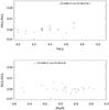 |
Fig. 7 Same as in Fig. 6 but now plotting against log g and [Fe/H]. |
| In the text | |
|
Fig. 8 The NLTE correction (A(Li)1D,NLTE – A(Li) 1D,LTE), computed for each star using our model atom (black filled dots) along with the Carlsson et al. (1994) values (red open circles), plotted against Teff and log g. The 3D temperature scale is assumed. |
| In the text | |
|
Fig. 9 The NLTE correction (A(Li)1D,NLTE – A(Li) 1D,LTE), computed for each star using our model atom (black filled dots) along with the Lind et al. (2009a) values (red open circles), plotted against Teff and log g. The 3D temperature scale is assumed, and [Fe/H] = −3 is imposed for all stars. |
| In the text | |
|
Fig. 10 Li abundance versus [Fe/H] for the four temperature estimates. Top to bottom, BA, ALI, IRFM, and 3D temperatures. For the 3D temperature scale, the black triangles represent the 3D NLTE Li abundances, while the red crosses represent 1D LTE Li abundances with the NLTE corrections applied. The best-fit linear relation (as per Table 8) is indicated by a gray line. A typical error bar of ± 0.09 dex in Li abundance and the average [Fe/H] error bar are also displayed. |
| In the text | |
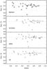 |
Fig. 11 Residuals of the best fit of A(Li) vs. [Fe/H] listed in Table 8. |
| In the text | |
|
Fig. 12 Li abundance versus effective temperature for the four temperature estimates. Symbols are the same as in Fig. 10. Typical error bars of ± 0.09 dex in the Li abundance and ± 130 K in Teff are also displayed. The best-fit linear relation as per Table 8 is indicated by a gray line. |
| In the text | |
|
Fig. 13 The Mg i 517.268 nm line for HE 1148–0037, in spectra taken at JD 2 453 787.6803 (black continuous line) and JD 2 453 823.5443 (red dashed line), separated by 35.86 days. The spectra have been normalized, and Doppler shifted to bring the primary component to a rest-frame wavelength. The binarity is readily visible, as well as the variation in the components’ separation. |
| In the text | |
|
Fig. 14 Comparison between the results of this work and of Bonifacio et al. (2007) for the 17 stars in common. In the upper panel, the difference between our Teff and the Bonifacio et al. (2007)Teff determination is plotted against the value of log g in Bonifacio et al. (2007). In the center panel, we show [Fe/H] difference, and in the lower panel, the difference in the A(Li) LTE. For our results, BA temperature scale is used. |
| In the text | |
|
Fig. 15 A unified view of A(Li) vs. [Fe/H] from some studies for which a common temperature scale can be assumed. Blue circles, Asplund et al. (2006) data, red triangles, Aoki et al. (2009) data, magenta squares, CS 22876–032 from González Hernández et al. (2008), filled symbol primary star, open symbol secondary star. Black diamonds, this work, BA temperature scale. Dot-dashed gray line, best linear fit to Asplund et al. (2006) data, continuous dark gray line, best fit to our data. Typical error bars for our data are displayed. |
| In the text | |
Current usage metrics show cumulative count of Article Views (full-text article views including HTML views, PDF and ePub downloads, according to the available data) and Abstracts Views on Vision4Press platform.
Data correspond to usage on the plateform after 2015. The current usage metrics is available 48-96 hours after online publication and is updated daily on week days.
Initial download of the metrics may take a while.