| Issue |
A&A
Volume 522, November 2010
|
|
|---|---|---|
| Article Number | A68 | |
| Number of page(s) | 15 | |
| Section | Catalogs and data | |
| DOI | https://doi.org/10.1051/0004-6361/200912216 | |
| Published online | 04 November 2010 | |
The catalog of variable sources detected by INTEGRAL
I. Catalog and techniques*
1
DESY Zeuthen,
Platanenallee 6,
15738
Zeuthen,
Germany
e-mail: This email address is being protected from spambots. You need JavaScript enabled to view it.
2
Astronomical Observatory of Kiev University,
Observatorna 3,
04058
Kiev,
Ukraine
3
INAF/IASF Milano,
via E. Bassini 15, 20133
Milano,
Italy
4
ISDC Data Centre for Astrophysics,
Chemin d’Écogia 16,
1290
Versoix,
Switzerland
5
Observatoire Astronomique de l’Université de Genève,
Chemin des Maillettes
51, 1290
Sauverny,
Switzerland
Received:
27
March
2009
Accepted:
27
April
2010
Abstract
Context. During its 6 years of operation, INTEGRAL/ISGRI has detected more than 500 sources. Many of these sources are variable. Taking into account that nearly half of INTEGRAL/ISGRI sources are new and many of them remain unidentified, the variability properties of the sources can provide additional constraints to help us to classify and identify the unknown sources.
Aims. To study the variability properties of the sources detected by INTEGRAL/ISGRI, we develop a method to quantify the variability of a source. We describe here our techniques and compile a catalog of the sources that fit our criteria of variability.
Methods. We use the natural time binning of INTEGRAL observations called Science Window (≈2000 s) and test the hypothesis that the detected sources are constant using a χ2 all-sky map in three energy bands (20–40, 40–100, 100–200 keV). We calculate an intrinsic variance of the flux in individual pixels and use it to define the fractional variability of a source. The method is sensitive to the source variability on timescales of one Science Window and higher. We concentrate only on the sources that were already reported to be detected by INTEGRAL.
Results. We present a catalog of 202 sources found to be significantly variable. For the catalog sources, we give the measure of variability and fluxes with corresponding errors in the 20–40, 40–100 and 100–200 keV energy bands, and we present some statistics about the population of variable sources. The description of the physical properties of the variable sources will be given in a forthcoming paper.
Key words: gamma-rays: observations / catalogs
Table 3 is also available in electronic form at the CDS via anonymous ftp to cdsarc.u-strasbg.fr (130.79.128.5) or via http://cdsarc.u-strasbg.fr/viz-bin/qcat?J/A+A/522/A68
© ESO, 2010
1. Introduction
INTEGRAL (INTErnational Gamma Ray Astrophysics Laboratory, Winkler et al. (2003)) was launched in 2002 and since then has performed high-quality observations in the energy band from 3 keV up to ~10 MeV. The INTEGRAL payload consists of two main soft gamma-ray instruments (the imager IBIS Ubertini et al. 2003, and the spectrometer SPI Vedrenne et al. 2003) and two monitors (in X-rays JEM-X Lund et al. 2003, and in optical OMC Mas-Hesse et al. 2003). The wide field-of-view of the imager IBIS provides an ideal opportunity to survey the sky in hard X-rays.
During its first 6 years in orbit, INTEGRAL has covered nearly the whole sky. The observational data have been mainly used to study the soft gamma-ray emission from the Galactic plane (GP) (Bouchet et al. 2005; Krivonos et al. 2007) through the Galactic plane scans and the Galactic centre (GC) Bélanger et al. (2004)Revnivtsev et al. (2004)Bélanger et al. (2006)Krivonos et al. (2007) through the Galactic centre deep exposure programme. A number of papers have already presented general surveys (Bazzano et al. 2006; Bird et al. 2007) of the sky as well as of specific regions (Götz et al. 2006; den Hartog et al. 2006; Molkov et al. 2004) and population types (Barlow et al. 2006; Bassani et al. 2007; Sazonov et al. 2007; Beckmann et al. 2006, 2009).
The majority of the classified sources detected by INTEGRAL are either low and high mass X-ray binaries (LMXBs and HMXBs) or AGNs (Bodaghee et al. 2007). However, a significant fraction of the detected sources remain unidentified. A special approach to population classification is required for the GC region to resolve the population types because of the high density of sources. Fortunately, the physics of the sources may help us to unveil their type. Indeed, the bulk of the INTEGRAL sources are accreting systems that are expected to be intrinsically variable on multiple timescales depending on the source type and the nature of the variability. For instance, X-ray binaries (XRBs) may exhibit variability on timescales that range from milliseconds (supporting the idea that emission originates close to the compact object in the inner accretion radius) to hours and days, indicating that the variability can originate throughout the accretion flow at multiple radii and propagate inwards to modulate the central X-ray emission (Arévalo & Uttley 2006). This idea is supported by the known correlation between millisecond/second and hour/day scale variability in XRBs (Uttley 2004). LMXBs may exhibit flaring behavior with an increase in both emission intensity and hardness over a period of a few hundred to a few thousand seconds. X-ray bursts with rise times of a few seconds and decay times of hunderds of seconds or even several hours (Barnard et al. 2002) are also common to these objects. On the other hand, HMXBs are known to exhibit variability on timescales ranging from a fraction of a day up to several days, generated by the clumpiness of the stellar wind acreting onto the compact object (Ducci et al. 2009). Hour-long outbursts caused by variable accretion rates are observed in supergiant fast X-ray transients, a sub-class of HMXBs discovered by INTEGRAL (Romano et al. 2009). Owing to their larger size, AGNs of different types exhibit day-to-month(s) variability depending on the black hole mass (Ishibashi & Courvoisier 2009). Gamma-ray loud blazars have variability timescales in the range from 101.6 to 105.6 s (Liang & Liu 2003). Therefore, a list of INTEGRAL sources with quantitative measurements of their variability would be an important help to classifying the unidentified sources and more detailed studies of their physics.
The variability of INTEGRAL sources was addressed in the latest 4th IBIS/ISGRI survey catalog paper (Bird et al. 2010) when the authors performed the so-called bursticity analysis intended to facilitate the detection of variable sources.
Here we present a catalog of INTEGRAL variable sources identified in a large fraction of the archival public data. In addition to standard maps produced by the standard data analysis software, we compiled a χ2 all-sky map and applied the newly developed method to measure the fractional variability of the sources detected by the IBIS/ISGRI instrument onboard INTEGRAL. The method is sensitive to variability on timescales longer than those of single ScW exposures (≈2000 s), i.e., to variability on timescales of hour(s)-day(s)-month(s). The catalog is compiled from the sources detected in the variability map. In addition, we implemented an online service providing the community with all-sky maps in the 20–40, 40–100, and 100–200 keV energy bands generated during the course of this research.
In the following, we describe the data selection procedure and the implemented data analysis pipeline (Sect. 2). In Sect. 3, we outline our systematic approach to the detection of variability in INTEGRAL sources and describe our detection procedure in Sect. 4. We compile the variability catalog in Sect. 5. In Sect. 6, we briefly describe the implemented all-sky map online service. We make some concluding remarks in Sect. 7.
2. Data and analysis
2.1. Data selection and filtering
Since its launch, INTEGRAL has performed over 800 revolutions each lasting for three days. We utilized the ISDC Data Centre for Astrophysics (Courvoisier et al. 2003) archive1 to obtain all public data available up to June 2009 and the Offline Scientific Analysis (OSA) v. 7.0 to process the data.
INTEGRAL data are organized into science windows (ScWs), each being an individual observation that can be either of pointing or slew type. Each observation (pointing type) lasts 1–3 ks. For our analysis, we chose all pointing ScWs with an exposure time of at least 1 ks. We filtered out revolutions up to and including 0025 belonging to the early performance verification phase, observations taken in staring mode, and ScWs marked as bad time intervals in instrument characteristics data including ScWs taken during solar flares and radiation belt passages. Finally, after the reconstruction of sky images we applied the following statistical filtering. We calculated the standard deviation of the pixel distribution for each ScW and found the mean value of standard deviations for the whole data set. We then rejected all the ScWs in which the standard deviation exceeded the mean for the whole data set by more than 3σ. We assumed the distribution of standard deviations of individual and independent ScWs to be normal. While calculating standard deviations in individual ScWs, image pixels were assumed to be independent. Thus, the filtering procedure allowed us to remove all ScWs affected by a high background level. In the end, 43 724 unique pointing-type ScWs were selected for the analysis, giving us a total exposure time of 80.0 Ms and a more than 95 percent sky coverage.
2.2. Instrument and background
In the present study we use only the low-energy detector layer of the IBIS coded-mask instrument, called ISGRI (INTEGRAL Soft Gamma Ray Imager, Lebrun et al. (2003)), which consists of 16 384 independent CdTe pixels. It features an angular resolution of 12′ (FWHM) and a source location accuracy of ~1 arcmin, depending on the signal significance (Gros et al. 2003). Its field of view (FOV) is 29° × 29°. The fully-coded part of the FOV (FCFOV), i.e., the area of the sky where the detector is fully illuminated by the hard X-ray sources, is 9° × 9°. It operates in the energy range between 15 keV and 1 MeV.
Over short timescales, the variability of the background of the instrument is assumed to be smaller than the statistical uncertainties. However, this is not the case for mosaic images constructed from long exposures. In general, it is assumed that the mean ISGRI background in each individual pixel changes very little with time, and therefore the standard OSA software provides only one background map for the entire mission. During the construction of the all-sky map, we noted that the quality of the mosaics of the extragalactic sky region depends on the time period over which the data were taken. We therefore, concluded that the long-term variation in the background of the instrument (Lebrun et al. 2005) significantly affects the extragalactic sky mosaic. On the other hand, in the GC and inner GP regions ( ,
,  ) the standard background maps provided by OSA provide better results (noise distributions are narrower). This might be because of the large number of bright sources and the Galactic ridge emission (Krivonos et al. 2007), although we leave this question open for the future research.
To produce time-dependent background maps, we extracted raw detector images for each INTEGRAL revolution (3 days) and calculated the mean count rate in each individual pixel during the corresponding time period. To remove the influence of the bright sources on the neighboring background, we fitted and removed these sources from the raw detector images, i.e., in each ScW we constructed a model of the source pattern on the detector (pixel illumination fraction, PIF) and fitted the raw detector images using the model
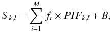 (1)where Sk,l are the detector count rate, PIFk,l are the respective pattern model of source i in the detector pixel with coordinates (k,l), fi,i = 1... M is the flux of source i in the given ScW, and B is the mean background level. This procedure was applied to all the detected sources in the FOV. The stability of the fitting procedure was tested using a large set (>1000) of simulated ScWs with variable source fluxes. The results of the fit were normally distributed around the expected source flux, and therefore we can conclude that our procedure is sufficiently accurate to remove the point sources from the construction of the background maps. The results of the fitting procedure were then used to create a transformed detector image, Ŝk,l, defined as
 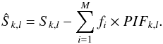 (2)Background maps were then constructed by averaging the transformed detector images of a given data set.
From our time-dependent background maps, we found that the shape of the ISGRI background varies with time, in particular after each solar flare. A long-term change in the background was noticed as well. This result agrees with the findings of Lebrun et al. (2005). To take these variations into account, we generated background maps for each spacecraft revolution and in the image reconstruction step applied them to the extragalactic sky region.
Besides the real physical background of the sky, there is also artificial component, because IBIS/ISGRI is a coded-mask instrument with a periodic mask pattern. Therefore, the deconvolution of ISGRI images creates structures of fake sources that usually appear around bright sources. Apart from the periodicity of the mask, insufficient knowledge of the response function leads to residuals in the deconvolved sky images. The orientation of the spacecraft changes from one observation of the real source to another, so fake sources and structures around the real source contribute to the noise level of the local background. To reduce this contribution, we used a method described in Sect. 2.3.
2.3. Image reconstruction
After producing the background maps as described in the previous subsection, we started the analysis of the data using the standard Offline Scientific Analysis (OSA) package, version 7.0, distributed by ISDC (Courvoisier et al. 2003). For image reconstruction, we used a modified version of the method described in Eckert et al. (2008). It is known that screws and glue strips attaching the IBIS mask to the supporting structure can introduce systematic effects in the presence of very bright sources (Nevalainen et al. 2009). To remove these effects, we identified the mask areas where screws and glue absorb incoming photons, and we disregarded the pixels illuminated by these mask areas for the 11 brightest sources in the hard X-ray band. No more than 1% of the detector area was disregarded for each of the brightest sources. For weaker sources, the level of systematic errors produced by the standard OSA software was found to be consistent with the noise, so the modified method was not required. Finally, we summed all the processed images weighting by variances to create the all-sky mosaic. For this work, we produced mosaics in 3 energy bands (20–40, 40–100, and 100–200 keV). Both our all-sky map images and corresponding exposure maps are available online and we direct the reader to our online web service2. As an example, we provide here the image of the inner part (36° by 12°) of the Galaxy in the 20–40 keV energy band (see Fig. 2).
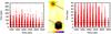 |
Fig. 1 Lightcurves and variability map of HMXB 4U 1700-377 and LMXB GX 349+2. The solid line indicates the mean flux of the sources during the observation time, the dotted line shows the mean flux minus Sint, the dashed line shows the mean flux plus Sint. |
3. Method of variability detection
The variability of INTEGRAL sources can be analyzed in a standard way by studying the inconsistency of the detected signal with that expected from a constant source by performing the χ2 test. Here we consider introducing a variability measurement for the INTEGRAL sources and show how to apply it to the specific case of the coded-mask instrument. For an alternative approach based on the maximum likelihood function for the determination of intrinsic variability of X-ray sources the reader is referred to Almaini et al. (2000) and Beckmann et al. (2007).
The INTEGRAL data are naturally organized by pointings (ScW) with average duration of ~1–3 ks. Therefore, the simplest way to detect the variability of a source on ks and longer timescales is to analyse the evolution of the flux from the source on a ScW-by-ScW basis. We define Fi and  to be the flux and the variance of a given source, respectively, in the ith ScW. The weighted mean flux from the source is then given by
 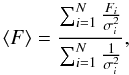 (3)where N is the total number of ScWs. The variance of the source’s flux, which is the mean squared deviation of the flux from its mean value during the observation time, is given by
 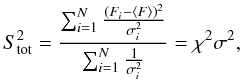 (4)where
  and
and  is the variance of the weighted mean flux.
However, in addition to intrinsic variance of the source, this value includes the uncertainty in the flux measurements during individual ScWs, i.e., the contribution of the noise. If the source variance is caused only by the noise, i.e., Fi = ⟨ F ⟩ ± σi, Eq. (4) is given by  . To eliminate the noise contribution, we can subtract the noise term of the variance from the source variance and derive the intrinsic variance of the source
 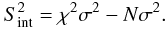 (5)When all measurement errors are equal (σi = σ0,
  ), our case reduces to the method used by Nandra et al. (1997)
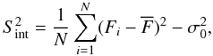 (6)where
  is the unweighted mean flux and
  is called the excess variance. In the absence of measurement errors, our case reduces to the standard definition of the variance
 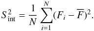 (7)Given that different sources have different fluxes, the variability of sources can be quantified by using the normalized measure of variability, which we call here the fractional variability
  (8)However, in reality, if one were to apply the above method to detect the variable sources in a crowded field (i.e., containing many sources) of a coded-mask instrument such as IBIS, one would infer all the detected sources to be highly variable. This is because in coded-mask instruments, each source casts a shadow of the mask on the detector plane. If there are several sources in the field of view, each of them produces a shadow that is spread over the whole detector plane. Some detector pixels are illuminated by more than one source. If the signal in a detector pixel is variable, one can tell, only with a certain probability, which of the sources illuminating this pixel is responsible for the variable signal. Thus, in a coded-mask instrument, the presence of bright variable sources in the field of view introduces an “artificial” variability for all the other sources illuminating the same pixels. Since the overlap between the PIF of the bright variable source and the sources at different positions on the sky varies with the position on the sky, one is also unable to determine in advance the level of this “artificial” variability in a given region of the deconvolved sky image.
To overcome this difficulty, one has to measure the variability of the flux not only directly in the sky pixels at the position of the source of interest, but also in the background pixels around the source. Obviously, the “artificial” variability introduced by the nearby bright sources is similar in the adjacent background pixels to that in the pixel(s) at the source position. Therefore, one can produce the variability map for the whole sky and compare the values of variability at the position of the source of interest to the mean values of variability in the adjacent background pixels. The variable sources should be visible as local excesses in the variability map of the region of interest. If a source can be localized in the variability image, then the true fractional variability of the source is calculated as 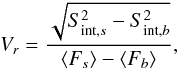 (9)where the subscript b represents the values of the background in the area adjacent to the source and the subscript s the values taken from the source position.
To illustrate the method, we present the lightcurves (Fig. 1) of two objects that are typical bright INTEGRAL sources: the HMXB 4U 1700-377, which is a very bright and very variable source (Vr ≃ 104%), and the LMXB GX 349+2, which is a moderately bright and variable source (Vr ≃ 45%). The solid line indicates the mean flux of the sources, ⟨ F ⟩ . We can see that the mean flux deviation (dotted lines), calculated as the square root of the intrinsic variance, , measures the average flux variation of the sources during the corresponding time. However, we note that in the present case we consider calculations based solely on a lightcurve. If one wishes to obtain a fractional variability value dividing the mean flux deviation by the mean flux, one will obtain the V value, but not Vr, i.e., the contribution of bright variable neighbor sources is not treated properly. It is impossible to extract the variability of the background, Sint,b, and the mean background flux  using the source lightcurve only. A number of lightcurves of the neighboring pixels should also be compiled to estimate Sint,b and . This number should be sufficiently high to obtain good estimates. Therefore, an all-sky approach is justified. In the current example, no sources are much brighter in the vicinity of the ones considered that could strongly affect them, so the difference between V and the catalog Vr value is around 3%, but for the weak sources in the vicinity of bright ones the difference would be higher.
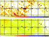 |
Fig. 2 Inner parts (36° by 12°) of the INTEGRAL/ISGRI all-sky maps in Galactic coordinates, Aitoff projection. The significance image (top) in the 20–40 keV energy band, has square root scaling. The bottom image shows the corresponding intrinsic variance map, and also has square root scaling. The circle shows the inner 4° for which the variability background extraction was made from the box region. |
Looking at Eq. (9), one can indeed see that the effect of “artificial” fractional variability is strong for moderate and faint sources in the vicinity of the bright variable sources, while for bright sources the effect is small. The “artificial” variability introduced by the bright sources in their vicinity ( for the surrounding sources) is in range from a fraction of a percent up to a few percent of their own variability (dictated by the PIF accuracy). When we consider the persistent source in the vicinity of the bright variable source,
  is defined by only (i.e., by variability introduced by the bright variable source). For moderate or faint sources, Sint,b may well be comparable to their own flux, and if we apply Eq. (8) directly we will infer substantial fractional variability, which may well be between ten and fifty percent, or even higher. The bright sources are less sensitive to this effect because Sint,b will be only a small fraction of their flux. We checked these conclusions by performing simulations of a moderate persistent source (F = 1 ct/s) in the vicinity of a bright variable source ( ⟨ F ⟩ = 20 ct/s). By applying Eq. (8) directly to measure the fractional variability of a moderate source, we found that V ≃ 25% while Eq. (9) infered that the source was constant, i.e., Vr ≃ 0%.
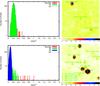 |
Fig. 3 Top: the distributions of the intrinsic variability in pixels of 3.5° × 3.5° area (shown nearby) centered on the IGR J18450-0435. In green is B1 distribution in the range (min,2m − min) here representing the local intrinsic variance background, in red is the sources contribution, f(x) is the Gaussian distribution. Bottom: the 3.5° × 3.5° area (shown nearby) centered on the GC source 1A 1743-288. In green is B1 distribution in the range (min,2m − min), in blue is B2 distribution from the empty region in GC here representing the local intrinsic variance background, in red and f(x) are same as above. |
In the course of simulations, we also checked the behavior of the “artificial” variability in the case a moderate persistent source situated at the ghost position of the bright variable source. We considered two situations: a) when the mosaic image consisted mostly of ScWs in a configuration being determined almost entirely by the spacecraft orientation, which remained constant (i.e., sky region of the Crab), and b) when the mosaic image contained only a chance fraction of ScWs in that specific configuration because of different spacecraft orientations (i.e., sky region of the Cyg X-1). The simulations showed that the flux and therefore the variability measurement of the mosaic deviated from the input source parameters in case a) only, while in case b), there were no significant deviations. As expected in case a), the moderate source was affected. This was caused by the coincidence of the sources shadowgrams. The deconvolution procedure was unable to distinguish the sources correctly on the ScW level, therefore the mosaic results were affected. We detected an incorrect flux and variability for the moderate source. In reality, this particular simulated situation is very rare (see Sect. 5 for discussion of this situation in real case). Even if the constant orientation of some observation is kept, different observation patterns applied during the observation will significantly reduce the undesirable effect considered in situation a).
4. The detection of variable sources
For our study, we used the latest distributed INTEGRAL reference catalog3 (Ebisawa et al. 2003) version 30 and selected the sources with ISGRI_FLAG == 1, i.e., all the sources ever detected by IBIS/ISGRI.
Based on the aforementioned method, we compiled the instrinsic variance maps () of the INTEGRAL sky in three energy bands (20–40, 40–100, and 100–200 keV). This was accomplished by performing pixel operations following Eq. (5) on the constructed all-sky mosaic maps of χ2, σ2 (variance), and N, which is the map showing the number of ScWs used in a given pixel for the all-sky mosaic. As an example, the instrinsic variance image of the inner region of our Galaxy is given in Fig. 2 (see our online service for all-sky maps).
After compiling an intrinsic variance map in each band, we calculated the local (or background) intrinsic variance, , and its scatter, Σ, in the region around each catalog source. This was performed by the following scheme. First, the values of the mean m, the minimum min, and their difference were calculated in a square of 3.5° × 3.5° centered on the source position. We then assumed that the pixel values in the corresponding area are distributed normally and there is the always-positive contribution from the sources in the field. Since the sources occupy a small fraction of the considered sky region, the initial mean value, m, is almost unaffected by their presence because of their small contribution. To reject the source contribution and to obtain the parameters of the normal component, we calculated the mean and the standard deviation in the range (min,2m − min). The newly found mean value is in Eq. (9) and the standard deviation shows its scatter Σ. The detectability of the sources in the intrinsic variance map is then defined by the condition that  . For an illustration (see top of Fig. 3) we present a region around INTEGRAL source IGR J18450-0435 with respective distributions. The green solid area is the distribution in the range (min,2m − min) with the mean value representing for the current source, and in red the always-positive contribution from the sources in the field is given. The distribution in the range (min,2m − min) is well fitted by the Gaussian shown with a dashed line. The top of Fig. 3 justifies well the approximate rejection of the source contribution to the overall pixel value distribution in the field. Applying this rejection procedure allows us to obtain the true scatter in the background rather than the scatter in the overall distribution (including sources), which is obviously higher.
The detection of variable sources in the innermost region of our Galaxy (circle of 4° from the GC, see Fig. 2) was performed differently because it is a crowded field and therefore a large number of sources contribute to the intrinsic variance background of each other. In contrast to the individual source case, the sources in the inner GC region occupy a significant fraction of the region around the source of interest and therefore influence the m value significantly. This results in improper estimation of the background distribution if one applies the rejection procedure based on (min,2m − min) range (B1 distribution at the bottom of Fig. 3). In place of calculating the intrinsic variance background and its scatter for each GC source individually, these values were therefore estimated from an empty field near the GC (box at the bottom image of Fig. 2) and assumed to be equal for all the sources in the GC region. The B2 distribution shown at Fig. 3 (bottom) is accurately determined and well fitted by the Gaussian shown by the dashed line.
5. The catalog of variable sources
The search for variable sources from the reference catalog was performed on the maps generated from ScWs divided into three equal subsequent time periods (maps 1, 2, and 3, approximately 2 years each). This was done to detect transient sources that would be difficult (or even impossible) to detect on the map integrated over the whole time period (map T). The search was performed separately on each map (1, 2, 3) and in each energy band. The results of the search were put into one list from which the sources were selected. Finally, the search was performed on the total map (T) to find sources that were detected only on the map integrated over the whole time period and identify the sources that were active only during specific time periods. The resulting catalog of variable sources detected by INTEGRAL can be found in Table 3.
Figure 4 shows the number of significantly variable sources from our catalog for each source type (HMXB, LMXB, AGN, unidentified, and miscellaneous). The majority of the variable sources (~76%) in all energy bands are Galactic X-ray binaries. We see that in the 100–200 keV band there are four times more LMXBs than HMXBs. The remaining variable sources are AGNs (~10%), unidentified (~7.5%), and other (~6.5%) source types (cataclysmic variables, gamma-ray bursts, and pulsars). The number of significantly variable sources decreases with energy for each population type, which only reflects the sensitivity of the instruments.
The distribution of the variability of sources from Table 3 is presented in Fig. 5. The variability distribution is approximately normal with one evident outlier, the gamma-ray burst IGR J00245+6251 (Vestrand et al. 2005). However, this is mainly caused by the upper limit to the mean flux of this source being too low. The gamma-ray burst IGR J00245+6251 is detected in all three energy bands. Figure 6 shows the fractional variability in the 40–100 keV band versus the variability in the 20–40 keV band. The majority of the sources that are found to be variable in both the 20–40 keV and 40–100 keV energy bands exhibit nearly equal variability in both bands.
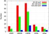 |
Fig. 4 Number of significantly variable sources detected in different energy bands classified by types. |
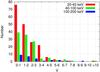 |
Fig. 5 Number of sources versus fractional variability of the sources detected in different energy bands. |
To show the detection threshold for the variability of a source, we compiled a diagram (see Fig. 7) where we plot the fractional variability versus flux for all detected variable sources along with the upper limit to the fractional variability versus flux for all the reference catalog sources detected in our significance map in 20–40 keV energy band. The upper limit was determined by substituting with  in Eq. (9). Although we chose all the sources detected in our significance map, we used the mean flux of the source because, unlike significance, it is an exposure-independent value. According to our definition, the fractional variability is also an exposure-independent value, so we plot it versus the exposure-independent mean flux to clearly see the detection threshold. We can see that starting from a limiting flux (6.2 × 10⁻¹¹ erg/cm2 s or ~10 mCrab) nearly all catalog sources are found to be variable. The majority of the bright sources are binary systems, which explains why nearly all of them are found to be variable.
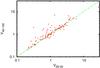 |
Fig. 6 Fractional variability of sources in the 20–40 keV band versus fractional variability in the 40–100 keV band. |
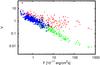 |
Fig. 7 Fractional variability (V) versus flux (F) for all significantly variable sources (red crosses) from Table 3. Energy band is 20–40 keV. For comparison, the green crosses show the fractional variability detection threshold (3-σ) versus flux for all reference catalog sources detected in the significance map. The sources not detected at the variability map are indicated by blue stars and are coincident with their green cross counterparts. Pink squares indicate 3-σ lower limits to the fractional variability of the sources that are not detected in the significance map. |
The transient sources detected at the intrinsic variance map and not detected at the significance map.
Sources with additional error induced by the “ghosts”.
We also found a number of variable sources that have no counterparts in the significance map, which means that we were unable to measure the mean flux of these sources as it is compatible with the background mean flux. Hence, we are not able to give their fractional variability value, which is a normalized value and therefore tends to infinity with infinite errors. For these sources, we provide a 3-σ lower limit to their fractional variability by taking a 3-σ upper limit on their mean flux. Most of the sources are transient, and sometimes (in a specific observation period in a given energy band) the source is not detected in the significance map because the sensitivity of the instrument decreases with energy. Therefore, we can see that the variability map provides a tool to detect transient or faint but variable sources that would be missed in mosaics averaged over long timescales. To illustrate the detectability of the sources in the variability map, we provide a list (see Table 1) of the sources that are smeared out in the significance map because of their high exposures. The values given in the table are not normalized variability values, 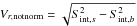 along with their 3-σ errors, Err. To verify that the sources that are absent in the significance maps but detected in the variability maps are not the result of the low detection threshold, we ran the same detection procedures on the mock catalog of 2500 false sources distributed randomly and uniformly over the sky. The test detected 11 of 2500 false sources seen in variability maps and absent from the significance maps, compared to 8 of 576 in the case of the real catalog. This means that our detection criteria are rather strict.
The catalog of variable sources detected by INTEGRAL.
We comment on the inclusion of Crab in our catalog. It is known to be a constant source that is commonly used as a “standard candle” in high-energy astrophysics. There are two reasons why it appears in the catalog. The first is the deterioration of the detector electronics onboard the spacecraft. The loss of detector gain is around 10% over the entire mission. Although this loss is partially compensated by the software, it introduces around 3–5% variability in our method. The remaining variability can be ascribed to systematic errors in the spacecraft alignment (Walter et al. 2003), which for OSA 7.0 are of the order of 7 arcsec (Eckert et al. 2010), hence slightly different positions of the Crab are found in each observation. Since Crab is a very bright source, its Gaussian profile is very steep. When the peak is slightly offset, we measure a sharp decrease in the flux at the catalog position of Crab. The combination of the two effects leads to an artifical variability of Crab in all energy bands. A similar effect occurs in the pixels adjacent to the catalog position of Crab. When the peak of the PSF is found at a slightly displaced position, we find a sharp increase in the flux in this pixel. Our interpretation is confirmed by the image of Crab in the variability map, where the closest pixels to the source are found to be very variable, creating a ring-like structure. Moreover, it has been found that the observed position of Crab does not coincide with the position of the pulsar (Eckert et al. 2010), which thus explains such an effect at the expected source position. To determine the influence of this effect on other sources, we inspected the 11 brightest sources in the 20–40 keV band and looked for a similar situation. In the case of Cyg X-1 and Sco X-1, the same effect, albeit weaker, was also seen. However, the derived value of their variability was not found to be affected by this effect. This effect contributes mainly to the variability of the pixels around the catalog position of these sources. Cyg X-1 and Sco X-1 are intrinsically very variable so the value extracted from the source position is much higher than for surrounding pixels, which is the opposite of the situation found in the Crab. For all the other sources, the influence of the misalignment was found to be negligible.
Finally, we performed a test to find cases in which a source is coincident with the ghost of another source within one ScW (a case described in Sect. 3). We considered all the reference catalog sources and searched for “ghost-source” pairs in individual ScWs from the list used for our all-sky maps. If one of the sources in a given pair was present in our variability catalog, the pair was selected for further analysis. According to our simulations, if two sources are in the ghosts of each other, the fainter one loses up to half of its flux to the flux of the brighter one. If one of the sources is substantially brighter than the other, the relative distortion of the flux of the bright source is minor. Therefore, the flux of the source is significantly distorted if its “ghost companion” is brighter or comparable in brightness to the source itself. In the latter case, the “ghost companion” is also affected. Thus, we assume that if the source in the ghost is more than ten times fainter than its “ghost companion”, its contaminating influence is negligible, whereas its own flux is contaminated significantly. After adopting this condition, we obtained a list of the sources affected by such position coincidences and the exposure times for each of them during which they where affected. For nearly all of the sources from the list, the fraction of exposures with distorted flux is less than 1%, which infers a relative uncertainty in the average flux and fractional variability of the same order. This is much smaller than the error set on variability in our catalog and, as can be seen from the Fig. 7 is smaller than the variability detection threshold even for the brighest sources. Nonetheless, a number of sources have larger than 1% errors induced by the ghosts, which we indicate with a g superscript in the catalog and provide a Table 2 where both errors are given. As can be seen, in all cases the ghost induced error is much smaller than the catalog variability error.
6. The All-Sky online
To make our results available to the community, we decided to take advantage of the SkyView interface (McGlynn et al. 1998) (i.e., a Virtual Observatory service available online5 developed at and hosted by the High Energy Astrophysics Science Archive Research Centre (HEASARC)). SkyView provides a straightforward interface where users can retrieve images of the sky at all wavelengths from radio to gamma-rays (McGlynn et al. 1998). SkyView uses NED and SIMBAD name resolvers to translate names into positions and is connected to the HEASARC catalog services. The user can retrieve images in various coordinate systems, projections, scalings, and sizes as ordinary FITS as well as standard JPEG and GIF file formats. The output image is centered on the queried object or sky position. SkyView is also available as a standalone Java application (McGlynn et al. 1997). The ease-of-use of this system allowed us to incorporate INTEGRAL/ISGRI variability and significance all-sky maps into the SkyView interface. We developed a simple web interface for the SkyView Java application and have made all-sky mosaics available online.
7. Concluding remarks
Our study of variability of the INTEGRAL sky has found that 202 sources exhibit significantly variable hard X-ray emission. To compile the catalog of variable sources, we have developed and implemented a method to detect variable sources, and compiled all-sky variability maps. A search for variable sources from the INTEGRAL reference catalog was carried out in three energy bands: 20–40, 40–100, and 100–200 keV. The variable sources were detected in all studied energy bands, although their number sharply decreases with increasing energy. A number of sources were detected only during specific time periods and not detected on the map integrated over the whole time period. These sources are most likely transient. On the other hand, some sources were found to be variable only on the total variability map. This means that they might be persistent and not extremely variable sources.
We found that around 76% of all variable sources of our catalog are binary systems and nearly 24% of variable sources are either AGNs, unidentified, or other source types. The variability measurements of our catalog sources have rather normal distributions in all energy bands. We found that in the majority of cases the variability of the source in the first band correlates with its variability in the second band. We derived the limits to the fractional variability value to be detected as a function of the source flux (Fig. 7). We also found that variability map can be a tool to detecting transient or faint but variable sources that would be missed in mosaics averaged over long timescales. In a forthcoming paper, we will discuss in more detail the properties of the variable sources detected during this study in order to gain some physical insights into the population of hard X-ray sources.
Finally, we emphasize that the sky maps generated during this study represent 6 years of INTEGRAL operation in orbit. In addition to the variability maps, we have compiled significance maps in three energy bands (20–40, 40–100, and 100–200 keV). All our maps are available as an online service to the community using the SkyView engine.
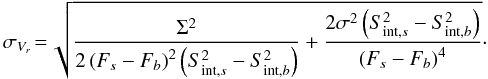
Appendix: Error Calulation on V r
We use the standard error propagation formula to find the error, σVr, of the function
 so:
so:
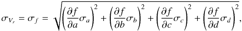 (10)where σa = σb = Σ and σc = σd = σ for a given source. By substituting the appropriate values in Eq. (10) and by taking derivatives we find that:
 (11)
(11)
We used the OSA 7.0 ARFs and RMFs and simulated a source with a Crab-like spectrum. Then using XSPEC we found the conversion between count rate and flux. It should be noted that this method depends on the spectral shape of the source, and that there are several ARFs for different periods of the mission, so the fluxes cannot be fully reliable. However, we find this approach the most suitable for the current catalog paper.
Acknowledgments
Based on observations with INTEGRAL, an ESA project with instruments and science data centre funded by ESA member states (especially the PI countries: Denmark, France, Germany, Italy, Switzerland, Spain), Czech Republic and Poland, and with participation of Russia and the USA. This work was supported by the Swiss National Science Foundation and the Swiss Agency for Development and Cooperation in the framework of the programme SCOPES – Scientific co-operation between Eastern Europe and Switzerland. The computational part of the work was done at VIRGO.UA6 and BITP7 computing resources. We are grateful to the anonymous referee for the critical remarks which helped us improve the paper. I.T. acknowledges the support from the INTAS YSF grant No. 06-1000014-6348.
References
- Almaini, O., Lawrence, A., Shanks, T., et al. 2000, MNRAS, 315, 325 [NASA ADS] [CrossRef] [Google Scholar]
- Arévalo, P., & Uttley, P. 2006, MNRAS, 367, 801 [NASA ADS] [CrossRef] [Google Scholar]
- Barlow, E. J., Knigge, C., Bird, A. J., et al. 2006, MNRAS, 372, 224 [NASA ADS] [CrossRef] [Google Scholar]
- Barnard, R., Kolb, U. C., & Osborne, J. P. 2002, ArXiv Astrophysics e-prints [Google Scholar]
- Bassani, L., Malizia, A., Stephen, J. B., & INTEGRAL AGNs Survey Team 2007, in ESA SP, 622, 165 [Google Scholar]
- Bazzano, A., Stephen, J. B., Fiocchi, M., et al. 2006, ApJ, 649, L9 [NASA ADS] [CrossRef] [Google Scholar]
- Beckmann, V., Gehrels, N., Shrader, C. R., & Soldi, S. 2006, ApJ, 638, 642 [NASA ADS] [CrossRef] [Google Scholar]
- Beckmann, V., Barthelmy, S. D., Courvoisier, T., et al. 2007, A&A, 475, 827 [NASA ADS] [CrossRef] [EDP Sciences] [Google Scholar]
- Beckmann, V., Soldi, S., Ricci, C., et al. 2009, A&A, 505, 417 [NASA ADS] [CrossRef] [EDP Sciences] [Google Scholar]
- Bélanger, G., Goldwurm, A., Goldoni, P., et al. 2004, ApJ, 601, L163 [NASA ADS] [CrossRef] [Google Scholar]
- Bélanger, G., Goldwurm, A., Renaud, M., et al. 2006, ApJ, 636, 275 [Google Scholar]
- Bird, A. J., Malizia, A., Bazzano, A., et al. 2007, ApJS, 170, 175 [NASA ADS] [CrossRef] [Google Scholar]
- Bird, A. J., Bazzano, A., Bassani, L., et al. 2010, ApJS, 186, 1 [NASA ADS] [CrossRef] [Google Scholar]
- Bodaghee, A., Courvoisier, T. J.-L., Rodriguez, J., et al. 2007, A&A, 467, 585 [Google Scholar]
- Bouchet, L., Roques, J. P., Mandrou, P., et al. 2005, ApJ, 635, 1103 [Google Scholar]
- Courvoisier, T. J.-L., Walter, R., Beckmann, V., et al. 2003, A&A, 411, L53 [NASA ADS] [CrossRef] [EDP Sciences] [Google Scholar]
- den Hartog, P. R., Hermsen, W., Kuiper, L., et al. 2006, A&A, 451, 587 [NASA ADS] [CrossRef] [EDP Sciences] [Google Scholar]
- Ducci, L., Sidoli, L., Mereghetti, S., Paizis, A., & Romano, P. 2009, MNRAS, 398, 2152 [NASA ADS] [CrossRef] [Google Scholar]
- Ebisawa, K., Bourban, G., Bodaghee, A., Mowlavi, N., & Courvoisier, T. J.-L. 2003, A&A, 411, L59 [NASA ADS] [CrossRef] [EDP Sciences] [Google Scholar]
- Eckert, D., Produit, N., Paltani, S., Neronov, A., & Courvoisier, T. J.-L. 2008, A&A, 479, 27 [NASA ADS] [CrossRef] [EDP Sciences] [Google Scholar]
- Eckert, D., Savchenko, V., Produit, N., & Ferrigno, C. 2010, A&A, 509, A33 [NASA ADS] [CrossRef] [EDP Sciences] [Google Scholar]
- Götz, D., Mereghetti, S., Merlini, D., Sidoli, L., & Belloni, T. 2006, A&A, 448, 873 [NASA ADS] [CrossRef] [EDP Sciences] [Google Scholar]
- Gros, A., Goldwurm, A., Cadolle-Bel, M., et al. 2003, A&A, 411, L179 [NASA ADS] [CrossRef] [EDP Sciences] [Google Scholar]
- Ishibashi, W., & Courvoisier, T. 2009, A&A, 504, 61 [NASA ADS] [CrossRef] [EDP Sciences] [Google Scholar]
- Krivonos, R., Revnivtsev, M., Churazov, E., et al. 2007, A&A, 463, 957 [NASA ADS] [CrossRef] [EDP Sciences] [Google Scholar]
- Lebrun, F., Leray, J. P., Lavocat, P., et al. 2003, A&A, 411, L141 [NASA ADS] [CrossRef] [EDP Sciences] [Google Scholar]
- Lebrun, F., Roques, J., Sauvageon, A., et al. 2005, Nucl. Instrum. Methods Phys. Res. A, 541, 323 [Google Scholar]
- Liang, E. W., & Liu, H. T. 2003, MNRAS, 340, 632 [NASA ADS] [CrossRef] [Google Scholar]
- Lund, N., Budtz-Jørgensen, C., Westergaard, N. J., et al. 2003, A&A, 411, L231 [NASA ADS] [CrossRef] [EDP Sciences] [Google Scholar]
- Mas-Hesse, J. M., Giménez, A., Culhane, J. L., et al. 2003, A&A, 411, L261 [NASA ADS] [CrossRef] [EDP Sciences] [Google Scholar]
- McGlynn, T., Scollick, K., & White, N. 1998, in New Horizons from Multi-Wavelength Sky Surveys, ed. B. J. McLean, D. A. Golombek, J. J. E. Hayes, & H. E. Payne, IAU Symp., 179, 465 [Google Scholar]
- McGlynn, T. A., Scollick, K. A., & White, N. E. 1997, in Astronomical Society of the Pacific Conference Series, Astronomical Data Analysis Software and Systems VI, ed. G. Hunt, & H. Payne, 125, 337 [Google Scholar]
- Molkov, S. V., Cherepashchuk, A. M., Lutovinov, A. A., et al. 2004, Astron. Lett., 30, 534 [NASA ADS] [CrossRef] [Google Scholar]
- Nandra, K., George, I. M., Mushotzky, R. F., Turner, T. J., & Yaqoob, T. 1997, ApJ, 476, 70 [NASA ADS] [CrossRef] [Google Scholar]
- Nevalainen, J., Eckert, D., Kaastra, J., Bonamente, M., & Kettula, K. 2009, A&A, 508, 1161 [NASA ADS] [CrossRef] [EDP Sciences] [Google Scholar]
- Revnivtsev, M. G., Sunyaev, R. A., Varshalovich, D. A., et al. 2004, Astron. Lett., 30, 382 [NASA ADS] [CrossRef] [Google Scholar]
- Romano, P., Sidoli, L., Cusumano, G., et al. 2009, MNRAS, 1437 [Google Scholar]
- Sazonov, S., Revnivtsev, M., Krivonos, R., Churazov, E., & Sunyaev, R. 2007, A&A, 462, 57 [NASA ADS] [CrossRef] [EDP Sciences] [Google Scholar]
- Ubertini, P., Lebrun, F., Di Cocco, G., et al. 2003, A&A, 411, L131 [NASA ADS] [CrossRef] [EDP Sciences] [Google Scholar]
- Uttley, P. 2004, MNRAS, 347, L61 [NASA ADS] [CrossRef] [Google Scholar]
- Vedrenne, G., Roques, J.-P., Schönfelder, V., et al. 2003, A&A, 411, L63 [NASA ADS] [CrossRef] [EDP Sciences] [Google Scholar]
- Vestrand, W. T., Wozniak, P. R., Wren, J. A., et al. 2005, Nature, 435, 178 [NASA ADS] [CrossRef] [PubMed] [Google Scholar]
- Walter, R., Favre, P., Dubath, P., et al. 2003, A&A, 411, L25 [NASA ADS] [CrossRef] [EDP Sciences] [Google Scholar]
- Winkler, C., Courvoisier, T. J.-L., Di Cocco, G., et al. 2003, A&A, 411, L1 [NASA ADS] [CrossRef] [EDP Sciences] [Google Scholar]
All Tables
The transient sources detected at the intrinsic variance map and not detected at the significance map.
All Figures
|
Fig. 1 Lightcurves and variability map of HMXB 4U 1700-377 and LMXB GX 349+2. The solid line indicates the mean flux of the sources during the observation time, the dotted line shows the mean flux minus Sint, the dashed line shows the mean flux plus Sint. |
| In the text | |
|
Fig. 2 Inner parts (36° by 12°) of the INTEGRAL/ISGRI all-sky maps in Galactic coordinates, Aitoff projection. The significance image (top) in the 20–40 keV energy band, has square root scaling. The bottom image shows the corresponding intrinsic variance map, and also has square root scaling. The circle shows the inner 4° for which the variability background extraction was made from the box region. |
| In the text | |
|
Fig. 3 Top: the distributions of the intrinsic variability in pixels of 3.5° × 3.5° area (shown nearby) centered on the IGR J18450-0435. In green is B1 distribution in the range (min,2m − min) here representing the local intrinsic variance background, in red is the sources contribution, f(x) is the Gaussian distribution. Bottom: the 3.5° × 3.5° area (shown nearby) centered on the GC source 1A 1743-288. In green is B1 distribution in the range (min,2m − min), in blue is B2 distribution from the empty region in GC here representing the local intrinsic variance background, in red and f(x) are same as above. |
| In the text | |
|
Fig. 4 Number of significantly variable sources detected in different energy bands classified by types. |
| In the text | |
|
Fig. 5 Number of sources versus fractional variability of the sources detected in different energy bands. |
| In the text | |
|
Fig. 6 Fractional variability of sources in the 20–40 keV band versus fractional variability in the 40–100 keV band. |
| In the text | |
|
Fig. 7 Fractional variability (V) versus flux (F) for all significantly variable sources (red crosses) from Table 3. Energy band is 20–40 keV. For comparison, the green crosses show the fractional variability detection threshold (3-σ) versus flux for all reference catalog sources detected in the significance map. The sources not detected at the variability map are indicated by blue stars and are coincident with their green cross counterparts. Pink squares indicate 3-σ lower limits to the fractional variability of the sources that are not detected in the significance map. |
| In the text | |
Current usage metrics show cumulative count of Article Views (full-text article views including HTML views, PDF and ePub downloads, according to the available data) and Abstracts Views on Vision4Press platform.
Data correspond to usage on the plateform after 2015. The current usage metrics is available 48-96 hours after online publication and is updated daily on week days.
Initial download of the metrics may take a while.