| Issue |
A&A
Volume 708, April 2026
|
|
|---|---|---|
| Article Number | L16 | |
| Number of page(s) | 8 | |
| Section | Letters to the Editor | |
| DOI | https://doi.org/10.1051/0004-6361/202659316 | |
| Published online | 17 April 2026 | |
Letter to the Editor
Perihelion observations of interstellar comet 3I/ATLAS with the IRAM 30-m telescope★
1
LIRA, Observatoire de Paris, PSL Research University, CNRS, Sorbonne Université, Université de Paris, 5 place Jules Janssen, F-92195, Meudon, France
2
IRAM, Avd. Divina Pastora, 7, 18012, Granada, Spain
3
IRAM, 300, rue de la Piscine, F-38406, Saint Martin d’Hères, France
4
NASA Goddard Space Flight Center, 8800 Greenbelt Road, Greenbelt, MD, 20771, USA
5
Department of Physics, Catholic University of America, 620 Michigan Ave. NE, Washington, DC, 20064, USA
6
Department of Physics, American University, 4400 Massachusetts Ave NW, Washington, DC, 20016, USA
★★ Corresponding author: This email address is being protected from spambots. You need JavaScript enabled to view it.
Received:
4
February
2026
Accepted:
23
March
2026
Abstract
Comet 3I/ATLAS is the third interstellar comet identified as passing through the Solar System. Its high outgassing activity and favourable perihelion passage on October 29, 2025 UT provided an excellent opportunity to investigate the composition of its coma gases through millimeter spectroscopy. We present observations undertaken with the IRAM 30-m telescope on November 1–3, 2025 at an heliocentric distance of 1.36–1.37 au. Lines of HCN, CH3OH, CO, and H2CO are well detected, and ∼4σ detections are obtained for CS and CH3CN. The search for H2S was unsuccessful. Abundances of CO, H2CO, CH3OH, and CH3CN relative to HCN are in the upper ranges of values measured in Solar System comets. The sulfur-to-carbon abundance ratio in 3I/ATLAS’s coma is at most the minimum value observed in comets. The unusually low expansion velocity of coma gases suggests a near-nucleus gas flow driven by heavy molecules such as CO2, and/or a large fraction of the gaseous production coming from subliming icy grains.
Key words: comets: general / comets: individual: 3I/ATLAS
Based on observations carried out with the IRAM 30-m telescope. IRAM is supported by INSU/CNRS (France), MPG (Germany) and IGN (Spain).
© The Authors 2026
 Open Access article, published by EDP Sciences, under the terms of the Creative Commons Attribution License (https://creativecommons.org/licenses/by/4.0), which permits unrestricted use, distribution, and reproduction in any medium, provided the original work is properly cited.
This article is published in open access under the Subscribe to Open model. This email address is being protected from spambots. You need JavaScript enabled to view it. to support open access publication.
1. Introduction
Comets are fingerprints of the formation of planetary systems. Water and the numerous complex molecules composing the ices of their nucleus were likely synthesized in the molecular cloud precursor of the Solar System (Altwegg et al. 2019; Ceccarelli et al. 2023; Biver et al. 2024b). The passing of a bright cometary-like interstellar object through the Solar System was long awaited to investigate the physical and chemical properties of icy planetesimals in other planetary systems. The first interstellar object, 1I/’Oumuamua, was discovered in October 2017 a few days after its closest approach to Earth. There was no detection of coma gases and dust particles (’Oumuamua ISSI Team 2019, and references therein), but astrometric measurements suggested the presence of non-gravitational forces related to cometary activity (Micheli et al. 2018). The second interstellar object 2I/Borisov, discovered in 2019, showed cometary activity and was extensively observed. Several simple volatile species commonly observed in Solar System comets (OH, C2, CN, HCN, NH, NH2, CO, Ni, Fe) were detected (e.g., Opitom et al. 2019, 2021; Cordiner et al. 2020; Deam et al. 2025). Spectroscopic properties and mixing ratios were found to be remarkably similar to Solar System comets. Comet 2I/Borisov was found to be carbon-chain depleted, similar to the class of carbon-chain depleted comets of Solar System origin (Opitom et al. 2019; Kareta et al. 2020; Lin et al. 2020). However, a high enrichment in CO relative to H2O was revealed, suggesting specific formation conditions in its natal protoplanetary disk (Bodewits et al. 2020; Cordiner et al. 2020).
In this letter, we report on spectroscopic observations with the 30-m telescope of the Institut de radioastronomie millimétrique (IRAM) of the third identified interstellar object, 3I/ATLAS (also named 3I/2025 N1 (ATLAS)), which were performed near its perihelion on October 29.48, 2025 UT, at rh = 1.356 au from Sun. This interstellar object was discovered with the robotic telescope ATLAS in Chile on July 1, 2025, as it was at 5 au from the Sun, and was confirmed to be a comet the day after (CBET 5578, Seligman et al. 2025). Subsequent studies have revealed a fast increase of its gaseous activity as it approached the Sun, making the detection of molecular species at millimeter wavelengths possible. Detections of HCN and CH3OH were reported from observations with the James Clerk Maxwell Telescope at rh = 2.1 au (Coulson et al. 2026) and rh = 1.39 au (Kuan et al. 2025), respectively. The HCN and CH3OH molecular lines were mapped with the ALMA Compact Array (ACA) in a time range spanning 2.6–1.7 au pre-perihelion, from which it was inferred that the CH3OH/HCN ratio in 3I/ATLAS is among the largest values measured in any comet (Roth et al. 2026). In this letter, we present the detection of HCN, CH3OH, CO, H2CO, CH3CN and CS at rh = 1.36–1.37 au (November 1–3, 2025). Sensitive upper limits for several molecules, including HNC and H2S, were also obtained. We compare abundance ratios in 3I/ATLAS to values measured in Solar System comets and discuss the unique dynamic properties of the coma gases.
2. Observations
The observations were conducted with the IRAM 30-m telescope (Sierra Nevada, Spain) from November 1 to 3, 2025, as Director Discretionary Time (DDT D05-25). Comet 3I/ATLAS was at that time at rh ∼ 1.36 au from the Sun and Δ ∼ 2.27 au from Earth (Table A.1). The EMIR 150 GHz and 230 GHz dual-side band receivers were used, with two distinct tunings for the latter. Each of the three setups covered 8 GHz in each side band. The setup with the 150 GHz receiver targeted the H2S 110– 101 (168.8 GHz) and CS J(3–2) (147 GHz) lines. One 230 GHz setup was optimized to look for HCN J(3–2) at 265.9 GHz in the upper side band (USB) and lines of the CH3OH 252 GHz multiplet in the lower sideband (LSB). The other 230 GHz setup was designed to target CO J(2–1) (230.5 GHz) and H2CO 312–211 (225.7 GHz) in LSB and some of the strongest methanol lines near 242 GHz and the CS J(5–4) (244.9 GHz) line in USB. As backends, we used the fast Fourier transform spectrometer (resolution of 200 kHz) and the VESPA autocorrelator (resolution of 40 kHz) in parallel.
The three setups were executed each day (Table A.1). The first day offered low opacity conditions, below 2 mm precipitable water vapour (pwv), but the weather was unstable and windy (resulting in an 1.1 h-long interruption). The next day started with a high opacity (11 mm pwv), which decreased with time, but a good focus and pointing was again difficult to obtain, especially at the beginning of the observations during sunrise, when the source was at low elevation. On the third day the opacity was relatively good (3–4 mm pwv), and the pointing and focus were generally more reliable. The pointing errors, including those related to the used ephemeris, were estimated afterwards and found to be ∼3″ for most observations (Table B.1). The telescope beam size is 10.8″ at 230.5 GHz.
3. Results
Figures 1 and 2 show sample spectra of comet 3I/ATLAS. A list of detected lines is given in Table B.1 together with their line areas in main-beam brightness temperature scale. The HCN, CO, and H2CO lines are well detected. CH3OH is detected through multiple lines (> 30), including with the 150 GHz receiver. Two CS lines are marginally detected, at 3.3σ for J(5–4), and 2.3σ for J(2–1). The CH3CN J(8–7) (147 GHz) and J(9–8) (166 GHz) lines are detected at 3σ and 2.5σ, respectively. Combining the different lines, CS and CH3CN are detected at 4σ. A marginal detection, slightly below 3σ, was also obtained for HNC. The J(3–2) HCO+ line (267.6 GHz) is also marginally seen. However, H2S was not detected. The large bandwidth of EMIR receivers allowed us to search for many species, including by using line stacking, so Tables B.1 and 1 include upper limits for many species observed in cometary atmospheres, including deuterated species.
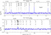 |
Fig. 1. Methanol lines near 242 GHz and 252 GHz observed in comet 3I/ATLAS on November 1–3, 2025. |
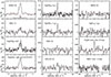 |
Fig. 2. Sample of spectra obtained in comet 3I/ATLAS on November 1–3, 2025. Line characteristics are given in Table B.1. The plot with the HCN J(3–2) spectrum shows the position and relative intensities of the hyperfine components. |
Production rates and abundances in comet 3I/ATLAS on November 1–3, 2025.
In order to derive production rates, we followed the approach used in previous papers (e.g., Biver et al. 2021, 2024a, and references therein). The expansion velocity was estimated from the line profiles. The HCN, CO and CH3OH lines observed at high spectral resolution have similar slightly blueshifted (Δv ≈ −0.05 km s−1 on average) line shapes (Fig. 2, Table B.1). Gaussian fits to the lines yielded on average half widths of VHM = 0.54 ± 0.04 and 0.34 ± 0.02 km s−1 in the blue and red wings of the profiles, respectively (Table G.1). A model considering asymmetric outgassing with expansion velocities of 0.42 and 0.32 km s−1 in the sunward and antisunward hemispheres provided a good fit to the line profiles (Fig. C.1). Isotropic outgassing at an expansion velocity of 0.37 km s−1 yields the same production rates, so this approximation was used.
In the excitation model, which considers both collisional excitation by water and electrons as well as radiative processes, we assumed a constant kinetic temperature and an electron-density scaling factor xne = 0.5 (Biver 1997). With a kinetic temperature of 60 K, the rotational temperatures derived from the modeled CH3OH line intensities are consistent with the values derived from the observations of the CH3OH multiplets (Fig. 1): Trot(165 Hz) = 44.5 ± 3.5 K, Trot(252 GHz) = 48 ± 5 K (see rotation diagram in Fig. D.1), and Trot(242 GHz) = 29 ± 1.5 K. In Solar System comets, the spatial distribution of H2CO cannot be explained by a direct release from the nucleus and suggests production from the dust grains. For this species, we adopted a Haser daughter distribution to describe the radial evolution of the H2CO number density. The parent scale length was set to Lp = 2000 km (i.e., 0.5 times the H2CO photodissociative scalelength) based on measurements in Solar System comets (Roth et al. 2021; Biver et al. 2024a). The derived H2CO production rate is not significantly dependent on the assumed Lp since the beam size is large (∼17 000 km diameter at the frequency of the H2CO line)1. For SO and CS, we assumed Lp = 3000 km and 1700 km, respectively (Biver et al. 2024a). For other molecules (except HCO+, which we do not consider in the analysis), we assumed direct release from the nucleus. Derived production rates (or their upper limits) are listed in Table 1.
The determination of mixing ratios with respect to water relies on contemporaneous observations of H2O or of its photodissociation products (OH, H). Bockelée-Morvan et al. (2026) report QH2O = (6.58 ± 0.13)×1028 molec. s−1 on November 2 from infrared H2O data with a 3 × 3′ field of view obtained with the Moons And Jupiter Imaging Spectrometer (MAJIS) on board the Jupiter Icy Moons Explorer (JUICE). On the other hand, Combi et al. (2026), from Lyman-α data obtained with SOHO/SWAN, report a large water production rate of QH2O = 3.2 × 1029 molec. s−1 at 1.4 au post-perihelion (November 6)2. The large field of view of SOHO/SWAN was possibly sensitive to large-scale water production from subliming icy grains. Extended water production from icy grains (i.e., hyperactivity) at perihelion is suggested from the icy area fraction (see Lis et al. 2019) of ∼900% at 1.4 au that we derived from the QH2O measured by SOHO/SWAN and setting a nucleus radius of 1.3 km as inferred from HST observations (Hui et al. 2026). To interpret the IRAM data (∼11″ field of view), we used the QH2O value of 6.6 × 1028 molec. s−1 deduced from the MAJIS data. Observations of OH 18-cm lines at the Nançay radio telescope (3.5′ × 19′ beam) yielded QOH = (7.0 ± 0.6)×1028 molec. s−1 for October 13–19 (rh = 1.43 au) (Crovisier et al. 2025)3 and QOH = (6.1 ± 1.4)×1028 molec. s−1 for November 18–22 (rh = 1.57 au).
Derived production rates and mixing ratios can be compared to pre-perihelion measurements from when the comet was farther from the Sun. The CO/H2O mixing ratio at rh = 1.36 au (∼10%) is much lower than the value at 3.32 au (∼165%) derived from JWST observations (Cordiner et al. 2025b). This is not surprising, as water sublimation is not efficient at rh ≥ 3 au. The CH3OH production rate at rh = 1.36 au is a factor of two lower than the trend with rh established from ACA observations in the range 2.6–1.7 au (Roth et al. 2026), suggesting that the activity of 3I/ATLAS leveled off when approaching perihelion. The CH3OH/H2O ratio (5.1 ± 0.1%) is, within 1.5σ, consistent with the pre-perihelion (rh = 1.43 au) value of 8 ± 2% derived by Roth et al. (2026).
4. Discussion
The molecular species detected in this millimeter spectral survey of 3I/ATLAS are those which are commonly observed in Solar System comets (e.g., Biver et al. 2024a,b), indicating that the parent protoplanetary disk (and natal molecular cloud) of this icy object share the same chemical properties, at least at a first approximation. However, the derived abundances in 3I/ATLAS’s coma are somewhat different from those of Solar System comets (Table 1). The first striking difference is the low (∼0.06%) HCN/H2O mixing ratio. For comparison, the HCN/H2O ratio measured in the radio is ∼0.1% for most Solar System comets (Biver et al. 2024b). Also, striking is the low CS abundance, which is in the low end of the range of values in Solar System comets. On the other hand, CO/H2O and CH3OH/H2O are enhanced with respect to the mean abundances in Solar System comets, while H2CO/H2O and CH3CN/H2O are typical (Fig. E.1). From histograms of the abundance ratios with respect to HCN (Fig. 3), 3I/ATLAS displays high CO/HCN, H2CO/HCN, CH3OH/HCN, and CH3CN/HCN abundance ratios and a rather low CS/HCN ratio. As concluded by Roth et al. (2026), 3I/ATLAS’s coma is especially highly enriched in its CH3OH/HCN abundance, being only surpassed by the peculiar CO-rich and N2-rich comet C/2016 R2 (PanSTARRS). It would be tempting to conclude to a high elemental C/N ratio in 3I/ATLAS nuclear ices, but HCN is not the dominant carrier of nitrogen in cometary ices (Biver et al. 2024b). Figure F.1 shows a histogram of the ratio of the total abundance of sulfur-bearing species to the total abundance of carbon-bearing molecules in comets, considering only the CO, CH3OH, H2CO, CS and H2S molecules observed in 3I/ATLAS. The value for 3I/ATLAS is at most the minimum value observed in comets, illustrating the peculiar chemistry of this interstellar object.
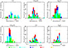 |
Fig. 3. Histograms of the abundances relative to HCN measured from observations at radio wavelengths. Dynamically new (DN) and long-period (LP) comets from the Oort cloud (OCC), Halley-family comets (HFC) and Jupiter-family comets (JFC) are indicated in green, cyan, blue, and red colors, respectively. The orange color is for 3I/ATLAS. See Biver et al. (2024b) and references therein. |
From the observation of the HDO line at 241.56 GHz (Table B.1), we derived an upper limit for the D/H in H2O of < 0.91% (at 3σ). This value is a factor of 10 or more higher than the value measured in comets (e.g., Müller et al. 2022; Biver et al. 2024b; Cordiner et al. 2025a). For CH3OH, we obtained an upper limit on the D/H value of 5.3% by stacking 17 CH3OD lines between 226 and 272 GHz. This is a factor of 4 larger than the value measured in comet 67P (Drozdovskaya et al. 2021), thereby excluding extreme deuteration levels for this molecule in 3I/ATLAS.
Perhaps, the most surprising property of 3I/ATLAS’s coma is the very low expansion velocity, which is a factor of two below the value of ∼0.7–0.8 km s−1 measured in comets of similar activity levels and at comparable heliocentric distances. This low velocity might be the signature of a gas flow dominated by heavy molecules such as CO2 (Fig. G.1). This molecule was found to be overabundant in 3I/ATLAS at 3.3 au (Cordiner et al. 2025b). Comet 3I/ATLAS would then share similarities with the hyperactive comet 103P/Hartley 2, whose nucleus released large amounts of CO2 at its perihelion, dragging water ice grains and chunks that subsequently sublimated in the coma (A’Hearn et al. 2011). The amounts of water and CO2 molecules released from the nucleus of 103P/Hartley 2 are comparable (Fougere et al. 2013), which might explain why the gas expansion velocity in this comet (0.6 km s−1, Hartogh et al. 2011) was not abnormally low (Appendix G, Fig. G.1). Alternatively, the low velocity measured in 3I/ATLAS could be directly related to a large amount of coma gases released from icy grains. This is predicted by gas flow kinetic models including release both from the nucleus and from icy grains using a direct simulation Monte Carlo approach, and the effect is all the more significant since the amount of icy grains is high (Fougere et al. 2012).
In conclusion, the observations of comet 3I/ATLAS with the IRAM 30-m telescope allowed us to identify six molecules in its coma with relative abundances that are at the extreme ends of the range of values measured in Solar System comets. Advanced modelling is needed to understand the unique dynamic properties of the atmosphere of this comet.
References
- A’Hearn, M. F., Belton, M. J. S., Delamere, W. A., et al. 2011, Science, 332, 1396 [CrossRef] [Google Scholar]
- Altwegg, K., Balsiger, H., & Fuselier, S. A. 2019, ARA&A, 57, 113 [NASA ADS] [CrossRef] [Google Scholar]
- Biver, N. 1997, Ph.D. Thesis, Université Paris VII [Google Scholar]
- Biver, N., Bockelée-Morvan, D., Boissier, J., et al. 2021, A&A, 648, A49 [EDP Sciences] [Google Scholar]
- Biver, N., Bockelée-Morvan, D., Handzlik, B., et al. 2024a, A&A, 690, A271 [NASA ADS] [CrossRef] [EDP Sciences] [Google Scholar]
- Biver, N., Dello Russo, N., Opitom, C., et al. 2024b, in Comets III, eds. K. J. Meech, M. R. Combi, D. Bockelée-Morvan, S. N. Raymond & M. E. Zolensky (University of Arizona Press), 459 [Google Scholar]
- Bockelée-Morvan, D., Langevin, Y., Poulet, F., et al. 2026, ATel, 17726 [Google Scholar]
- Bodewits, D., Noonan, J. W., Feldman, P. D., et al. 2020, Nat. Astron., 4, 867 [Google Scholar]
- Ceccarelli, C., Codella, C., Balucani, N., et al. 2023, Protostars and Planets VII, 534, 379 [NASA ADS] [Google Scholar]
- Combi, M. R., Mäkinen, T., Bertaux, J. L., et al. 2026, ApJ, 998, L17 [Google Scholar]
- Cordiner, M. A., Milam, S. N., Biver, N., et al. 2020, Nat. Astron., 4, 861 [Google Scholar]
- Cordiner, M. A., Gibb, E. L., Kisiel, Z., et al. 2025a, Nat. Astron., 9, 1476 [Google Scholar]
- Cordiner, M. A., Roth, N. X., Kelley, M. S. P., et al. 2025b, ApJ, 991, L43 [Google Scholar]
- Coulson, I. M., Kuan, Y. J., Charnley, S. B., et al. 2026, MNRAS, 546, stag063 [Google Scholar]
- Crovisier, J., Biver, N., & Bockelée-Morvan, D. 2025, CBET, 5625 [Google Scholar]
- Deam, S. E., Bannister, M. T., Opitom, C., et al. 2025, arXiv e-prints [arXiv:2507.05051] [Google Scholar]
- Drozdovskaya, M. N., Schroeder, I. I. R. H. G., Rubin, M., et al. 2021, MNRAS, 500, 4901 [Google Scholar]
- Fougere, N., Combi, M. R., Tenishev, V., et al. 2012, Icarus, 221, 174 [NASA ADS] [CrossRef] [Google Scholar]
- Fougere, N., Combi, M. R., Rubin, M., et al. 2013, Icarus, 225, 688 [NASA ADS] [CrossRef] [Google Scholar]
- Hartogh, P., Lis, D. C., Bockelée-Morvan, D., et al. 2011, Nature, 478, 218 [Google Scholar]
- Hui, M.-T., Jewitt, D., Mutchler, M. J., et al. 2026, ApJ, 999, L37 [Google Scholar]
- Kareta, T., Andrews, J., Noonan, J. W., et al. 2020, ApJ, 889, L38 [Google Scholar]
- Kuan, Y. J., Chuang, Y. L., Coulson, I. M., et al. 2025, CBET, 5628 [Google Scholar]
- Lin, H. W., Lee, C.-H., Gerdes, D. W., et al. 2020, ApJ, 889, L30 [Google Scholar]
- Lis, D. C., Bockelée-Morvan, D., Güsten, R., et al. 2019, A&A, 625, L5 [NASA ADS] [CrossRef] [EDP Sciences] [Google Scholar]
- Micheli, M., Farnocchia, D., Meech, K. J., et al. 2018, Nature, 559, 223 [Google Scholar]
- Müller, D. R., Altwegg, K., Berthelier, J. J., et al. 2022, A&A, 662, A69 [NASA ADS] [CrossRef] [EDP Sciences] [Google Scholar]
- Opitom, C., Fitzsimmons, A., Jehin, E., et al. 2019, A&A, 631, L8 [NASA ADS] [CrossRef] [EDP Sciences] [Google Scholar]
- Opitom, C., Jehin, E., Hutsemékers, D., et al. 2021, A&A, 650, L19 [EDP Sciences] [Google Scholar]
- ’Oumuamua ISSI Team, Bannister, M. T., Bhandare, A., et al. 2019, Nat. Astron., 3, 594 [NASA ADS] [CrossRef] [Google Scholar]
- Roth, N. X., Milam, S. N., Cordiner, M. A., et al. 2021, ApJ, 921, 14 [NASA ADS] [CrossRef] [Google Scholar]
- Roth, N. X., Cordiner, M. A., Bockelée-Morvan, D., et al. 2026, ApJ, 999, L32 [Google Scholar]
- Seligman, D. Z., Micheli, M., Farnocchia, D., et al. 2025, ApJ, 989, L36 [Google Scholar]
- Tan, H., Yan, X., & Li, J.-Y. 2026, ApJ, 998, L22 [Google Scholar]
- Zakharov, V. V., Rodionov, A. V., Fulle, M., et al. 2021, Icarus, 354, 114091 [NASA ADS] [CrossRef] [Google Scholar]
- Zakharov, V. V., Rotundi, A., Bockelée-Morvan, D., et al. 2023, Icarus, 395, 115453 [Google Scholar]
The ACA observations suggest that H2CO is more extended in 3I/ATLAS (M. Cordiner, personal communication). A production rate 9% and 18% higher than given in Table 1 is obtained for Lp = 6000 and 8000 km, respectively.
Tan et al. (2026) report QPH2O values five to six times smaller using the same SOHO/SWAN data set but also conclude that 3I/ATLAS is an hyperactive comet. Still unpublished MAVEN data are consistent with results from Combi et al. (2026) (J. Deighan, personal communication).
Updated value from a reevaluation of the maser inversion.
Appendix A: Log of the observations
Log of observations.
Appendix B: Detected lines and their characteristics
Line intensities from IRAM observations
Appendix C: Synthetic line profiles
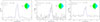 |
Fig. C.1. Synthetic line profiles (blue) superimposed on observed line profiles (black) of HCN (left panel) and CH3OH (middle and right panels). The inserts in the upper right of the plots show the assumed geometry of the outgassing with respect to the Sun direction, with the production rates given in units of 1025 molec. s−1 for HCN, and in units of 1026 molec. s−1 for CH3OH. The assumed expansion velocities (km s−1) in the sunward and antisunward hemispheres are also indicated. Thermal broadening assuming a kinetic temperature of 60 K (see main text) is considered. |
Appendix D: CH3OH rotation diagram
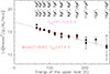 |
Fig. D.1. Rotation diagram of CH3OH, using J3 − J3A+ and A− lines near 252 GHz. Red circles show the output of the excitation model assuming a kinetic temperature of 60 K. It reproduces nicely the measured rotational temperature of 47.7±5.2 K. The labels of the upper levels of the transitions are given at the top of the plot. |
Appendix E: Histograms of abundances relative to water
Appendix F: Histogram of the sulfur-carbon ratio
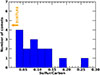 |
Fig. F.1. Histograms of the sulfur to carbon abundance ratio measured from observations at radio wavelengths. Considered sulfur and carbon-bearing molecules are CO, CH3OH, H2CO, H2S and CS. Only comets for which these five species are detected are considered. Note however that H2CO has a minor abundance, compared to CH3OH and CO, and CS is much less abundant than H2S in most comets. The upper limit for 3I/ATLAS is shown by an orange arrow. See Biver et al. (2024b) and references therein. |
Appendix G: Expansion velocity
Figure G.1 compares the expansion velocity measured in 3I/ATLAS from molecular line profiles to the gas velocity expected in three limiting cases.
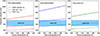 |
Fig. G.1. Initial velocity V0, maximal velocity Vmax, and terminal velocity for free-molecular expansion Vfree as a function of source temperature (TN). From left to right, CO2-dominated, H2O-dominated, and H2O-CO2 gas mixture. The range for 3I/ATLAS (in blue) delineates the expansion velocities measured in the blue and red wings of the line profiles (i.e. VHM values, see main text). |
Line widths
We define the gas initial velocity V0 as the sonic velocity:
 (G.1)
(G.1)
where γ is the specific heat ratio (equal to 1.33 for H2O, 1.28 for CO2), T0 is the gas temperature at sonic line (equal to ∼ 0.82 times the temperature of the source releasing gases, referred to as TN), and mg is the molecular mass of expanding gases.
The maximal terminal gas velocity, which is reached in case of complete transfer of initial thermal energy into kinetic energy of the flow, is (e.g., Zakharov et al. 2021)
 (G.2)
(G.2)
This terminal velocity is almost reached only for active comets, with large regions of fluid flow. This is shown by Zakharov et al. (2023) who studied flow conditions from fluid to free molecular using a kinetic approach (direct simulation Monte Carlo method, so-called DSMC).
The maximum velocity reached in free-molecular expansion (i.e., in case of very weak gas production) is
 (G.3)
(G.3)
In Figure G.1, we consider comas dominated by H2O, by CO2, and composed of both gases in equal quantities (mg = 31 g/mole, γ = 1.3). Calculations are made for source temperatures from 200 K (temperature of exposed ice at typically rh = 1 au) to 300 K (appropriate if one considers gas diffusion through a layer of warm non-ice material). For an H2O-dominated coma, Vmax is close to the typical expansion velocity of 0.7–0.8 km s−1 measured in moderatly active comets (QH2O = 1028–1029 molec. s−1). This outgassing regime is excluded for 3I/ATLAS. The measured velocities are consistent with an H2O-dominated outgassing only in the case of very weak water production (with free molecular expansion)(Fig. G.1, central panel). A CO2-rich coma is favored as in this case the expected gas expansion velocity is significantly lower (Fig. G.1, left and right panels).
All Tables
All Figures
|
Fig. 1. Methanol lines near 242 GHz and 252 GHz observed in comet 3I/ATLAS on November 1–3, 2025. |
| In the text | |
|
Fig. 2. Sample of spectra obtained in comet 3I/ATLAS on November 1–3, 2025. Line characteristics are given in Table B.1. The plot with the HCN J(3–2) spectrum shows the position and relative intensities of the hyperfine components. |
| In the text | |
|
Fig. 3. Histograms of the abundances relative to HCN measured from observations at radio wavelengths. Dynamically new (DN) and long-period (LP) comets from the Oort cloud (OCC), Halley-family comets (HFC) and Jupiter-family comets (JFC) are indicated in green, cyan, blue, and red colors, respectively. The orange color is for 3I/ATLAS. See Biver et al. (2024b) and references therein. |
| In the text | |
|
Fig. C.1. Synthetic line profiles (blue) superimposed on observed line profiles (black) of HCN (left panel) and CH3OH (middle and right panels). The inserts in the upper right of the plots show the assumed geometry of the outgassing with respect to the Sun direction, with the production rates given in units of 1025 molec. s−1 for HCN, and in units of 1026 molec. s−1 for CH3OH. The assumed expansion velocities (km s−1) in the sunward and antisunward hemispheres are also indicated. Thermal broadening assuming a kinetic temperature of 60 K (see main text) is considered. |
| In the text | |
|
Fig. D.1. Rotation diagram of CH3OH, using J3 − J3A+ and A− lines near 252 GHz. Red circles show the output of the excitation model assuming a kinetic temperature of 60 K. It reproduces nicely the measured rotational temperature of 47.7±5.2 K. The labels of the upper levels of the transitions are given at the top of the plot. |
| In the text | |
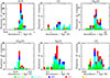 |
Fig. E.1. Same as Fig. 3 for abundances relative to H2O. |
| In the text | |
|
Fig. F.1. Histograms of the sulfur to carbon abundance ratio measured from observations at radio wavelengths. Considered sulfur and carbon-bearing molecules are CO, CH3OH, H2CO, H2S and CS. Only comets for which these five species are detected are considered. Note however that H2CO has a minor abundance, compared to CH3OH and CO, and CS is much less abundant than H2S in most comets. The upper limit for 3I/ATLAS is shown by an orange arrow. See Biver et al. (2024b) and references therein. |
| In the text | |
|
Fig. G.1. Initial velocity V0, maximal velocity Vmax, and terminal velocity for free-molecular expansion Vfree as a function of source temperature (TN). From left to right, CO2-dominated, H2O-dominated, and H2O-CO2 gas mixture. The range for 3I/ATLAS (in blue) delineates the expansion velocities measured in the blue and red wings of the line profiles (i.e. VHM values, see main text). |
| In the text | |
Current usage metrics show cumulative count of Article Views (full-text article views including HTML views, PDF and ePub downloads, according to the available data) and Abstracts Views on Vision4Press platform.
Data correspond to usage on the plateform after 2015. The current usage metrics is available 48-96 hours after online publication and is updated daily on week days.
Initial download of the metrics may take a while.