| Issue |
A&A
Volume 709, May 2026
|
|
|---|---|---|
| Article Number | L9 | |
| Number of page(s) | 8 | |
| Section | Letters to the Editor | |
| DOI | https://doi.org/10.1051/0004-6361/202659271 | |
| Published online | 05 May 2026 | |
Letter to the Editor
Extended coronal line emission and new clues to a possible dual AGN in the merger J1356+1026
1
Instituto de Astrofísica de Canarias, Calle Vía Láctea, s/n, E-38205 La Laguna, Tenerife, Spain
2
Departamento de Astrofísica, Universidad de La Laguna, E-38206 La Laguna, Tenerife, Spain
3
Instituto de Radioastronomía and Astrofísica (IRyA-UNAM), 3-72 (Xangari), 8701 Morelia, Mexico
4
INAF – Osservatorio Astrofisico di Arcetri, Largo E. Fermi 5, 50127 Firenze, Italy
5
Divisão de Astrofísica, INPE, Avenida dos Astronautas 1758, São José dos Campos, 12227-010, SP, Brazil
6
Instituto de Física Fundamental, CSIC, Calle Serrano 123, 28006 Madrid, Spain
7
Department of Physics & Astronomy, University of Sheffield, S3 7RH, Sheffield, UK
8
Centro de Astrobiología (CAB), CSIC-INTA, Camino Bajo del Castillo s/n, E-28692 Villanueva de la Cañada, Madrid, Spain
9
Department of Physics, University of Oxford, Oxford OX1 3RH, UK
10
School of Sciences, European University Cyprus, Diogenes Street, Engomi 1516, Nicosia, Cyprus
11
Telespazio UK for the European Space Agency, ESAC, Camino Bajo del Castillo s/n, 28692 Villanueva de la Cañada, Spain
12
Observatorio Astronómico Nacional (OAN-IGN)-Observatorio de Madrid, Alfonso XII, 3, 28014 Madrid, Spain
★ Corresponding author: This email address is being protected from spambots. You need JavaScript enabled to view it.
Received:
2
February
2026
Accepted:
13
April
2026
Abstract
Merging luminous galaxies are ideal laboratories for studying some of the most extreme astrophysical phenomena. The local (z = 0.1232) obscured quasar J1356+1026 has two nuclei, North and South (J1356N and J1356S), but despite numerous efforts, J1356S had not yet been confirmed as an AGN. Based on the superb sensitivity and spatial resolution of the MIRI/MRS instrument on board the JWST, we present new evidence suggesting that J1356S may indeed host an AGN with log Lbol = 43.4±0.080.50.6 erg s−1. This is supported by the detection of strong coronal line emission at this location and by a spectral shape that differs from that of J1356N and those of the narrow-line region. Aided by the spatially resolved information of MIRI/MRS and VLT/SINFONI, we also found that the high-ionization gas, traced by the coronal lines [Ne V]14.3 μm and [Si VI]1.963 μm, extends from ∼13 − 15.5 kpc. This is likely a lower limit of the true extension, as suggested by the comparison with optical imaging from HST. The extended [Ne V] emission can be accounted for by photoionization from the quasar in J1356N in a relatively low-density environment, ranging from ne ≤ 2000 − 3800 cm−3 in J1356N and ne ≤ 600 − 1200 cm−3 in J1356S and the narrow-line region, as measured from the [Ne V]14.3 μm and 24.3 μm lines.
Key words: ISM: lines and bands / galaxies: active / galaxies: nuclei / quasars: general
© The Authors 2026
 Open Access article, published by EDP Sciences, under the terms of the Creative Commons Attribution License (https://creativecommons.org/licenses/by/4.0), which permits unrestricted use, distribution, and reproduction in any medium, provided the original work is properly cited.
This article is published in open access under the Subscribe to Open model. This email address is being protected from spambots. You need JavaScript enabled to view it. to support open access publication.
1. Introduction
The connection between merging galaxies and active galactic nuclei (AGN) in luminous hosts, oftentimes including an obscured phase, has long been regarded as having a fundamental role in shaping galaxy evolution (e.g. Sanders & Mirabel 1996). In this coevolution scenario, two AGN separated by ≲10 kpc and sharing the same host galaxy (dual AGN) during certain periods of time is a tangible possibility (De Rosa et al. 2019; Koss et al. 2012). Dual AGN are often confirmed using X-ray data (e.g., Komossa et al. 2003) and/or emission line diagnostics obtained via observations with a high spectral and spatial resolution (e.g. U et al. 2013; Koss et al. 2023; Hermosa Muñoz et al. 2025). An example of the latter are coronal lines (Rodríguez-Ardila et al. 2025), whose ionization potentials (IPs) of ≳100 eV make it unlikely that phenomena associated with star formation ionize the atoms at these energies, although a contribution from shocks cannot be discarded (Contini & Viegas 2001; Hernandez et al. 2025).
Type 2 quasars (QSO2s) are dust-obscured type 1 quasars that are frequently found in interacting and/or merging galaxies (Pierce et al. 2023). These targets are thought to represent a crucial transition phase in the evolution of luminous galaxies that occurs between a gas-rich merger and a type 1 quasar phase (Hopkins et al. 2008). A local example of this class of objects is SDSS J135646.10+102609.0, hereafter J1356. It is part of the Quasar Feedback (QSOFEED) sample (Bessiere et al. 2024) and is hosted in a galaxy merger with log (LIR/L⊙) = 11.8 (Greene et al. 2009; Ramos Almeida et al. 2022). It shows a large-scale ionized outflow (Greene et al. 2012) and two stellar nuclei separated by ∼1.31″ (2.9 kpc), as measured from Hubble Space Telescope (HST) F160W imaging (Comerford et al. 2015): the North nucleus, hereafter J1356N, where the QSO2 is located, and the South nucleus, J1356S, candidated to host another AGN.
Using Chandra data, Comerford et al. (2015) measured emission at > 5σ and 4.4σ, which are associated with the position of the two stellar bulges identified in the F160W image. They were unable to confirm J1356S as an AGN, however, because of the surrounding diffuse soft X-ray emission, which is likely associated with the outflow. Deeper Chandra observations were used by Foord et al. (2020) with the same result. J1356N and J1356S were both detected in cold and hot molecular gas (Sun et al. 2014; Ramos Almeida et al. 2022; Zanchettin et al. 2025), but no radio detections of J1356S in sub-arcsecond resolution data have been reported so far (Jarvis et al. 2019; Njeri et al. 2025). Beyond the complex nuclear region, J1356 has a small companion galaxy to the north (∼57 kpc), a ∼20 kpc [O III] expanding bubble to the south (Greene et al. 2012; Speranza et al. 2024), and diffuse X-ray emission (Greene et al. 2014; Foord et al. 2020).
The availability of JWST MIRI/MRS data of J1356, first published by Ramos Almeida et al. (2025, hereafter RA25), allowed us to investigate its possible dual AGN nature and extended coronal line emission by means of several neon lines. We adopted a cosmology of H0 = 70 km s−1 Mpc−1, Ωm = 0.3, and ΩΛ = 0.7. J1356 has a redshift of z = 0.1232, corresponding to a luminosity distance of 575.8 Mpc and a spatial scale of 2.213 kpc/″.
2. Observations and data reduction
The data we analyzed are part of the JWST General Observer program 3655 (PI: Ramos Almeida; MAST doi:10.17909/8w9h-re72), previously published in RA25. The data of J1356 were taken on January 26, 2025, using a four- and two-point dither sequence for the target and background observations, respectively. We refer to RA25 for details on the observations and data reduction. In addition to the standard data reduction, we also used point spread function (PSF) subtracted cubes. The PSF subtraction and associated data reduction were performed as described in González-Martín et al. (2025). This procedure is crucial to remove the contamination from the bright point source associated with J1356N (i.e., the QSO2), and allowed us to study the underlying extended emission (see Fig. 1) and the spectrum of J1356S.
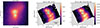 |
Fig. 1. HST/WFC3 F160W image of J1356 in logarithmic scale (left) showing a similar region as the [Ne V] 14.3 μm [−200, 0] km s−1 velocity channel map obtained from the original (center) and PSF-subtracted (right) JWST/MIRI cubes. The zero velocity corresponds to the central wavelength of [Ne V], redshifted to z = 0.1232. The color bar is in units of erg s−1 cm−2. The [Ne V] emission extends to ∼6″ (∼13 kpc) along PA ∼ 30°. The contours correspond to the HST F160W image, where J1356N and J1356S can be clearly identified. The blue and green circles indicate the regions from which the spectra shown in Fig. 2 were extracted. |
3. The dual AGN nature of J1356
Figure 1 shows the HST/WFC3 F160W contours overlaid on the [Ne V]14.3 μm channel maps, showing the position of J1356N and J1356S. We applied the routine find_peaks from Astropy to determine the coordinates of the peak positions on the HST image, which are 1.28″ (2.8 kpc) apart in projection. To extract the MIRI/MRS spectra of the two nuclei, we matched the peak of the local continuum around the [Ne V] line to the position of J1356N in the HST/WFC3 F160W image. From this alignment, we determined the relative position of J1356S in the MIRI/MRS data (at 1.28″ from J1356N). We then used the CAFE Region Extraction Tool Automaton (CRETA, Diaz-Santos et al. 2025) to perform the 1D extractions in circular apertures with a radius of 0.4″ to match the angular resolution of Ch4. Fig. 1 shows the extraction apertures, and Fig. 2 shows the corresponding spectra. The distinct nature of J1356N, whose mid-infrared spectrum was first reported in RA25, and that of J1356S, shown here for the first time, is evident from the different spectral shapes and relative line strengths (see Fig. 2 and Table A.1). The intensities of the coronal lines compared to lower-ionization lines such as [Ne II]12.8 μm and [Ne III]15.5 μm are higher in J1356S1. The 9.7 μm silicate absorption feature is weaker in J1356S, but the polycyclic aromatic hydrocarbons (PAHs) are stronger than in J1356N. In addition, J1356S is clearly detected in H2 (see the bottom panel of Fig. A.2).
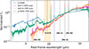 |
Fig. 2. Spectra from J1356N (blue), J1356S (green), and two NLR locations (pink and orange) extracted in circular apertures with a radius of 0.4″ (shown in Fig. A.1), normalized at 15 μm. The spectrum of J1356N was extracted from the original cubes, and the other spectra were extracted from the PSF-subtracted cubes. The spectra of the NLR could only be extracted from Ch2 to Ch4 because the size of the Ch1 FOV is limited. The emission lines we used are labeled. The purple and yellow shaded regions indicate the 6.2 and 11.3 μm PAHs and the 9.7 μm silicate absorption. For reference, the continuum fluxes at 15 μm of J1356N, J1356S, and NLR S and N are 22.1, 1.31, 0.87, and 0.52 mJy. |
Despite the clear differences between J1356N and J1356S spectra, no point source is detected in the MIRI/MRS continuum for J1356S2. The reason might be the contrast (a relatively weak AGN embedded in a bright galaxy merger), but J1356S might also be a stellar nucleus whose mid-infrared spectrum shows projected narrow-line region (NLR) emission from the QSO2 (J1356N). To test this possibility, we extracted spectra in two circular apertures with radii of 0.4″ centered on two locations dominated by the NLR (see Fig. A.1). The NLR emission was identified using the [Ne III]/[Ne II] map, following García-Bernete et al. (2024). The slopes of the NLR spectra (pink and orange lines in Fig. 2) are the same, but they are distinct from J1356N and J1356S. Together with the location of J1356S outside of the two projected ionization cones shown in Fig. A.1, this suggests that it is not just part of the NLR of J1356N.
We measured the total flux of [Ne II], [Ne III], and [Ne V] in J1356N and J1356S, and in the two NLR spectra shown in Fig. 2 (see Table A.1). [Ne V]/[Ne II] is a diagnostic for nuclear activity, with AGN typically showing [Ne V]/[Ne II] > 0.1 (Inami et al. 2013), and [Ne III]/[Ne II] is sensitive to the hardness of the radiation field (Groves et al. 2008). Fig. 3 shows the [Ne V]/[Ne II] versus [Ne III]/[Ne II] diagram, including the models from Feltre et al. (2016, 2023), computed for Lbol = 1045 erg s−1 (see Appendix A for details). The ratios of J1356N, J1356S, and the NLR South (NLR S) are consistent with these AGN photoionization models and with those of the five QSO2s studied in RA25 and the Seyfert galaxies from Zhang et al. (2024). A clear positive trend is followed by all data points, with the NLR spectra of J1356 showing the highest values of both ratios (see Table A.1). We used PyNeb (Luridiana et al. 2015) with Te = 104 and 2 × 10⁴ K, as in RA25, and the [Ne V]14.3/24.3 μm ratio to calculate the electron densities. This resulted in ne ≤ 2000 − 3800 cm−3 for J1356N and ne ≤ 600 − 1200 cm−3 for J1356S and NLR S (see Table A.1). These values are consistent with the range of densities covered by the AGN photoionization models shown in Fig. 3, of 102–104 cm−3. The density decreases with distance from J1356N, with NLR N possibly having ne ≲ 100 cm−3, according to its position in Fig. 3 and low [Ne V]14.3/24.3 μm ratio.
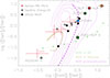 |
Fig. 3. [Ne V]/[Ne II] vs. [Ne III]/[Ne II] diagram. The ratios corresponding to the spectra in Fig. 2 are shown as blue, green, orange, and pink circles. The NLR-subtracted ratios of J1356S are shown as a green square. The black dots show the QSO2s in RA25, the black crosses show the Seyferts from Zhang et al. (2024), and the open diamond shows the North nucleus of the dual AGN NGC 6240 (Hermosa Muñoz et al. 2025). The red lines indicate the median ratios of QSOs, Seyferts, and LINERs from PS10, measured from Spitzer/IRS spectra. The purple contours delineate the full grid of AGN photoionization models from Feltre et al. (2016), and green asterisks and brown diamonds show the AGN+SF and AGN+shocks models from Feltre et al. (2023) (see Appendix A for details). |
Based on the JWST/MIRI observations of J1356S, it is possible that this stellar bulge hosts an AGN with a luminosity lower than that of J1356N, but we cannot securely rule out that it is a star-forming galaxy whose spectrum shows projected emission from the NLR of J1356N. We subtracted the Ne line fluxes measured in the spectrum of NLR S from those of J1356S and plot the resulting ratios in Fig. 3 (green square). The fluxes are consistent with AGN photoionization alone, but also with the AGN+SF model. However, both ratios are still higher than those reported for LINERs in Pereira-Santaella et al. (2010, hereafter PS10). From the NLR-subracted [Ne V]14.3 μm flux of J1356S, we estimate  erg s−1 using Eq. (2) from Spinoglio et al. (2022). For J1356N, we measure log Lbol = 45.4 ± 0.2 erg s−1, which is consistent with the value of 45.3 erg s−1 measured from the extinction-corrected [O III] flux (RA25). Using the rest-frame intrinsic 2−7 keV luminosities reported by Foord et al. (2020) for J1356N and J1356S, and the correction of 20 from Vasudevan & Fabian (2007), we obtain log
  and
and  erg s−1, respectively. The LINERs with log Lbol ≲ 43 erg s−1 in PS10 show lower [Ne V]/[Ne II] and [Ne III]/[Ne II] ratios than the NLR-subtracted J1356S values (see Fig. 3), which means that Lbol estimated from [Ne V] is more likely to be representative of the possible AGN than that from the X-rays.
4. The extended coronal line gas
A visual inspection of the MIRI/MRS data cubes revealed extended emission in the coronal lines, including [Ne V]14.3 μm and [Ne VI]7.7 μm (IPs = 97 and 126 eV). To investigate this further, we built continuum-subtracted velocity channel maps. Fig. 1 shows the original and PSF-subtracted [−200, 0] km s−1 channel map of [Ne V], which show an extended and clumpy gas distribution. These clumpy structures are also observed in the [Ne VI] channel maps (see Fig. A.4), which cover a smaller field of view (FOV) than the [Ne V] maps. The maximum extension measured from the [Ne V] maps along a position angle (PA) of ∼30° is ∼6″ (∼13 kpc).
The bright [Ne V] emission at the southern edge of the FOV (detected at 6σ and 4σ in the original and PSF-subtracted cubes; see Figs. 1 and A.5) suggests that it might extend even farther. A comparison with the HST/WFC3 F438W image of J1356 (see the top panel of Fig. A.6) shows a clear correspondence between the [Ne V] emission contours and the optical emission, mostly dominated by [O II]3726,3728 Å in that filter (see the bottom panel of Fig. A.6 for comparison, dominated by the near-infrared stellar continuum). Further supporting evidence for an even more extended [Ne V] emission comes from the [Si VI]1.963 μm emission shown in the left panel of Fig. A.2, obtained from the VLT/SINFONI data first published by Zanchettin et al. (2025). The [Si VI] emission is detected at 3σ at the southern edge of the SINFONI FOV, with an extension of up to ∼5″ to the south of J1356N and ∼7″ of total extension (∼15.5 kpc). Because the IP of [Si VI] (167 eV) is higher than that of [Ne V], it is reasonable to assume that the [Ne V] has at least the same extension as the [Si VI]-emitting gas. The coronal line emission might even reach the 20 kpc ionized gas outflowing bubble first reported by Greene et al. (2012).
In nearby Seyferts, coronal lines have been observed with extensions ranging from ∼100−200 pc (Riffel et al. 2021) up to ∼2−3 kpc (Rodríguez-Ardila et al. 2025). In local QSO2s, [Si VI] emission extending up to ∼1 kpc has been measured from near-infrared spectra (Ramos Almeida et al. 2017, 2019; Speranza et al. 2022). The maximum extent reported for coronal line emission so far is 23 kpc, measured for the [Fe VII]3760 Å emitting-gas detected in MaNGA data of a galaxy merger at z = 0.13 (Negus et al. 2021). However, [Fe VII] is not detected in the nucleus, making it a good candidate for relic extended coronal emission. Thus, the projected size of the coronal emission of J1356, 13−15.5 kpc, is one the largest ever observed sizes.
To test whether shocks are required to explain the extended coronal emission in J1356 (see Fonseca-Faria et al. 2023; Kader et al. 2026), we calculated the [Ne V]/[Ne II] and [Ne III]/[Ne II] ratios across the whole FOV of Ch3 and plot them in Fig. A.7, together with the same models as in Fig. 3. We can reproduce the extended coronal emission with photoionization from an AGN with the luminosity of J1356N in a relatively low-density environment.
5. Conclusions
In this Letter, we reported the finding of one of the most extended coronal line regions ever detected, traced by [Ne V]14.3 μm and [Si VI]1.963 μm, in the galaxy J1356, reaching a projected extent of 13−15.5 kpc. This extent is likely a lower limit of the true size of the coronal line region, set by the reduced FOV of MIRI/MRS. The large extension can be explained by photoionization from the quasar in J1356N and the relatively low density of the system: ne ≤ 2000 − 3800 cm−3 in J1356N, ne ≤ 600 − 1200 cm−3 in J1356S and NLR S, and possibly a lower density in NLR N.
We also reported new evidence for the possible presence of an AGN with  erg s−1 in J1356S, although we cannot rule out that it is a star-forming galaxy whose mid-infrared spectrum includes projected emission from the NLR of J1356N. Further comparison with low-luminosity AGN and stellar photoionization models, coupled with adaptive optics near-infrared IFU observations, might be required to confirm a dual AGN in this merger system.
Acknowledgments
This work is based on observations made with the NASA/ESA/CSA James Webb Space Telescope. The data were obtained from the Mikulski Archive for Space Telescopes at the Space Telescope Science Institute, which is operated by the Association of Universities for Research in Astronomy, Inc., under NASA contract NAS 5-03127 for JWST and from the European JWST archive (eJWST) operated by the ESAC Science Data Centre (ESDC) of the European Space Agency. MB acknowledges support from the Juan de La Cierva scholarship with reference JDC2023-052684-I, funded by MICIU/AEI/10.13039/501100011033 and FSE+. MB, CRA and AA thank the Agencia Estatal de Investigación of the Ministerio de Ciencia, Innovación y Universidades (MCIU/AEI) under the grant “Tracking active galactic nuclei feedback from parsec to kiloparsec scales”, with reference PID2022−141105NB−I00 and the European Regional Development Fund (ERDF). OG-M acknowledges financial support from the SECIHTI project Ciencia de Frontera CF-2023-G100, UNAM/DGAPA project PAPIIT IN109123, and Estancias Sabáticas PASPA of UNAM/DGAPA. MVZ acknowledges the support from project “VLT-MOONS” CRAM 1.05.03.07. MC thanks the financial support from Coordenação de Aperfeiçoamento de Pessoal de Nível Superior – Brasil (CAPES) – Finance Code 001. IGB is supported by the Programa Atraccíon de Talento Investigador “Cesar Nombela” via grant 2023-T1/TEC-29030 funded by the Community of Madrid. MPS acknowledges support from grants RYC2021-033094-I, CNS2023-145506, and PID2023-146667NB-I00 funded by MCIN/AEI/10.13039/501100011033 and the European Union NextGenerationEU/PRTR. AA is funded by the European Union (Widening Participation, ExGal-Twin, GA 101158446). This work made use of Astropy: a community-developed core Python package and an ecosystem of tools and resources for astronomy (Astropy Collaboration 2018). We thank the anonymous referee for constructive comments that helped improving this manuscript.
References
- Astropy Collaboration (Price-Whelan, A. M., et al.) 2018, AJ, 156, 123 [Google Scholar]
- Bessiere, P. S., Ramos Almeida, C., Holden, L. R., Tadhunter, C. N., & Canalizo, G. 2024, A&A, 689, A271 [NASA ADS] [CrossRef] [EDP Sciences] [Google Scholar]
- Comerford, J. M., Pooley, D., Barrows, R. S., et al. 2015, ApJ, 806, 219 [Google Scholar]
- Contini, M., & Viegas, S. M. 2001, ApJS, 132, 211 [NASA ADS] [CrossRef] [Google Scholar]
- De Rosa, A., Vignali, C., Bogdanović, T., et al. 2019, New Astron. Rev., 86, 101525 [Google Scholar]
- Diaz-Santos, T., Lai, T. S. Y., Finnerty, L., et al. 2025, Astrophysics Source Code Library [record ascl:2501.001] [Google Scholar]
- Feltre, A., Charlot, S., & Gutkin, J. 2016, MNRAS, 456, 3354 [Google Scholar]
- Feltre, A., Gruppioni, C., Marchetti, L., et al. 2023, A&A, 675, A74 [NASA ADS] [CrossRef] [EDP Sciences] [Google Scholar]
- Ferland, G. J., Kisielius, R., Keenan, F. P., et al. 2013, ApJ, 767, 123 [NASA ADS] [CrossRef] [Google Scholar]
- Fonseca-Faria, M. A., Rodríguez-Ardila, A., Contini, M., Dahmer-Hahn, L. G., & Morganti, R. 2023, MNRAS, 524, 143 [CrossRef] [Google Scholar]
- Foord, A., Gültekin, K., Nevin, R., et al. 2020, ApJ, 892, 29 [NASA ADS] [CrossRef] [Google Scholar]
- García-Bernete, I., Rigopoulou, D., Donnan, F. R., et al. 2024, A&A, 691, A162 [NASA ADS] [CrossRef] [EDP Sciences] [Google Scholar]
- González-Martín, O., Díaz-González, D. J., Martínez-Paredes, M., et al. 2025, MNRAS, 539, 2158 [Google Scholar]
- Greene, J. E., Zakamska, N. L., Liu, X., Barth, A. J., & Ho, L. C. 2009, ApJ, 702, 441 [NASA ADS] [CrossRef] [Google Scholar]
- Greene, J. E., Zakamska, N. L., & Smith, P. S. 2012, ApJ, 746, 86 [Google Scholar]
- Greene, J. E., Pooley, D., Zakamska, N. L., Comerford, J. M., & Sun, A.-L. 2014, ApJ, 788, 54 [NASA ADS] [CrossRef] [Google Scholar]
- Groves, B., Nefs, B., & Brandl, B. 2008, MNRAS, 391, L113 [NASA ADS] [Google Scholar]
- Gutkin, J., Charlot, S., & Bruzual, G. 2016, MNRAS, 462, 1757 [Google Scholar]
- Hermosa Muñoz, L., Alonso-Herrero, A., Labiano, A., et al. 2025, A&A, 693, A321 [NASA ADS] [CrossRef] [EDP Sciences] [Google Scholar]
- Hernandez, S., Smith, L. J., Jones, L. H., et al. 2025, ApJ, 983, 154 [Google Scholar]
- Hopkins, P. F., Hernquist, L., Cox, T. J., & Kereš, D. 2008, ApJS, 175, 356 [Google Scholar]
- Inami, H., Armus, L., Charmandaris, V., et al. 2013, ApJ, 777, 156 [Google Scholar]
- Jarvis, M. E., Harrison, C. M., Thomson, A. P., et al. 2019, MNRAS, 485, 2710 [Google Scholar]
- Kader, J. A., U, V., Barcos-Muñoz, L., et al. 2026, Science, 391, 911 [Google Scholar]
- Komossa, S., Burwitz, V., Hasinger, G., et al. 2003, ApJ, 582, L15 [NASA ADS] [CrossRef] [Google Scholar]
- Koss, M., Mushotzky, R., Treister, E., et al. 2012, ApJ, 746, L22 [Google Scholar]
- Koss, M. J., Treister, E., Kakkad, D., et al. 2023, ApJ, 942, L24 [Google Scholar]
- Luridiana, V., Morisset, C., & Shaw, R. A. 2015, A&A, 573, A42 [NASA ADS] [CrossRef] [EDP Sciences] [Google Scholar]
- Negus, J., Comerford, J. M., Müller Sánchez, F., et al. 2021, ApJ, 920, 62 [NASA ADS] [CrossRef] [Google Scholar]
- Njeri, A., Harrison, C. M., Kharb, P., et al. 2025, MNRAS, 537, 705 [Google Scholar]
- Pereira-Santaella, M., Diamond-Stanic, A. M., Alonso-Herrero, A., & Rieke, G. H. 2010, ApJ, 725, 2270 [Google Scholar]
- Pierce, J. C. S., Tadhunter, C., Ramos Almeida, C., et al. 2023, MNRAS, 522, 1736 [NASA ADS] [CrossRef] [Google Scholar]
- Ramos Almeida, C., Piqueras López, J., Villar-Martín, M., & Bessiere, P. S. 2017, MNRAS, 470, 964 [NASA ADS] [CrossRef] [Google Scholar]
- Ramos Almeida, C., Acosta-Pulido, J. A., Tadhunter, C. N., et al. 2019, MNRAS, 487, L18 [NASA ADS] [CrossRef] [Google Scholar]
- Ramos Almeida, C., Bischetti, M., García-Burillo, S., et al. 2022, A&A, 658, A155 [NASA ADS] [CrossRef] [EDP Sciences] [Google Scholar]
- Ramos Almeida, C., García-Bernete, I., Pereira-Santaella, M., et al. 2025, A&A, 698, A194 [NASA ADS] [CrossRef] [EDP Sciences] [Google Scholar]
- Riffel, R. A., Bianchin, M., Riffel, R., et al. 2021, MNRAS, 503, 5161 [NASA ADS] [CrossRef] [Google Scholar]
- Rodríguez-Ardila, A., Fonseca-Faria, M. A., Dahmer-Hahn, L. G., et al. 2025, MNRAS, 538, 2800 [Google Scholar]
- Sanders, D. B., & Mirabel, I. F. 1996, ARA&A, 34, 749 [Google Scholar]
- Speranza, G., Ramos Almeida, C., Acosta-Pulido, J. A., et al. 2022, A&A, 665, A55 [NASA ADS] [CrossRef] [EDP Sciences] [Google Scholar]
- Speranza, G., Ramos Almeida, C., Acosta-Pulido, J. A., et al. 2024, A&A, 681, A63 [NASA ADS] [CrossRef] [EDP Sciences] [Google Scholar]
- Spinoglio, L., Fernández-Ontiveros, J. A., & Malkan, M. A. 2022, ApJ, 941, 46 [NASA ADS] [CrossRef] [Google Scholar]
- Sun, A.-L., Greene, J. E., Zakamska, N. L., & Nesvadba, N. P. H. 2014, ApJ, 790, 160 [NASA ADS] [CrossRef] [Google Scholar]
- U, V., Medling, A., Sanders, D., et al. 2013, ApJ, 775, 115 [Google Scholar]
- Vasudevan, R. V., & Fabian, A. C. 2007, MNRAS, 381, 1235 [NASA ADS] [CrossRef] [Google Scholar]
- Zanchettin, M. V., Ramos Almeida, C., Audibert, A., et al. 2025, A&A, 695, A185 [NASA ADS] [CrossRef] [EDP Sciences] [Google Scholar]
- Zhang, L., Packham, C., Hicks, E. K. S., et al. 2024, ApJ, 974, 195 [NASA ADS] [CrossRef] [Google Scholar]
The K-band spectra of J1356N and J1356S, shown in Fig. 1 in Zanchettin et al. (2025), also show different slopes and [Si VI] emission.
The PSF-subtracted cubes show mid-infrared continuum emission from J1356S (see Fig. A.3), which is also detected in the near-infrared (HST/WFC3 and VLT/SINFONI).
Appendix A: Supporting material
This Appendix provides supporting evidence for the possible dual AGN nature and extended coronal line emission of J1356.
The models shown as purple lines in Fig. 3 correspond to the grid of photoionization models of AGN NLR from Feltre et al. (2016), which were computed using the CLOUDY code (version c13.03; Ferland et al. 2013) and the same parametrization of the metal and dust content in the ionized gas as in Gutkin et al. (2016). Feltre et al. (2016) chose an open geometry and a broken power law of spectral index α ranging from -2 to -1.2 to reproduce the emission from the AGN accretion disc, which is described in Eq. 5 there. They adopted a fixed AGN luminosity of 1045 erg s−1 cm−2, an inner radius of the NLR of 300 pc, ionization parameter (U) in the range −4 ≤ log U ≤ −1, fifteen values of the metallicity in the range 0.0001 ≤ Z ≤ 0.07, and dust-to-metal mass ratios in the range 0.1 ≤ ξd ≤ 0.5. Finally, they considered hydrogen number densities (nH) ranging from 100 to 10 000 cm−3, which are consistent with the electron densities measured from the [Ne V] lines except in the case of NLR N, where it is lower (see Table A.1). The purple dashed line in Fig. 3 correspond to the photoionization model with nH = 103 cm−3 (in good agreement with the electron density measured from the [Ne V] line, of ∼1300 cm−3), Z = 0.017, ξd = 0.3, α = 0.7, and log(⟨U⟩) varying from -1.5 to -4.5 from top to bottom. The green asterisks and brown diamonds are the AGN+star formation (SF) and AGN+shocks models from Feltre et al. (2023). They have 90% contribution to the total Hβ emission from star formation and shocks, respectively. In the case of the SF+AGN model, the ionization parameter increases from log(⟨U⟩) = -3.0 from left to right. While in the AGN+shocks model, the shock velocity goes from 200 to 1000 km s−1 counterclockwise from bottom to top.
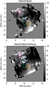 |
Fig. A.1. [Ne III]15.5μm/[Ne II]12.8μm emission line ratio measured from the original (top) and PSF-subtracted (bottom) cubes. The extractions corresponding to J1356N, J1356S, and the two locations within the ionization cones (NLR N and NLR S) are indicated as blue, green, pink, and orange circles. |
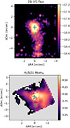 |
Fig. A.2. The top panel shows the VLT/SINFONI continuum-subtracted [Si VI]1.963 μm flux map obtained from the fitting of one Gaussian component to the emission line. The color bar is in units of erg s−1 cm−2. The bottom panel shows the JWST/MIRI PSF- and continuum-subtracted H20 − 0S(3) moment 0 map, with the color bar in units of mJy sr−1 km s−1. The crosses indicate the position of the J1356N and J1356S. The South nucleus coincides with a clump of H2. An in-depth analysis of the H2 excitation and kinematics will be presented in Zanchettin et al. (in prep.). |
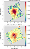 |
Fig. A.3. Local continuum centered at 5.9 μm in the original (top) and PSF-subtracted (bottom) cubes. The black contours correspond to the HST/WFC3 F160W image and indicate the location of J1356N and J1356S. |
 |
Fig. A.4. [Ne VI]7.6μm velocity channel maps from -1400 to 1000 km s−1 in increments of 400 km s−1. The velocity slice used to produce each channel map is indicated on the top left corner of each panel. The zero velocity corresponds to the central wavelength of [Ne V], redshifted to z = 0.1232. The local continuum in each spaxel, modeled by a first degree polynomial, is subtracted from the line flux before building the velocity channels. The color bar is in logarithmic scale in units of erg s−1 cm−2 pix−1. The VLA 6 GHz contours from Jarvis et al. (2019) are overlaid, at levels of (3, 10, 15, 30, 60)×σ. The stars mark the location of J1356N and J1356S measured from the HST F160W image (see Fig. 1). |
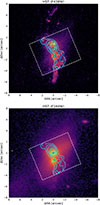 |
Fig. A.6. HST/WFC3 F438W and F160W images with the MIRI/MRS [Ne V] flux contours overlaid in cyan. The dashed white box indicates the size of the MRS Ch3 FOV, and the crosses mark the position of J1356N and J1356S. |
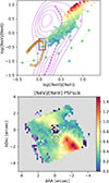 |
Fig. A.7. Same as Fig. 3 for the spatially resolved measurements obtained from the PSF-subtracted cubes. The points are color-coded according to the [Ne V]/[Ne III] line ratio shown in the bottom panel. The purple box (0 < log([Ne III]/[Ne II]) < 0.15 and −0.6 < log([Ne V]/[Ne II]) < − 0.2) indicates the points closer to the AGN+shocks models (brown diamonds). Their spatial location is indicated by the purple areas on the bottom panel. |
Emission line fluxes of [Ne II], [Ne III], and [Ne V] and corresponding ratios
All Tables
Emission line fluxes of [Ne II], [Ne III], and [Ne V] and corresponding ratios
All Figures
|
Fig. 1. HST/WFC3 F160W image of J1356 in logarithmic scale (left) showing a similar region as the [Ne V] 14.3 μm [−200, 0] km s−1 velocity channel map obtained from the original (center) and PSF-subtracted (right) JWST/MIRI cubes. The zero velocity corresponds to the central wavelength of [Ne V], redshifted to z = 0.1232. The color bar is in units of erg s−1 cm−2. The [Ne V] emission extends to ∼6″ (∼13 kpc) along PA ∼ 30°. The contours correspond to the HST F160W image, where J1356N and J1356S can be clearly identified. The blue and green circles indicate the regions from which the spectra shown in Fig. 2 were extracted. |
| In the text | |
|
Fig. 2. Spectra from J1356N (blue), J1356S (green), and two NLR locations (pink and orange) extracted in circular apertures with a radius of 0.4″ (shown in Fig. A.1), normalized at 15 μm. The spectrum of J1356N was extracted from the original cubes, and the other spectra were extracted from the PSF-subtracted cubes. The spectra of the NLR could only be extracted from Ch2 to Ch4 because the size of the Ch1 FOV is limited. The emission lines we used are labeled. The purple and yellow shaded regions indicate the 6.2 and 11.3 μm PAHs and the 9.7 μm silicate absorption. For reference, the continuum fluxes at 15 μm of J1356N, J1356S, and NLR S and N are 22.1, 1.31, 0.87, and 0.52 mJy. |
| In the text | |
|
Fig. 3. [Ne V]/[Ne II] vs. [Ne III]/[Ne II] diagram. The ratios corresponding to the spectra in Fig. 2 are shown as blue, green, orange, and pink circles. The NLR-subtracted ratios of J1356S are shown as a green square. The black dots show the QSO2s in RA25, the black crosses show the Seyferts from Zhang et al. (2024), and the open diamond shows the North nucleus of the dual AGN NGC 6240 (Hermosa Muñoz et al. 2025). The red lines indicate the median ratios of QSOs, Seyferts, and LINERs from PS10, measured from Spitzer/IRS spectra. The purple contours delineate the full grid of AGN photoionization models from Feltre et al. (2016), and green asterisks and brown diamonds show the AGN+SF and AGN+shocks models from Feltre et al. (2023) (see Appendix A for details). |
| In the text | |
|
Fig. A.1. [Ne III]15.5μm/[Ne II]12.8μm emission line ratio measured from the original (top) and PSF-subtracted (bottom) cubes. The extractions corresponding to J1356N, J1356S, and the two locations within the ionization cones (NLR N and NLR S) are indicated as blue, green, pink, and orange circles. |
| In the text | |
|
Fig. A.2. The top panel shows the VLT/SINFONI continuum-subtracted [Si VI]1.963 μm flux map obtained from the fitting of one Gaussian component to the emission line. The color bar is in units of erg s−1 cm−2. The bottom panel shows the JWST/MIRI PSF- and continuum-subtracted H20 − 0S(3) moment 0 map, with the color bar in units of mJy sr−1 km s−1. The crosses indicate the position of the J1356N and J1356S. The South nucleus coincides with a clump of H2. An in-depth analysis of the H2 excitation and kinematics will be presented in Zanchettin et al. (in prep.). |
| In the text | |
|
Fig. A.3. Local continuum centered at 5.9 μm in the original (top) and PSF-subtracted (bottom) cubes. The black contours correspond to the HST/WFC3 F160W image and indicate the location of J1356N and J1356S. |
| In the text | |
|
Fig. A.4. [Ne VI]7.6μm velocity channel maps from -1400 to 1000 km s−1 in increments of 400 km s−1. The velocity slice used to produce each channel map is indicated on the top left corner of each panel. The zero velocity corresponds to the central wavelength of [Ne V], redshifted to z = 0.1232. The local continuum in each spaxel, modeled by a first degree polynomial, is subtracted from the line flux before building the velocity channels. The color bar is in logarithmic scale in units of erg s−1 cm−2 pix−1. The VLA 6 GHz contours from Jarvis et al. (2019) are overlaid, at levels of (3, 10, 15, 30, 60)×σ. The stars mark the location of J1356N and J1356S measured from the HST F160W image (see Fig. 1). |
| In the text | |
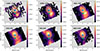 |
Fig. A.5. Same as Fig. A.4, but for the [Ne V]14.3μm emission. |
| In the text | |
|
Fig. A.6. HST/WFC3 F438W and F160W images with the MIRI/MRS [Ne V] flux contours overlaid in cyan. The dashed white box indicates the size of the MRS Ch3 FOV, and the crosses mark the position of J1356N and J1356S. |
| In the text | |
|
Fig. A.7. Same as Fig. 3 for the spatially resolved measurements obtained from the PSF-subtracted cubes. The points are color-coded according to the [Ne V]/[Ne III] line ratio shown in the bottom panel. The purple box (0 < log([Ne III]/[Ne II]) < 0.15 and −0.6 < log([Ne V]/[Ne II]) < − 0.2) indicates the points closer to the AGN+shocks models (brown diamonds). Their spatial location is indicated by the purple areas on the bottom panel. |
| In the text | |
Current usage metrics show cumulative count of Article Views (full-text article views including HTML views, PDF and ePub downloads, according to the available data) and Abstracts Views on Vision4Press platform.
Data correspond to usage on the plateform after 2015. The current usage metrics is available 48-96 hours after online publication and is updated daily on week days.
Initial download of the metrics may take a while.