


| Issue |
A&A
Volume 711, July 2026
|
|
|---|---|---|
| Article Number | A262 | |
| Number of page(s) | 13 | |
| Section | Stellar structure and evolution | |
| DOI | https://doi.org/10.1051/0004-6361/202659151 | |
| Published online | 21 July 2026 | |
SN 2024igg: A super-Chandrasekhar/03fg-like supernova exhibiting C II-dominated spectra after explosion
1
Department of Physics, Tsinghua University, Beijing 100084, China
2
Department of Astronomy, University of California, Berkeley CA 94720-3411, USA
3
INAF – Osservatorio Astronomico di Padova, Vicolo dell’Osservatorio 5 35122 Padova, Italy
4
Università degli Studi di Padova, Dipartimento di Fisica e Astronomia, Vicolo dell’Osservatorio 2 35122 Padova, Italy
5
Centro di Ateneo di Studi e Attività Spaziali “Giuseppe Colombo”, Via Venezia 1, I-35131 Padova, Italy
6
INFN – Sezione di Padova, Via Marzolo 8, I-35131 Padova, Italy
7
INAF – Osservatorio Astronomico di Brera, Via Bianchi 46, 23807 Merate (LC), Italy
8
Yunnan Observatories, Chinese Academy of Sciences, Kunming 650216, China
9
International Centre of Supernovae, Yunnan Key Laboratory, Kunming 650216, China
10
Key Laboratory for the Structure and Evolution of Celestial Objects, Chinese Academy of Sciences, Kunming 650216, China
11
School of Astronomy and Space Science, University of Chinese Academy of Sciences, Beijing 100049, China
12
Institute of Astrophysics, Central China Normal University, Wuhan 430079, China
13
Education Research and Application Center, National Astronomical Data Center, Wuhan 430079, China
14
Key Laboratory of Quark and Lepton Physics (Central China Normal University), Ministry of Education, Wuhan 430079, China
★ Corresponding authors: This email address is being protected from spambots. You need JavaScript enabled to view it.
; This email address is being protected from spambots. You need JavaScript enabled to view it.
Received:
27
January
2026
Accepted:
2
June
2026
Abstract
Aims. We present and analyze photometric and spectroscopic observations of the Type Ia supernova (SN Ia) 2024igg, another super-Chandrasekhar (or 03fg-like) SN whose strong C IIλ6580 feature was initially misidentified as Hα, thereby constraining its progenitor system, explosion parameters, and physical scenario.
Methods. We conducted a comparative analysis of SN 2024igg and other 03fg-like SNe. The radiative-transfer code TARDIS was run to identify the features in the first spectrum at t ≈ −13.9 days. A pseudo-bolometric light curve was constructed using ultraviolet and optical photometry and was then modeled with fitting tools.
Results. SN 2024igg shows many characteristics in common with other 03fg-like objects, such as high ultraviolet flux, slowly declining light curves (Δm15(B) = 0.90 ± 0.08 mag), low expansion velocities, and strong and persistent C II absorption. On the other hand, it exhibits some remarkable properties within this subgroup, including a moderately low optical luminosity (Mmax(B) = − 18.99 ± 0.15 mag), a rise time shorter than 18.5 days, and the strongest C IIλ6580 ever detected. The bolometric analysis yields a 56Ni mass of MNi = 0.547 ± 0.082 M⊙ and an ejecta mass of 1.54+0.22−0.19 M⊙, which marginally exceeds the Chandrasekhar mass. Our TARDIS result indicates that most of the features in the earliest spectrum might be attributed to C II, which is consistent with a model in which an SN explodes within a carbon-rich circumstellar medium (CSM). The CSM interaction would produce a density peak in the ejecta, offering a natural explanation for the slowly evolving line velocities near −8000 km s−1. The CSM may stem from the debris of a secondary white dwarf in a white dwarf merger or the envelope of an asymptotic giant branch star. Combined with the unshifted forbidden lines in the spectrum taken at t ≈ +135 days, we suggest that SN 2024igg comes from a symmetric explosion on a secular timescale after the merger.
Key words: supernovae: general / supernovae: individual: SN 2024igg
© The Authors 2026
 Open Access article, published by EDP Sciences, under the terms of the Creative Commons Attribution License (https://creativecommons.org/licenses/by/4.0), which permits unrestricted use, distribution, and reproduction in any medium, provided the original work is properly cited.
This article is published in open access under the Subscribe to Open model. This email address is being protected from spambots. You need JavaScript enabled to view it. to support open access publication.
1. Introduction
It is widely accepted that Type Ia supernovae (SNe Ia; see, e.g., Filippenko 1997) for a review of the SN classification) originate from thermonuclear explosions of carbon-oxygen (C/O) white dwarfs (WDs; Nomoto et al. 1997; Hillebrandt & Niemeyer 2000). Normal SNe Ia, which adhere to the width-luminosity relation (WLR; also dubbed the Lira-Phillips relation; Phillips 1993; Phillips et al. 1999), serve as vital standardizable candles for measuring the distances to their host galaxies and have played a critical role in revealing the accelerating expansion of the Universe (Riess et al. 1998; Perlmutter et al. 1999), although their progenitor systems and explosion mechanisms remain debated. In recent years, a growing number of peculiar SNe Ia that deviate from the WLR have been observed (Taubenberger 2017), offering new opportunities to probe the final stage of stellar evolution and the physics of thermonuclear explosions.
Super-Chandrasekhar-mass (super-MCh) SNe are a peculiar subclass of SNe Ia. The moniker for this subclass comes from the super-MCh WD progenitor inferred from the light curve of the prototype SN 2003fg (Howell et al. 2006). Specifically, powering the overluminous and broad light curve of SN 2003fg requires a 56Ni mass of ∼1.3 M⊙. This value is already close to MCh (1.4 M⊙), and it thus implies a super-MCh explosion, since even the pure detonation of an MCh WD can produce only 0.92 M⊙ of 56Ni (Khokhlov et al. 1993). As the sample grows, SNe Ia of this subclass are also found to be characterized by a broad light curve, blue ultraviolet (UV) through optical colors, a weak or no i-band secondary maximum, moderately low ejecta velocities, and strong and persistent C II absorption (Taubenberger 2017).
On the other hand, some SNe in common with these characteristics are found to have a comparatively moderate luminosity, similar to (e.g., SN 2012dn; Chakradhari et al. 2014) or even fainter than (e.g., ASASSN-15hy; Lu et al. 2021), a normal SN Ia with the same light-curve width. An explosion of a super-MCh WD seems unnecessary for these moderate SNe, and thus, we follow the moniker of 03fg-like proposed by Ashall et al. (2021) for this subclass hereafter. An interaction of SN ejecta and a carbon-rich circumstellar medium (CSM), which might originate from debris of a double WD merger (Yoon et al. 2007) or the envelope of an asymptotic giant branch (AGB) star, has been included to interpret the common features of 03fg-like SNe in many studies (e.g., Taubenberger et al. 2013; Lu et al. 2021; Ashall et al. 2021; Dimitriadis et al. 2022, 2023; Siebert et al. 2024), since it can increase the total ejecta mass, enrich the carbon abundance, possibly power the light curve, and slow down the ejecta velocity (Noebauer et al. 2016). To verify this scenario, an extremely early-time spectrum would be highly valuable, as the interaction could cause the spectrum to be temporarily dominated by carbon and oxygen lines when the photosphere resides in the C/O-rich shell (Maeda et al. 2023). Spectroscopic observations within days of explosion are available for only a handful of 03fg-like SNe, however, of which only SN 2020esm (Dimitriadis et al. 2022) exhibits a spectrum that can be well fit with just carbon and oxygen lines.
Recently, another 03fg-like object with an early-time spectrum dominated by C II was discovered: SN 2024igg. We present optical photometric and spectroscopic observations of it. The discovery and our observations are described in Section 2. In Section 3 we present the photometric and spectroscopic evolution of this SN and compare it with other well-observed SNe Ia. We also analyze the first spectrum, alongside fits to the pseudo-bolometric light curve. Evidence of CSM interaction and its origin are discussed in Section 4. We summarize our findings in Section 5.
2. Observations and data reduction
2.1. Discovery
SN 2024igg was discovered (Munoz-Arancibia et al. 2024) on 2024 May 7.30 (UTC dates are used throughout this paper; modified Julian date, MJD 60437.30) by the Zwicky Transient Facility (ZTF) at α = 15h09m30.910s, δ = 54° 30′20.24″ (J2000). The last non-detection reported by Munoz-Arancibia et al. (2024) was on MJD 60437.26, just ∼0.04 d before the first detection. The forced photometry provided by Lasair1 turned the non-detections on MJD 60437.26 and MJD 60436.45 into detections, however, yielding a last non-detection on MJD 60433.41 to a limit of 20.86 mag and a first detection of 19.10 mag on MJD 60436.45, both in the ZTF r band. We adopt the Lasair results. The ATLAS o band has a non-detection on MJD 60435.44, but the limit is only 18.74 mag.
In Figure 1 we present an 11.9′×11.9′ color-composite (B/V/r) image, taken with the 0.8 m Tsinghua University–NAOC telescope (TNT; Wang et al. 2008; Huang et al. 2012), of SN 2024igg and nearby field stars. The zoomed-in view shows that the projected location of SN 2024igg is close to the center of the host galaxy NGC 5876, a barred spiral at a redshift of z = 0.01085 (value from the NASA/IPAC Extragalactic Database, NED2). Originally identified as a Type II SN by Meissner et al. (2024) based on a spectrum obtained with the Nordic Optical Telescope (NOT), this object was reclassified as an 03fg-like Type Ia SN by Srivastav et al. (2024) based on the identifications of C II and Si II lines in their spectrum taken with the 2 m Liverpool Telescope (LT; Steele et al. 2004).
 |
Fig. 1. TNT 12′×12′ color-composite (B/V/r) image of SN 2024igg and its host galaxy. The reference stars used to calibrate the photometry are marked with circles. The inset shows the zoomed-in region of the SN (indicated with magenta lines) and its host taken on 2024 June 16. |
2.2. Photometry
We performed photometry of SN 2024igg in the griBV filters with the 0.8 m TNT at Xinglong Station of NAOC, the Lijiang 2.4 m telescope (LJT; Fan et al. 2015) of the Yunnan Observatories, and the Schmidt 67/91 cm Telescope (ST-67/91) of the Osservatorio Astronomico di Asiago. All of these images were preprocessed with bias subtraction and flat-field correction. Since the SN is seriously contaminated by the host-galaxy bulge, we performed template subtraction using HOTPANTS (Becker 2015). For TNT, the templates were obtained on 2025 May 27, about 231 days after the last observation. At a light-curve decline rate of 0.01 mag d−1 due to 56Co decay, the SN flux in the templates would be ∼12% of that at the last observation, corresponding to a systematic error of ∼0.13 mag. For the penultimate observation, which preceded the final observation by 80 days, the systematic error reduces to ∼5%. This estimation should be considered an upper limit, as the actual decline rate is typically higher than 0.01 mag d−1 owing to gamma-ray leakage. The templates for ST-67/91 were obtained on 2025 August 30 (i) and 2025 September 17 (g and r), yielding a systematic error of ≲0.04 mag for the final observation. For the LJT images, we performed the subtraction using the TNT templates, and the corresponding systematic error of the last observation is ≲7%. Then, we applied aperture photometry with the automated photometry of transients pipeline (AUTOPHOT; Brennan & Fraser 2022) for the local reference stars and the template-subtracted SN. The aperture correction was derived from the local reference stars and applied to the SN photometry. The instrumental magnitudes were calibrated against Gaia synthetic photometry (Gaia Collaboration 2023).
SN 2024igg was also observed by the Ultraviolet/Optical Telescope (UVOT; Gehrels et al. 2004; Roming et al. 2005) on board the Neil Gehrels Swift Observatory (Gehrels et al. 2004) in three UV (UVW2, UVM2, and UVW1) and three optical (U, B, and V) filters. We extracted Swift photometry using SWIFT_HOST_SUBTRACTION (Brown et al. 2009, 2014) with the latest Swift calibration database3. On the UVOT templates taken on 2025 June 9, the host flux subtraction was applied to remove the contamination from the host galaxy. Based on the above estimates, the systematic error due to the residual SN flux is ≲5% for the final observation. In addition, we included the g- and r-band photometry of ZTF provided by Lasair.
2.3. Spectroscopy
Optical spectra of SN 2024igg were collected with different instruments, including the Beijing-Faint Object Spectrograph and Camera (BFOSC) mounted on the Xinglong 2.16 m telescope (XLT; Zhang et al. 2016a), the Yunnan Faint Object Spectrograph and Camera (YFOSC) on the LJT, the Asiago Faint Objects Spectrograph and Camera (AFOSC) on the Copernico Telescope on Mount Ekar, the Boller & Chivens spectrograph (B&C) on the Galileo Telescope at Osservatorio Astrofisico di Asiago, the Low Resolution Imaging Spectrometer (LRIS; Oke et al. 1995) on the 10 m Keck-I telescope on Maunakea, the Kast double spectrograph (Miller & Stone 1993) on the 3 m Shane telescope at Lick Observatory, and the Low Resolution Spectrograph (LRS) on Telescopio Nazionale Galileo (TNG) on the island of La Palma. Standard IRAF4 routines were used to reduce all the spectra except for the Keck I/LRIS spectrum, which was reduced using the LPIPE pipeline (Perley 2019). Flux calibration of the spectra was performed with spectrophotometric standard stars observed on the same nights. Atmospheric extinction was corrected with the extinction curves of local observatories. We derived the telluric correction using the spectrophotometric standard star. To minimize differential slit losses, LRIS has an atmospheric-dispersion corrector (Filippenko 1982), and all other spectra were observed at the parallactic angle, with the exception of those obtained using BFOSC and YFOSC. The spectra from these two instruments at airmass > 1.2 may therefore have differential slit losses. In addition, we included the two spectra mentioned in Section 2.1. All of the photometry and the journal of spectroscopic observations of SN 2024igg are presented in Appendix A.
3. Analysis
3.1. Reddening and distance
The Galactic reddening on the line of sight is E(B − V)Gal = 0.011 mag (Schlafly & Finkbeiner 2011). No obvious interstellar Na I D absorption at the host redshift is seen in the spectra of SN 2024igg, although the projected distance of the SN to its host-galaxy center is small. We therefore adopted a reddening of E(B − V) = 0.011 mag and a Fitzpatrick (1999) reddening law with RV = 3.1 in this work. The sole redshift-independent distance estimate for NGC 5876 comes from the Tully-Fisher relation, yielding a distance modulus of 34.08 ± 0.46 mag (Theureau et al. 2007) with a large uncertainty. We used the cosmological distance because the redshift of NGC 5876 is ≳0.01. Adopting H0 = 73 ± 5 km s−1 Mpc−1 (the value was taken from Riess et al. 2022, and the uncertainty considers the Hubble tension) and correcting for peculiar motions related to the Virgo cluster and Great Attractor (Mould et al. 2000), we estimate the distance to NGC 5876 to be 51.2 ± 3.5 Mpc. This corresponds to a distance modulus of 33.55 ± 0.15 mag.
3.2. Photometric evolution
Figure 2 shows all the light curves of SN 2024igg. A fourth-order polynomial fit was applied to the B-band light curve around maximum brightness, with which we found a peak of Bmax = 14.61 ± 0.03 mag on 2024 May 22.10 ± 0.42 (MJD = 60452.10 ± 0.42) with Δm15(B) = 0.90 ± 0.08 mag. For RB = 4.1 and a reddening of E(B − V) = 0.011 mag, the B-band absolute peak magnitude is Mmax(B) = − 18.99 ± 0.15 mag.
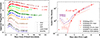 |
Fig. 2. Left: UV and optical light curves of SN 2024igg. The phase is with respect to the B-band maximum (MJD = 60452.10; see Sect. 3.2). The data in different filters are shown with different colors and are shifted vertically for better display. The corresponding instruments are indicated in the legend. Right: Power-law fit to the early-time ZTF r-band light curve of SN 2024igg. The r-band data of SN 2024igg used to fit the power law are shown as red circles. The last non-detections from ZTF r and ATLAS o are plotted as inverted triangles. For comparison, the Clear-band data of SN 2020hvf and the TESS observations of SN 2021zny are shown as dotted and dashed-dotted lines, respectively. The flux densities of SN 2024igg are converted from observed magnitudes and are then scaled to the first detection point. For SNe 2020hvf and 2021zny, the phases are shifted to align their explosion time to the last non-detection of SN 2024igg in ZTF r, and their flux densities are scaled to match at +1.3 (salmon) and +3.5 days (purple). |
To estimate the time of first light, we tried to fit a power law to the ZTF r-band rise phase of the light curve using the data points where the SN flux was ≲40% of its peak value,
 (1)
(1)
where Fr is the flux in the r band, A is the scale factor, t0 is the time of first light, and α is the power-law index. The best fit is shown in the right panel of Figure 2. We found that a simple power law, with t0 = 60435.09 ± 0.16 (MJD) and α = 1.85 ± 0.09, can roughly describe the rise points. This t0 corresponds to a rise time of only about 17 days to B-band maximum, however, which is much shorter than the average rise time of 22.0 ± 3.8 days of 03fg-like SNe (Ashall et al. 2021). This apparent difference may be partly alleviated if the actual explosion preceded t0 owing to a dark phase. Even when we adopted the last non-detection as the explosion epoch, the rise time is still shorter than 18.5 days, possibly shorter than that of any other 03fg-like SN.
An early excess that deviates from a simple power-law rise is expected if the SN ejecta and CSM interact, which has been observed in several 03fg-like SNe such as SN 2020hvf (Jiang et al. 2021) and SN 2021zny (Dimitriadis et al. 2023). No strong early excess is detected in SN 2024igg due to the simple power-law rise, but this might be caused by the brief (∼1 day) excess phase being in observational gaps. Specifically, when we shift the phases of SNe 2020hvf and 2021zny to align their explosion times to the last non-detection of SN 2024igg and scale the flux densities to that around the first detection of SN 2024igg, their early excess would have faded before the first detection of SN 2024igg. Another reason for this non-detection might be the rather shallow and poorly constraining ATLAS o-band limit.
We note that matching the light curves at the first detection of SN 2024igg results in significant differences between the light curves of SN 2024igg and the comparison samples at ∼ + 2 days after t0. To test the robustness of our conclusions, we performed an alternative scaling by matching the flux densities at +3.5 days. Under this alternative scaling, SN 2024igg is fainter than SNe 2020hvf and 2021zny at days +1 to +2. This might be interpreted as evidence of an early excess that is at least weaker than in the comparison SNe. However, an alternative and more straightforward explanation, in our view, is that SN 2024igg has a shorter and steeper rise than SNe 2020hvf and 2021zny, which would naturally produce the observed differences regardless of the scaling method.
In Figure 3 we compare the UV and optical light curves and colors of SN 2024igg with those of several well-observed SNe Ia, including the normal SN 2011fe (Firth et al. 2015; Zhang et al. 2016b; Graham et al. 2017) and five 03fg-like objects: SNe 2009dc (Contreras et al. 2010; Taubenberger et al. 2011; Silverman et al. 2012), 2020esm (Dimitriadis et al. 2022), 2020hvf (Jiang et al. 2021), 2021zny (Dimitriadis et al. 2023), and ASASSN-15hy (Lu et al. 2021). The first two data points of B − V color of SN 2024igg were calculated using UVOT.B and UVOT.V, since they are earlier than the ground-based observations and the response curves are similar. SN 2024igg has a relatively low luminosity in the optical bands among 03fg-like SNe Ia. It is ∼1 mag fainter than SNe 2020esm, 2020hvf, and 2009dc. Initially, SN 2024igg exhibits a lower B-band luminosity than SN 2011fe, although this trend reverses at t ≳ +25 days after B-band maximum because its decline rate (Δm15(B) = 0.90 ± 0.08) is slower than that of SN 2011fe (Δm15(B) = 1.18 ± 0.03; Zhang et al. 2016b). We analyzed the position of SN 2024igg in the B-band WLR in Figure 4 and found it below the Lira-Phillips relation of normal SNe Ia. Despite the relatively low optical luminosity, SN 2024igg shows remarkable similarities to other 03fg-like SNe in terms of (1) high UV luminosity (UVW2 < −18 mag at t ≈ −10 days), (2) low decline rate (Δm15(B) < 1.0 mag), and (3) absence of a prominent i-band secondary maximum that is clearly seen in normal SN 2011fe. These features are also shared by ASASSN-15hy, another less luminous 03fg-like object (MB ≈ −19.14 mag). ASASSN-15hy is much more luminous in the i band and less luminous in the UVW2 band than SN 2024igg, however, suggesting diversity even among the less luminous 03fg-like objects.
 |
Fig. 3. Light-curve and color comparisons of SN 2024igg with a typical normal Type Ia SN 2011fe and five 03fg-like objects: SNe 2009dc, 2020esm, 2020hvf, 2021zny, and ASASSN-15hy. All light curves and colors have been corrected for total reddening. The light curves are shown in absolute magnitude. The I-band light curves of SN 2020hvf and 2011fe have been transformed to AB magnitude (Oke & Gunn 1983). |
 |
Fig. 4. Comparison of the B-band light-curve decline rate and the absolute maximum magnitude for a sample of SNe Ia. SN 2024igg is emphasized as a red triangle. Normal SNe Ia from the Pantheon samples (Scolnic et al. 2018) are shown as gray dots. The solid black curve represents the best-fit Lira-Phillips relation. The 03fg-like sample, shown as blue triangles, is taken from Ashall et al. (2021) except for SNe 2009dc (Taubenberger et al. 2011), 2020esm (Dimitriadis et al. 2022), 2020hvf (Jiang et al. 2021), and 2021zny (Dimitriadis et al. 2023). |
The B − V color of SN 2024igg evolves blueward before the B-band maximum, similar to normal SN 2011fe. For UVM2 − UVW1, however, SN 2024igg and SN 2011fe show inverse evolution trends at t ≳ −10 d: SN 2024igg reddens, while SN 2011fe continues blueward. Consistent with the findings of Hoogendam et al. (2024) for 03fg-like SNe, SN 2024igg is separated from SN 2011fe by UVM2 − UVW1 ≳ 1.0 mag at t ≈ −10 days relative to B-band maximum. Together with the g − r color that continuously reddens from peak up to about +30 days and the decline of the UV flux proportion indicated by UVOT.U − UVOT.B and UVW1 − UVOT.B colors even before the peak luminosity, these characteristics of SN 2024igg again resemble other 03fg-like objects. We note a linear evolution of the r − i color of SN 2024igg before B-band maximum. This evolution trend is similar to that of SN 2021zny, but the color is redder, which might be due to the strong C IIλ6580 absorption of SN 2024igg, which suppresses the r-band flux.
3.3. Spectral analysis
To display the spectroscopic evolution of SN 2024igg, we present the entire spectral series with labels of some important lines in the left panel of Figure 5, together with spectral comparisons with other well-observed SNe in different phases in the right panel. We note that the last two Pennar spectra are strongly affected by an underlying continuum from the host galaxy, due to the dominant contribution of the host-galaxy nucleus combined with the poor seeing. The comparison SNe include a normal Type Ia SN 2011fe (Zhang et al. 2016b; Stahl et al. 2020) and four 03fg-like objects: SNe 2009dc (Silverman et al. 2011; Taubenberger et al. 2011), 2020esm (Tucker et al. 2020; Dimitriadis et al. 2022), 2020hvf (Srivastav et al. 2023), and 2021zny (Dimitriadis et al. 2023).
 |
Fig. 5. Optical spectral evolution of SN 2024igg and comparison with other SNe Ia. All spectra have been corrected for reddening and host-galaxy redshift. Left: Spectral evolution of SN 2024igg from −13.9 to +134.7 days relative to the B-band maximum. Spectra taken with different telescopes are plotted in different colors as indicated in the top legend, and the phase of each spectrum is shown on the right side. Regions of the main telluric absorption are marked by vertical gray bands. The long solid lines indicate Ca II H&K, Fe IIλ4924, S IIλλ5454, 5640, Si IIλ6355, and Ca IIλλλ8498, 8542, 8662 at −8000 km s−1, while C IIλ6580 is indicated at −10 000 km s−1. Right: Spectral comparison of SN 2024igg and SNe 2009dc, 2011fe, 2020esm, 2020hvf, and 2021zny at selected epochs (t ≈ −15, −7, +15, and +100 days). Spectral features are labeled with short lines in panels (a), (b), and (c). In panel (d), the rest wavelengths of [Co III] λ5893, [Ca II] λ7313, and Ca IIλλλ8498, 8542, 8662 are indicated with dashed gray lines, and those of [Fe II] λλ7155, 7453 are indicated with dotted lime green lines. |
3.3.1. First spectrum at −13.9 days
The first spectrum of SN 2024igg, taken at t ≈ −13.9 days relative to the B-band maximum, shows a blue continuum and weak spectral features except for the prominent feature at ∼6300 Å which has a pseudo-equivalent width (pEW) of ∼90 Å. These characteristics resemble the spectrum of SN 2020esm at −12.6 days, in which the ∼6300 Å feature was attributed to C IIλ6580. We ran the radiative-transfer code TARDIS (Kerzendorf & Sim 2014) to confirm this identification based on a toy model, in which blackbody radiation in the photosphere with a velocity of 13 800 km s−1 was assumed, and the outer ejecta, with a total mass of ∼0.06 M⊙, were composed solely of carbon and oxygen in equal masses. An exponential density profile with an e-fold factor of 2000 km s−1 was adopted. Local thermodynamic equilibrium (LTE) and diluted LTE were assumed for ionization and excitation, respectively. An explosion time of texp = −18.4 days, which is close to the time of the last non-detection and consistent with the fitting result in Section 3.4, was used to calculate the expansion time of the ejecta5.
The simulated spectrum obtained with TARDIS is shown in Figure 6, along with a C/O-rich CSM interaction model spectrum at t ≈ −16.6 days from Maeda et al. (2023). The overall flux of the TARDIS spectrum agrees well with the observed spectrum, indicating good estimates of the distance, extinction, and explosion time of SN 2024igg in this work. The strong C IIλ6580 feature is well reproduced by our configurations, but the carbon line strength at ∼4510 Å is significantly overestimated, which complicates the accurate estimation of the carbon mass. This might be due to the inadequacy of the diluted-LTE excitation treatment for C II. Nevertheless, most of the absorption features in the first spectrum of SN 2024igg can be identified as C II. This is consistent with the expectation of the CSM interaction model, in which a thermonuclear explosion occurs within a dense carbon-rich CSM with a mass of 0.1 M⊙. The usual lines seen in normal SNe Ia (e.g., Fe II at ≲5000 Å, S IIλ6355, and W-shaped S II) are still hidden beneath the photosphere in this phase. An exception might be Fe IIλ5169, which might account for the unidentified absorption near 4950 Å. This feature is absent from our TARDIS spectrum, but is reproduced by the CSM-interaction model. The CSM-interaction model includes additional solar metal composition from neon up to iron-peak elements in the envelope, suggesting that this iron might originate from the progenitor system rather than from explosive nucleosynthesis.
 |
Fig. 6. Comparison of the spectrum of SN 2024igg (solid black) at −13.9 days relative to B-band maximum, the synthetic spectrum using TARDIS (dashed blue), and a spectrum taken from the carbon-rich CSM interaction model (solid orange, labeled CSM_M2023) (Maeda et al. 2023). The spectrum of SN 2024igg has been calibrated by the photometry and corrected for reddening and host redshift. The flux density of the spectrum of CSM_M2023, with a CSM mass of 0.1 M⊙, is multiplied by a factor of 0.14 to match the emission peak at ∼6500 Å for visual comparison. The decomposition of the TARDIS spectrum is also shown in the plot, with the positive emission and negative absorption components labeled as different colors. The absorption features of C II and O I are denoted by vertical lines. |
We note that some features are not reproduced by either our toy model or the CSM model spectrum, especially the P-Cygni profile with a clear emission at ∼5800 Å and a broad absorption blended with other lines at ∼5400–5700 Å, neither of which are seen in other 03fg-like SNe. While the emission at ∼5800 Å might be attributed to a blueshifted C IIλ5890 (the spectrum is C II-dominated, and simplifications in our simulations can explain discrepancies with the model), this identification is rendered unlikely by comparison with SN 2020esm, which also exhibits strong C II. We note that this feature resembles the blueshifted He Iλ5876 of SN 2019odp (Schweyer et al. 2025). Other He lines, such as He Iλ6678, are not seen, possibly because they are weak or blended with C II. The origins of the weak absorption at ∼5470 Å and ∼5570 Å are also unclear. By analogy with the possible Fe IIλ5169 absorption, these features might arise from elements other than carbon and oxygen. For instance, the bluer feature can be attributed to Si IIIλ5740 with a blueshifted velocity of about −14 000 km s−1.
3.3.2. Spectral evolution
The second spectrum of SN 2024igg was obtained at t ≈ −6.5 days. In this epoch, weak absorption of the usual elements begins to appear with a velocity of about −8000 km s−1 (measured from the local minimum), such as Fe IIλ4924, W-shaped S II absorption trough, Si IIλ4130 and λ6355, and Ca II H&K (contaminated by C IIλ3921). These weak features at low velocities, alongside the prominent C IIλ6580 absorption, resemble those of other 03fg-like SNe, except for SN 2020hvf. Notably, the C IIλ6580 line of SN 2024igg has some unique properties in this epoch. In other 03fg-like SNe, C IIλ6580 has a strength comparable to or less than Si IIλ6355. In SN 2024igg, however, it remains the strongest absorption feature. Moreover, it is overwhelmingly strong (pEW ≈ 66 Å) compared to any other 03fg-like SNe (pEW ≲ 30 Å; Ashall et al. 2021) in this epoch. Ashall et al. (2021) found a negative correlation between the Si II velocity and the strength of C II among 03fg-like SNe, which also holds for SN 2024igg, as the Si IIλ6355 velocity of −8000 km s−1 is also among the lowest ever recorded for this subtype of SN Ia. The C IIλ6580 absorption is likely detached above the photosphere, as it has a sharp profile and a higher velocity (about −10 000 km s−1) than Si II. The line opacity scales with the density, and this line profile therefore implies that the carbon density peaks around −10 000 km s−1 and drops rapidly toward the inner region.
The left panel of Figure 5 shows that almost all the line velocities evolve slowly before the lines vanish, suggesting that line-forming regions are narrow. An exception is C IIλ6580, which suddenly broadens to a flat profile and drops to ∼ − 7000 km s−1 around peak, possibly due to the existence of another component of carbon in the inner layer. To quantitatively analyze the line velocity evolution, we performed Gaussian fits to Fe IIλ4924 and S IIλ5640. For Si IIλ6355 and C IIλ6580, we fit the features simultaneously using a Gaussian component and an asymmetric Gaussian component with different left and right widths to account for the strongly asymmetric profile of C IIλ6580. At t ≳ +3.9 days, we fit only the Si IIλ6355 absorption because C IIλ6580 becomes weak and noisy. The resulting line velocity evolution from −6.5 to +14.8 days is shown in Figure 7. The slowly evolving velocities of Fe II, S II, and Si II, and the velocity drop of C II around peak, are consistent with the behavior seen in Figure 5.
 |
Fig. 7. Evolution of line velocities in SN 2024igg from −6.5 to +14.8 days relative to the B-band maximum. The different spectral lines are indicated by different colors and symbols. |
As SN 2024igg evolves at t ≈ +14.8 days, Si IIλ6355 weakens, C IIλ6580 and the W-shaped S II disappear, and the Fe II lines become more prominent. While the spectrum of SN 2011fe shows a strong and blended Ca II near-infrared (NIR) triplet, the spectrum of SN 2024igg exhibits a relatively weak but separated Ca IIλ8662 and a blend of Ca IIλλ8498, 8542, bearing a strong resemblance to that of SN 2009dc. By t ≈ +100 days, SN 2024igg enters the early nebular phase when the outer ejecta become moderately transparent. Forbidden lines such as [Fe II], [Fe III], and [Co III] are seen in spectra of 03fg-like and normal SNe Ia in this phase. A key distinction of SN 2024igg from SN 2011fe is the resolved lines, especially at redder wavelengths. This characteristic, combined with its centrally peaked Ca II, is again similar to SNe 2009dc and 2021zny. In contrast, the lines in SN 2020esm appear to be broader, and its Ca II lines are blueshifted.
More resolved lines appear in the spectrum taken at t ≈ +134.7 days, in which we identified forbidden emissions from [Co III] λ5893 (weighted average of the doublet), [Ca II] λ7313 (weighted average of the doublet), and [Fe II] λλ7155, 7453, all peaking at their rest wavelengths. Other 03fg-like SNe also show [Ca II], but they do not reveal the resolved [Co III] and [Fe II] at rest. Although a narrow line is also present near 7155 Å in SN 2021zny, it might not be attributed to [Fe II] λ7155 because the spectrum has a low signal-to-noise ratio and the corresponding [Fe II] λ7453 line (sharing the same upper level) is not visible.
3.4. Pseudo-bolometric light curve
We constructed the pseudo-bolometric (1600–24 000 Å) light curve of SN 2024igg using Swift UVW2, UVM2, UVW1, U, and ground-based BgVri photometry. The UV and optical luminosities were calculated by directly integrating the photometry flux densities. To estimate the NIR luminosity of SN 2024igg, we assumed a similar ratio of the NIR to the optical luminosity to that of SN 2009dc, which shows a similar color evolution in r − i (after peak) and g − r. We caution, however, that SN 2009dc is much more luminous than SN 2024igg, and the NIR flux proportion varies significantly among 03fg-like SNe (Ashall et al. 2021). More details of the calculations can be found in Appendix B.
The pseudo-bolometric light curve of SN 2024igg from −13.3 to +70.7 days is shown in Figure 8, in which we also include those of SNe 2009dc, 2011fe (Zhang et al. 2016b), and 2020esm. The bolometric light curve of SN 2009dc was recalculated using the photometry from several sources (Contreras et al. 2010; Taubenberger et al. 2011; Silverman et al. 2012; Friedman et al. 2015). As expected from the light-curve comparisons in Section 3.2, SN 2024igg has a relatively low bolometric luminosity compared to other 03fg-like objects such as SNe 2009dc and 2020esm, but it is still more luminous than SN 2011fe due to its high UV luminosity. The decline rate of the pseudo-bolometric light curve of SN 2024igg is stable, similar to those of the 03fg-like but different from that of SN 2011fe, which shows a relatively fast decline during the first ∼15 days after peak brightness. We performed a fourth-order polynomial fit to the pseudo-bolometric light curve and obtained a peak time of tpeak, bol = 60450.75 ± 0.39 (MJD), which is earlier than the B-band maximum by ∼1.34 days, and a peak luminosity of Lpeak, bol = (1.31 ± 0.18)×1043 erg s−1.
 |
Fig. 8. Comparison of the bolometric light curves of SN 2024igg (black circles) with those of SNe 2009dc (red diamonds), 2011fe (green stars), and 2020esm (blue triangles). The best-fit model from TRANSFIT for SN 2024igg is overplotted as a blue line, and the corresponding explosion time is indicated by the dashed gray line. |
Assuming that the pseudo-bolometric luminosity of SN 2024igg is only due to the radioactive decay of 56Ni, we used the numerical light-curve fitting tool TRANSFIT (Liu et al. 2025b) to estimate the mass of 56Ni (MNi) synthesized in the explosion and the total ejecta mass (Mej). Compared to the commonly used Arnett analytic model (Arnett 1982), TRANSFIT solves the time-dependent energy balance and photon diffusion numerically, and it thus does not rely on the restrictive assumptions of a single-zone and strictly homologous or instantaneous deposition treatment. This allows a more flexible and self-consistent mapping between Mej, MNi, EK, and the light-curve shape and is well suited for Bayesian inference with robust uncertainty quantification. The best fit is presented in Figure 8, which corresponds to  and
and  (distance error incorporated). More details of the fitting and the Markov chain Monte Carlo (MCMC) corner plot can be found in Appendix B. The fitting also gives an explosion time relative to B-band maximum of
  days, which is ∼1.5 days before the time of first light estimated by the power-law fit in Section 3.2. We note that this difference is not due to the bolometric corrections or another energy source at early times, as an Arnett model yields an explosion time at ∼ − 16.9 days, consistent with that of the power-law fit. We suggest that this difference supports a delay between the explosion and the first light powered by 56Ni. We also note that the prior requiring the explosion occurs after the last ZTF r-band non-detection is a significant constraint on the TRANSFIT fit. Without this prior, the fit would prefer a longer rise time (see the truncated posterior in Fig. B.1), leading to higher Mej and MNi, and a more centrally distributed 56Ni. This prior is physically motivated: the non-detection is deep, and the spectral analysis in Section 3.3 indicates CSM-interaction radiation shortly after explosion. We therefore consider this prior to be reliable and suggest that the explosion time is close to that of the last non-detection.
We note that Mej is strongly correlated with another fitting parameter, the scaled velocity vsc (Arnett 1982). If we had estimated vsc using the Si velocity at peak (∼8000 km s−1) instead of the fitting one (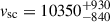 km s−1), as some studies did (e.g., Bora et al. 2024), Mej would drop to only ∼1 M⊙ below MCh. To validate the fitting results, we also used the PYBOLOSN code (Scalzo et al. 2014) to estimate Mej, MNi, and vsc of SN 2024igg. Assuming a rise time to the peak bolometric luminosity of trise, bol = 15.65 ± 1.50 days (limited by the last non-detection and the first detection in ZTF r), we obtained
  ,
,  , and
, and  km s−1, all of which are consistent with the TRANSFIT results within the uncertainties. We note that TRANSFIT and PYBOLOSN infer identical 56Ni masses, even though the explosion time obtained with TRANSFIT is roughly 1.4 days earlier than the estimate based on PYBOLOSN. This might be related to the small differences in the peak time and peak luminosity of the TRANSFIT fit compared to those obtained from the polynomial fit. In addition, the diffusion delay of gamma-ray energy through the ejecta (accounted for in TRANSFIT and PYBOLOSN, but implemented differently) can also affect the estimation of MNi.
4. Discussion
The photometric and spectroscopic observations of SN 2024igg, such as the slowly declining light curve, blue UV−optical colors, and strong carbon features, indicate that this SN is a member of the 03fg-like subclass of SNe Ia. These SNe Ia are thought to explode inside a carbon-rich CSM given their prominent and long-lived C II features (e.g., Lu et al. 2021; Ashall et al. 2021; Dimitriadis et al. 2023), especially for SN 2020esm, whose early-time spectra are dominated by carbon and oxygen absorption (Dimitriadis et al. 2022). The C II-dominated first spectrum of SN 2024igg, with even stronger C II line strengths and absence of Si II compared to SN 2020esm, further supports the carbon-rich CSM interaction model (Maeda et al. 2023). Specifically, the interaction with the CSM leads to the formation of a photosphere within the swept-up carbon-rich envelope. This outer photosphere effectively masks the elemental signatures of the underlying SN ejecta; thus, only features from the CSM itself are detectable at very early times. These features are more prominent in the first spectrum of SN 2024igg possibly due to its observation in an even earlier phase than that of SN 2020esm.
Other observational properties of SN 2024igg also find a unified explanation in the context of CSM interaction. The luminous UV excess, relative to normal SNe Ia, might be interpreted as a reduction in line blanketing because iron-group elements are hidden. Concurrently, the mass gain from the interaction consistently accounts for the marginally super-Chandrasekhar mass and the slowly declining light curve. Furthermore, as the ejecta are decelerated and compressed by the CSM (Noebauer et al. 2016), the spatial extent of line formation is reduced, leading to the observed weak absorption lines with low and slowly evolving velocities (Dessart & Hillier 2005b,a; Dessart et al. 2014). Based on the persistence of line velocities near −10 000 km s−1 for C IIλ6580 and −8000 km s−1 for lines of intermediate-mass elements (IMEs), we speculate that the majority of the SN ejecta were compressed to ≲–10 000 km s−1 and a local density peak formed at about –8000 km s−1.
The carbon-rich CSM of 03fg-like SNe might stem from the classical double-degenerate (DD) scenario (Webbink 1984), in which a thermonuclear explosion is triggered on a secular timescale (much longer than a dynamical timescale) after the onset of a WD-WD merger. The secondary C/O WD is totally disrupted, forming a C/O Keplerian disk (Yoon et al. 2007) that subsequently accretes onto the primary. Although the primary WD might evolve to an ONeMg WD that subsequently collapses to a neutron star in this context (Saio & Nomoto 1985, 1998), this could be avoided in some cases, and a thermonuclear explosion might be eventually triggered if the WD mass reached the MCh limit (Yoon et al. 2007). Different from the slow evolution of the classical scenario, the thermonuclear explosion might also be triggered during the dynamical merger of the WD binary (dubbed as “violent merger”; Pakmor et al. 2012). Although the ejected material during the dynamical merger might be confined owing to the short timescale in this scenario, a wind driven by super-Eddington accretion before the dynamical merger might form an extended CSM (Inoue et al. 2026). We also note that an aspherical explosion of the violent merger is supported by the high intrinsic polarization observed in 03fg-like SNe 2021zny and 2022ilv (Nagao et al. 2024). Although SN 2009dc shows low polarization at early times, the clearly shifted nebular lines in its near-infrared spectra also suggest an aspherical explosion (O’Hora et al. 2025). For SN 2024igg, however, the absence of clear shifts in its nebular-phase forbidden lines disfavors an aspherical explosion.
In the core-degenerate (CD) scenario (Kashi & Soker 2011), a massive WD produced by the merger of a WD with the degenerate core of an AGB star can explode as an SN Ia. In this picture, if the envelope of the AGB star is not completely ejected when the explosion occurs, it would serve as a carbon-rich CSM and interact with the SN ejecta (Hsiao et al. 2020; Lu et al. 2021; Ashall et al. 2021). As the essence of the CD scenario is also a double WD merger, the main observational difference from the classical double-degenerate (DD) scenario probably stems from the AGB star envelope, which might be H-rich and/or He-rich. An emission line possibly associated with blueshifted He Iλ5876 was found in the earliest spectrum of SN 2024igg, but we cannot reproduce it with He using the current treatments in TARDIS; a full non-LTE treatment is required to confirm this identification.
Although we favor a CSM-interaction model that would produce a flux excess at early times, we chose to fit the bolometric light curve of SN 2024igg with an exclusively 56Ni-powered model to estimate its ejecta parameters because the interaction may have ceased before the first bolometric light-curve point at ∼ − 13.3 days as the power-law rise of the r-band light curve indicates no flux excess since ∼−15.5 d. We caution, however, that an exclusively 56Ni-powered model might be not suitable for all 03fg-like objects, particularly those with very luminous and slowly rising light curves such as SN 2009dc, in which the interaction can have lasting effects on the peak. As the luminosity is moderate and the inferred ejecta mass marginally exceeds MCh, SN 2024igg can come from a MCh explosion, such as a delayed-detonation (e.g., Gamezo et al. 2005; Seitenzahl et al. 2013) within a dense carbon-rich CSM with a mass of ∼0.1 M⊙. The [C I] and [O I] lines, which are powerful for constraining the explosion mechanism (e.g., Liu et al. 2025a), are not detected in SN 2024igg, but this might be due to the absence of observations at sufficiently late epochs.
5. Conclusions
We presented and analyzed photometric and spectroscopic observations of SN 2024igg. Although it has a relatively low optical luminosity (Mmax(B) = − 18.99 ± 0.15 mag) and short rise time (shorter than 18.5 days to B-band maximum), it shares many characteristics with other 03fg-like SNe, including the high UV flux, blue UV−optical colors, slowly declining light curve (Δm15(B) = 0.90 ± 0.08 mag), lack of a prominent i-band secondary maximum, strong and long-lived C II, and weak spectral features of IMEs and iron-group elements at early times. On the other hand, this SN exhibits the strongest C IIλ6580 ever detected in an 03fg-like SN, with the pEWs of ∼90 Å and ∼66 Å at t ≈ −13.9 and −6.5 days relative to B-band maximum, respectively. Remarkably, the line velocities of IMEs are already as low as about −8000 km s−1 at t ≈ −6.5 days and evolve slowly until the lines disappear. Together with the C II-dominated spectrum at t ≈ −13.9 days, these properties of SN 2024igg strongly support the idea that this SN exploded within a carbon-rich CSM, which might originate from the debris of the donor WD in a double WD merger or the envelope of an AGB star. As the forbidden lines in the early nebular-phase spectrum are unshifted, we suggest that this SN originates from a symmetric explosion that is triggered on a secular timescale after the merging occurred.
Data availability
Table A.2 is available at the CDS via https://cdsarc.cds.unistra.fr/viz-bin/cat/J/A+A/711/A262. The spectra are available through the Weizmann Interactive Supernova Data Repository (WISeREP) (https://www.wiserep.org/).
Acknowledgments
We thank the anonymous referee for constructive comments which helped improve the manuscript. This work is supported by the National Natural Science Foundation of China (NSFC grants 12288102, 12033003, 11633002) and the Tencent Xplorer Prize. We thank Yi Yang for his contributions to the Keck proposal development and for assisting with the SN 2024igg observations carried out by the U.C. Berkeley group. A.V.F.’s group at U.C. Berkeley received financial assistance from the Christopher R. Redlich Fund, as well as donations from Gary and Cynthia Bengier, Clark and Sharon Winslow, Alan Eustace and Kathy Kwan, Timothy and Melissa Draper, Briggs and Kathleen Wood, Ellyn and Alan Seelenfreund (W.Z. is a Bengier-Winslow-Eustace Specialist in Astronomy, T.G.B. is a Draper-Wood-Seelenfreund Specialist in Astronomy), and numerous other donors. Y.-Z.C. is supported by NSFC grant 12303054, the National Key Research and Development Program of China (grant 2024YFA1611603), and the Yunnan Fundamental Research Projects (grants 202401AU070063, 202501AS070078). A.P., A.R., and G.V. acknowledge support from the PRIN-INAF 2022, “Shedding light on the nature of gap transients: from the observations to the models”. A.R., G.V. and Y.-Z. C. are also supported by the SOXS project (PI S. Campana). J.-J. Z. and Y.-Z. C. are supported by the International Centre of Supernovae, Yunnan Key Laboratory (grant 202302AN360001). J.-J. Zhang is supported by the National Key R&D Program of China (grant 2021YFA1600404), NSFC grant 12173082, the Yunnan Province Foundation (grant 202201AT070069), the Top-notch Young Talents Program of Yunnan Province, and the Light of West China Program provided by the Chinese Academy of Sciences. We thank the staff at the various observatories where data were obtained. A major upgrade of the Kast spectrograph on the Shane 3 m telescope at Lick Observatory, led by Brad Holden, was made possible through generous gifts from the Heising-Simons Foundation, William and Marina Kast, and the University of California Observatories. Research at Lick Observatory is partially supported by a generous gift from Google. Some of the data presented herein were obtained at the W. M. Keck Observatory, which is operated as a scientific partnership among the California Institute of Technology, the University of California, and NASA; the observatory was made possible by the generous financial support of the W. M. Keck Foundation. This work is partially based on observations collected at Copernico and Schmidt telescope (Asiago, Mt. Ekar, Italy) of the INAF – Osservatorio Astronomico di Padova, and at the Galileo telescope (Asiago, Mt. Pennar, Italy) of the Padova University. This work is also based on observations made in the Observatorios de Canarias del IAC with the Telescopio Nazionale Galileo, operated on the island of La Palma by INAF at the Observatorio del Roque de los Muchachos under the program A50TAC_41 (PI G. Valerin). This work was partially supported by the Open Project Program of the Key Laboratory of Optical Astronomy, National Astronomical Observatories, Chinese Academy of Sciences. Funding for the LJT has been provided by the CAS and the People’s Government of Yunnan Province. The LJT is jointly operated and administrated by YNAO and Center for Astronomical Mega-Science, CAS. ZTF is supported by the U.S. NSF under grants AST-1440341 and AST-2034437, and a collaboration including current partners Caltech, IPAC, the Oskar Klein Center at Stockholm University, the University of Maryland, the University of California (Berkeley), the University of Wisconsin at Milwaukee, University of Warwick, Ruhr University, Cornell University, Northwestern University, and Drexel University. Operations are conducted by COO, IPAC, and UW. This research made use of TARDIS, a community-developed software package for spectral synthesis in supernovae (Kerzendorf & Sim 2014; Kerzendorf et al. 2026). The development of TARDIS received support from GitHub, the Google Summer of Code initiative, and from ESA’s Summer of Code in Space program. TARDIS is a fiscally sponsored project of NumFOCUS. TARDIS makes extensive use of Astropy and Pyne. This work makes use of the NASA/IPAC Extragalactic Database, which is funded by NASA and operated by the California Institute of Technology.
References
- Arnett, W. D. 1982, ApJ, 253, 785 [Google Scholar]
- Ashall, C., Lu, J., Hsiao, E. Y., et al. 2021, ApJ, 922, 205 [NASA ADS] [CrossRef] [Google Scholar]
- Becker, A. 2015, Astrophysics Source Code Library [record ascl:1504.004] [Google Scholar]
- Bora, Z., Könyves-Tóth, R., Vinkó, J., et al. 2024, PASP, 136, 094201 [Google Scholar]
- Brennan, S. J., & Fraser, M. 2022, A&A, 667, A62 [NASA ADS] [CrossRef] [EDP Sciences] [Google Scholar]
- Brown, P. J., Holland, S. T., Immler, S., et al. 2009, AJ, 137, 4517 [NASA ADS] [CrossRef] [Google Scholar]
- Brown, P. J., Breeveld, A. A., Holland, S., Kuin, P., & Pritchard, T. 2014, Ap&SS, 354, 89 [Google Scholar]
- Chakradhari, N. K., Sahu, D. K., Srivastav, S., & Anupama, G. C. 2014, MNRAS, 443, 1663 [NASA ADS] [CrossRef] [Google Scholar]
- Contreras, C., Hamuy, M., Phillips, M. M., et al. 2010, AJ, 139, 519 [Google Scholar]
- Dessart, L., & Hillier, D. J. 2005a, A&A, 439, 671 [NASA ADS] [CrossRef] [EDP Sciences] [Google Scholar]
- Dessart, L., & Hillier, D. J. 2005b, A&A, 437, 667 [NASA ADS] [CrossRef] [EDP Sciences] [Google Scholar]
- Dessart, L., Blondin, S., Hillier, D. J., & Khokhlov, A. 2014, MNRAS, 441, 532 [NASA ADS] [CrossRef] [Google Scholar]
- Dimitriadis, G., Foley, R. J., Arendse, N., et al. 2022, ApJ, 927, 78 [NASA ADS] [CrossRef] [Google Scholar]
- Dimitriadis, G., Maguire, K., Karambelkar, V. R., et al. 2023, MNRAS, 521, 1162 [NASA ADS] [CrossRef] [Google Scholar]
- Fan, Y.-F., Bai, J.-M., Zhang, J.-J., et al. 2015, RAA, 15, 918 [Google Scholar]
- Filippenko, A. V. 1982, PASP, 94, 715 [Google Scholar]
- Filippenko, A. V. 1997, ARA&A, 35, 309 [NASA ADS] [CrossRef] [Google Scholar]
- Firth, R. E., Sullivan, M., Gal-Yam, A., et al. 2015, MNRAS, 446, 3895 [NASA ADS] [CrossRef] [Google Scholar]
- Fitzpatrick, E. L. 1999, PASP, 111, 63 [Google Scholar]
- Friedman, A. S., Wood-Vasey, W. M., Marion, G. H., et al. 2015, ApJS, 220, 9 [NASA ADS] [CrossRef] [Google Scholar]
- Gaia Collaboration (Montegriffo, P., et al.) 2023, A&A, 674, A33 [CrossRef] [EDP Sciences] [Google Scholar]
- Gamezo, V. N., Khokhlov, A. M., & Oran, E. S. 2005, ApJ, 623, 337 [NASA ADS] [CrossRef] [Google Scholar]
- Gehrels, N., Chincarini, G., Giommi, P., et al. 2004, ApJ, 611, 1005 [Google Scholar]
- Graham, M. L., Kumar, S., Hosseinzadeh, G., et al. 2017, MNRAS, 472, 3437 [CrossRef] [Google Scholar]
- Guttman, O., Shenhar, B., Sarkar, A., & Waxman, E. 2024, MNRAS, 533, 994 [Google Scholar]
- Hillebrandt, W., & Niemeyer, J. C. 2000, ARA&A, 38, 191 [Google Scholar]
- Hoogendam, W. B., Shappee, B. J., Brown, P. J., et al. 2024, ApJ, 966, 139 [NASA ADS] [CrossRef] [Google Scholar]
- Howell, D. A., Sullivan, M., Nugent, P. E., et al. 2006, Nature, 443, 308 [Google Scholar]
- Hsiao, E. Y., Hoeflich, P., Ashall, C., et al. 2020, ApJ, 900, 140 [NASA ADS] [CrossRef] [Google Scholar]
- Huang, F., Li, J.-Z., Wang, X.-F., et al. 2012, RAA, 12, 1585 [Google Scholar]
- Inoue, Y., Maeda, K., Nagao, T., & Matsumoto, T. 2026, ApJ, 997, 312 [Google Scholar]
- Jiang, J.-A., Maeda, K., Kawabata, M., et al. 2021, ApJ, 923, L8 [NASA ADS] [CrossRef] [Google Scholar]
- Kashi, A., & Soker, N. 2011, MNRAS, 417, 1466 [NASA ADS] [CrossRef] [Google Scholar]
- Kerzendorf, W. E., & Sim, S. A. 2014, MNRAS, 440, 387 [NASA ADS] [CrossRef] [Google Scholar]
- Kerzendorf, W., Sim, S., Vogl, C., et al. 2026, https://doi.org/10.5281/zenodo.18210479 [Google Scholar]
- Khokhlov, A., Mueller, E., & Hoeflich, P. 1993, A&A, 270, 223 [NASA ADS] [CrossRef] [Google Scholar]
- Liu, J., Wang, X., Yang, Y., et al. 2025a, ApJ, 982, L18 [Google Scholar]
- Liu, L.-D., Zhang, Y.-H., Yu, Y.-W., et al. 2025b, ApJ, 992, 20 [Google Scholar]
- Lu, J., Ashall, C., Hsiao, E. Y., et al. 2021, ApJ, 920, 107 [NASA ADS] [CrossRef] [Google Scholar]
- Maeda, K., Jiang, J.-A., Doi, M., Kawabata, M., & Shigeyama, T. 2023, MNRAS, 521, 1897 [NASA ADS] [CrossRef] [Google Scholar]
- Meissner, A., Young, A. R., Martin, A. A., et al. 2024, TNS Classif. Rep., 2024-1433, 1 [Google Scholar]
- Miller, J., & Stone, R. 1993, Lick Obs (Tech. rep., Tech. Rep. 66. Lick Obs., Santa Cruz) [Google Scholar]
- Mould, J. R., Huchra, J. P., Freedman, W. L., et al. 2000, ApJ, 529, 786 [Google Scholar]
- Munoz-Arancibia, A., Mourao, A., Forster, F., et al. 2024, TNSTR, 2024-1413, 1 [Google Scholar]
- Nagao, T., Maeda, K., Mattila, S., et al. 2024, A&A, 687, L19 [NASA ADS] [CrossRef] [EDP Sciences] [Google Scholar]
- Noebauer, U. M., Taubenberger, S., Blinnikov, S., Sorokina, E., & Hillebrandt, W. 2016, MNRAS, 463, 2972 [NASA ADS] [CrossRef] [Google Scholar]
- Nomoto, K., Iwamoto, K., & Kishimoto, N. 1997, Science, 276, 1378 [NASA ADS] [CrossRef] [Google Scholar]
- O’Hora, J., Ashall, C., Shahbandeh, M., et al. 2025, ApJ, 984, 34 [Google Scholar]
- Oke, J. B., & Gunn, J. E. 1983, ApJ, 266, 713 [NASA ADS] [CrossRef] [Google Scholar]
- Oke, J. B., Cohen, J. G., Carr, M., et al. 1995, PASP, 107, 375 [Google Scholar]
- Pakmor, R., Kromer, M., Taubenberger, S., et al. 2012, ApJ, 747, L10 [NASA ADS] [CrossRef] [Google Scholar]
- Perley, D. A. 2019, PASP, 131, 084503 [Google Scholar]
- Perlmutter, S., Aldering, G., Goldhaber, G., et al. 1999, ApJ, 517, 565 [Google Scholar]
- Phillips, M. M. 1993, ApJ, 413, L105 [Google Scholar]
- Phillips, M. M., Lira, P., Suntzeff, N. B., et al. 1999, AJ, 118, 1766 [Google Scholar]
- Riess, A. G., Filippenko, A. V., Challis, P., et al. 1998, AJ, 116, 1009 [Google Scholar]
- Riess, A. G., Yuan, W., Macri, L. M., et al. 2022, ApJ, 934, L7 [NASA ADS] [CrossRef] [Google Scholar]
- Roming, P. W. A., Kennedy, T. E., Mason, K. O., et al. 2005, Space Sci. Rev., 120, 95 [Google Scholar]
- Saio, H., & Nomoto, K. 1985, A&A, 150, L21 [NASA ADS] [Google Scholar]
- Saio, H., & Nomoto, K. 1998, ApJ, 500, 388 [Google Scholar]
- Scalzo, R., Aldering, G., Antilogus, P., et al. 2014, MNRAS, 440, 1498 [NASA ADS] [CrossRef] [Google Scholar]
- Schlafly, E. F., & Finkbeiner, D. P. 2011, ApJ, 737, 103 [Google Scholar]
- Schweyer, T., Sollerman, J., Jerkstrand, A., et al. 2025, A&A, 693, A13 [NASA ADS] [CrossRef] [EDP Sciences] [Google Scholar]
- Scolnic, D. M., Jones, D. O., Rest, A., et al. 2018, ApJ, 859, 101 [NASA ADS] [CrossRef] [Google Scholar]
- Seitenzahl, I. R., Ciaraldi-Schoolmann, F., Röpke, F. K., et al. 2013, MNRAS, 429, 1156 [NASA ADS] [CrossRef] [Google Scholar]
- Siebert, M. R., Kwok, L. A., Johansson, J., et al. 2024, ApJ, 960, 88 [NASA ADS] [CrossRef] [Google Scholar]
- Silverman, J. M., Ganeshalingam, M., Li, W., et al. 2011, MNRAS, 410, 585 [NASA ADS] [CrossRef] [Google Scholar]
- Silverman, J. M., Foley, R. J., Filippenko, A. V., et al. 2012, MNRAS, 425, 1789 [Google Scholar]
- Srivastav, S., Smartt, S. J., Huber, M. E., et al. 2023, ApJ, 943, L20 [NASA ADS] [CrossRef] [Google Scholar]
- Srivastav, S., Fulton, M., Smith, K. W., et al. 2024, TNSAN, 132, 1 [Google Scholar]
- Stahl, B. E., Zheng, W., de Jaeger, T., et al. 2020, MNRAS, 492, 4325 [NASA ADS] [CrossRef] [Google Scholar]
- Steele, I. A., Smith, R. J., Rees, P. C., et al. 2004, SPIE Conf. Ser., 5489, 679 [Google Scholar]
- Taubenberger, S. 2017, in Handbook of Supernovae, eds. A. W. Alsabti, & P. Murdin (Springer), 317 [Google Scholar]
- Taubenberger, S., Benetti, S., Childress, M., et al. 2011, MNRAS, 412, 2735 [NASA ADS] [CrossRef] [Google Scholar]
- Taubenberger, S., Kromer, M., Hachinger, S., et al. 2013, MNRAS, 432, 3117 [NASA ADS] [CrossRef] [Google Scholar]
- Theureau, G., Hanski, M. O., Coudreau, N., Hallet, N., & Martin, J. M. 2007, A&A, 465, 71 [NASA ADS] [CrossRef] [EDP Sciences] [Google Scholar]
- Tucker, M. A., Payne, A. V., Hinkle, J., et al. 2020, TNS Classif. Rep., 2020-861, 1 [Google Scholar]
- Wang, X., Li, W., Filippenko, A. V., et al. 2008, ApJ, 675, 626 [NASA ADS] [CrossRef] [Google Scholar]
- Webbink, R. F. 1984, ApJ, 277, 355 [NASA ADS] [CrossRef] [Google Scholar]
- Yoon, S. C., Podsiadlowski, P., & Rosswog, S. 2007, MNRAS, 380, 933 [Google Scholar]
- Zhang, J.-C., Fan, Z., Yan, J.-Z., et al. 2016a, PASP, 128, 105004 [Google Scholar]
- Zhang, K., Wang, X., Zhang, J., et al. 2016b, ApJ, 820, 67 [NASA ADS] [CrossRef] [Google Scholar]
IRAF is distributed by the National Optical Astronomy Observatories, which are operated by the Association of Universities for Research in Astronomy, Inc., under cooperative agreement with the U.S. National Science Foundation (NSF).
More details of our TARDIS setup and Python codes are available in GITHUB https://github.com/jl-liu2022/TARDIS_SN2024igg
Appendix A: Photometric and spectroscopic observations
The journal of spectroscopic observations is presented in Table A.1. The photometric data are listed in Table A.2.
Log of optical spectra of SN 2024igg.
Photometric observations of SN 2024igg.
Appendix B: Construction and fitting of the pseudo-bolometric light curve
The pseudo-bolometric light curve of SN 2024igg was constructed using Swift UVW2, UVM2, UVW1, U, and ground-based BgVri photometry. Swift UVOT.B and UVOT.V were used at t ≈ −13.31 and −11.48 days relative to B-band maximum, when the ground-based BV photometry was not yet available. We assumed a linear evolution of the r − i color, as found in Section 3, to estimate the i-band magnitude based on ZTF r. We assumed constant UVW2 − B, UVM2 − B, UVW1 − B, and UVOT.U − B colors at t > +35 days when UV photometry is not available, and note that the UV contribution to the total luminosity is small at this phase. The data were interpolated in each filter at the observed epochs of UVM2 (t < +35 days) and B (t > +35 days) so that the pseudo-bolometric luminosity can be calculated at the same phase. After correcting for the Galactic reddening, the photometric magnitudes were converted to monochromatic fluxes. The spectral energy distribution (SED) was then interpolated linearly and integrated with respect to wavelength, assuming zero flux at the blue edge of the UVW2 band (1600 Å).
To estimate the flux of the 7500–24,000 Å range, beyond the i-band, we assumed that the flux ratio of this range to the optical one (4400–7500 Å) was similar to that of SN 2009dc, which showed a similar color evolution in r − i (after peak) and g − r. Finally, a pseudo-bolometric (1600–24,000 Å) light curve of SN 2024igg from −13.31 to +70.72 days was obtained by combining the UV, optical, and NIR luminosities. The pseudo-bolometric light curve is presented in Table B.1.
Estimated pseudo-bolometric light curve of SN 2024igg.
The TRANSFIT code (Liu et al. 2025b) was used to estimate the mass of 56Ni synthesized in the explosion and the total ejecta mass, assuming that the pseudo-bolometric luminosity of SN 2024igg is only due to the radioactive decay of 56Ni. TRANSFIT is a novel framework that numerically solves a generalized energy-conservation equation, explicitly incorporating time-dependent radiative diffusion, continuous radioactive or central-engine heating, and ejecta expansion dynamics. The 56Ni-powered model includes six parameters: ejecta mass Mej, kinetic energy EK or scaled velocity vsc (EK = 0.5Mejvsc2), 56Ni mass MNi, maximum 56Ni distribution radius xheat (dimensionless within 0–1, in mass space), gray opacity κ, and opacity for gamma-ray photons κγ. Constant opacities κ = 0.1 cm2 g −1 (Dimitriadis et al. 2023) and κγ = 0.025 cm2 (Guttman et al. 2024) were adopted in the fitting. The explosion time texp relative to B-band maximum was included as an additional parameter, which is limited by the last non-detection and the first detection in ZTF r. The MCMC corner plot is shown in Figure B.1, which corresponds to 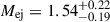 M⊙,
M⊙,  M⊙ (distance error incorporated),
  ,
,  days, and
  km s−1.
 |
Fig. B.1. Corner plot showing the posterior probability distributions for the physical parameters of SN 2024igg obtained with our MCMC analysis using TRANSFIT. The diagonal panels display the marginalized one-dimensional distributions for each, with vertical dashed lines and red solid lines indicating the central 68% credible interval (1σ) and the median. Note that the uncertainty of MNi shown in the plot reflects only the fitting errors. When the distance uncertainty is incorporated, the final result yields |

All Tables
All Figures
|
Fig. 1. TNT 12′×12′ color-composite (B/V/r) image of SN 2024igg and its host galaxy. The reference stars used to calibrate the photometry are marked with circles. The inset shows the zoomed-in region of the SN (indicated with magenta lines) and its host taken on 2024 June 16. |
| In the text | |
|
Fig. 2. Left: UV and optical light curves of SN 2024igg. The phase is with respect to the B-band maximum (MJD = 60452.10; see Sect. 3.2). The data in different filters are shown with different colors and are shifted vertically for better display. The corresponding instruments are indicated in the legend. Right: Power-law fit to the early-time ZTF r-band light curve of SN 2024igg. The r-band data of SN 2024igg used to fit the power law are shown as red circles. The last non-detections from ZTF r and ATLAS o are plotted as inverted triangles. For comparison, the Clear-band data of SN 2020hvf and the TESS observations of SN 2021zny are shown as dotted and dashed-dotted lines, respectively. The flux densities of SN 2024igg are converted from observed magnitudes and are then scaled to the first detection point. For SNe 2020hvf and 2021zny, the phases are shifted to align their explosion time to the last non-detection of SN 2024igg in ZTF r, and their flux densities are scaled to match at +1.3 (salmon) and +3.5 days (purple). |
| In the text | |
|
Fig. 3. Light-curve and color comparisons of SN 2024igg with a typical normal Type Ia SN 2011fe and five 03fg-like objects: SNe 2009dc, 2020esm, 2020hvf, 2021zny, and ASASSN-15hy. All light curves and colors have been corrected for total reddening. The light curves are shown in absolute magnitude. The I-band light curves of SN 2020hvf and 2011fe have been transformed to AB magnitude (Oke & Gunn 1983). |
| In the text | |
|
Fig. 4. Comparison of the B-band light-curve decline rate and the absolute maximum magnitude for a sample of SNe Ia. SN 2024igg is emphasized as a red triangle. Normal SNe Ia from the Pantheon samples (Scolnic et al. 2018) are shown as gray dots. The solid black curve represents the best-fit Lira-Phillips relation. The 03fg-like sample, shown as blue triangles, is taken from Ashall et al. (2021) except for SNe 2009dc (Taubenberger et al. 2011), 2020esm (Dimitriadis et al. 2022), 2020hvf (Jiang et al. 2021), and 2021zny (Dimitriadis et al. 2023). |
| In the text | |
|
Fig. 5. Optical spectral evolution of SN 2024igg and comparison with other SNe Ia. All spectra have been corrected for reddening and host-galaxy redshift. Left: Spectral evolution of SN 2024igg from −13.9 to +134.7 days relative to the B-band maximum. Spectra taken with different telescopes are plotted in different colors as indicated in the top legend, and the phase of each spectrum is shown on the right side. Regions of the main telluric absorption are marked by vertical gray bands. The long solid lines indicate Ca II H&K, Fe IIλ4924, S IIλλ5454, 5640, Si IIλ6355, and Ca IIλλλ8498, 8542, 8662 at −8000 km s−1, while C IIλ6580 is indicated at −10 000 km s−1. Right: Spectral comparison of SN 2024igg and SNe 2009dc, 2011fe, 2020esm, 2020hvf, and 2021zny at selected epochs (t ≈ −15, −7, +15, and +100 days). Spectral features are labeled with short lines in panels (a), (b), and (c). In panel (d), the rest wavelengths of [Co III] λ5893, [Ca II] λ7313, and Ca IIλλλ8498, 8542, 8662 are indicated with dashed gray lines, and those of [Fe II] λλ7155, 7453 are indicated with dotted lime green lines. |
| In the text | |
|
Fig. 6. Comparison of the spectrum of SN 2024igg (solid black) at −13.9 days relative to B-band maximum, the synthetic spectrum using TARDIS (dashed blue), and a spectrum taken from the carbon-rich CSM interaction model (solid orange, labeled CSM_M2023) (Maeda et al. 2023). The spectrum of SN 2024igg has been calibrated by the photometry and corrected for reddening and host redshift. The flux density of the spectrum of CSM_M2023, with a CSM mass of 0.1 M⊙, is multiplied by a factor of 0.14 to match the emission peak at ∼6500 Å for visual comparison. The decomposition of the TARDIS spectrum is also shown in the plot, with the positive emission and negative absorption components labeled as different colors. The absorption features of C II and O I are denoted by vertical lines. |
| In the text | |
|
Fig. 7. Evolution of line velocities in SN 2024igg from −6.5 to +14.8 days relative to the B-band maximum. The different spectral lines are indicated by different colors and symbols. |
| In the text | |
|
Fig. 8. Comparison of the bolometric light curves of SN 2024igg (black circles) with those of SNe 2009dc (red diamonds), 2011fe (green stars), and 2020esm (blue triangles). The best-fit model from TRANSFIT for SN 2024igg is overplotted as a blue line, and the corresponding explosion time is indicated by the dashed gray line. |
| In the text | |
|
Fig. B.1. Corner plot showing the posterior probability distributions for the physical parameters of SN 2024igg obtained with our MCMC analysis using TRANSFIT. The diagonal panels display the marginalized one-dimensional distributions for each, with vertical dashed lines and red solid lines indicating the central 68% credible interval (1σ) and the median. Note that the uncertainty of MNi shown in the plot reflects only the fitting errors. When the distance uncertainty is incorporated, the final result yields |
| In the text | |
Current usage metrics show cumulative count of Article Views (full-text article views including HTML views, PDF and ePub downloads, according to the available data) and Abstracts Views on Vision4Press platform.
Data correspond to usage on the plateform after 2015. The current usage metrics is available 48-96 hours after online publication and is updated daily on week days.
Initial download of the metrics may take a while.