| Issue |
A&A
Volume 709, May 2026
|
|
|---|---|---|
| Article Number | A209 | |
| Number of page(s) | 12 | |
| Section | Extragalactic astronomy | |
| DOI | https://doi.org/10.1051/0004-6361/202659126 | |
| Published online | 19 May 2026 | |
Rate of repeating tidal disruption events with a 5–19 years interval
1
Department of Physics, Anhui Normal University, Wuhu, Anhui, 241002, China
2
South-Western Institute for Astronomy Research, Yunnan University, Kunming, 650500, Yunnan, China
3
CAS Key Laboratory for Researches in Galaxies and Cosmology, Department of Astronomy, University of Science and Technology of China, Hefei, Anhui, 230026, China
4
School of Astronomy and Space Sciences, University of Science and Technology of China, Hefei, Anhui, 230026, China
★ Corresponding author: This email address is being protected from spambots. You need JavaScript enabled to view it.
Received:
26
January
2026
Accepted:
25
March
2026
Abstract
Context. Statistics on tidal disruption events (TDEs) may be contaminated by repeating TDEs (rTDEs), which have been widely discovered in recent years. However, no statistical study has yet examined rTDEs with time intervals longer than 5 years. In addition, the origin of rTDEs remains unclear.
Aims. We aim to search for rTDEs with time intervals longer than 5 years in a well-defined TDE sample and to estimate the rTDE rate and fraction in the sample.
Methods. We used a sample of 16 TDEs at z < 0.05 from the Zwicky Transient Facility (ZTF) Bright Transient Survey (BTS) to search for flares 5–19 years before the ZTF TDEs using the Catalina Real-time Sky Survey (CRTS) light curves. We analyzed archival multi-band data to distinguish between TDEs and supernovae (SNe) and estimated the expected number of SNe that CRTS could detect in the sample.
Results. We identify two rTDE candidates, AT 2019azh and AT 2024pvu, with time intervals of 13.2 and 17.1 years, respectively. The peak luminosities of the CRTS flares are close to those of ZTF flares. For the CRTS flare of AT 2024pvu, we used UV observations from the Galaxy Evolution Explorer (GALEX) near the peak to measure a blackbody temperature of ∼19 500 K, consistent with TDEs and higher than that of SNe. Moreover, we estimate the expected number of SNe in the sample to be ≲0.08, and hence the probability that both CRTS flares are SNe is only 0.3%. Therefore, we rule out the possibility that both CRTS flares are SNe and conclude that both are likely TDEs. Using the two rTDEs, we infer that the TDE rate is two to three orders of magnitude higher than the average over 5–19 years prior to TDE detection. Two rTDEs with intervals of ∼2 years in the sample, together with possible rTDEs missed by CRTS, suggest that rTDEs with intervals of < 20 years may account for 25%–60% of the TDE sample. We interpret rTDEs as repeating partial TDEs. If so, the high fraction of rTDEs suggests that the observed optical TDE rate is overestimated. However, the possibility of independent TDEs cannot be ruled out and requires future observational tests.
Key words: galaxies: nuclei
© The Authors 2026
 Open Access article, published by EDP Sciences, under the terms of the Creative Commons Attribution License (https://creativecommons.org/licenses/by/4.0), which permits unrestricted use, distribution, and reproduction in any medium, provided the original work is properly cited.
This article is published in open access under the Subscribe to Open model. This email address is being protected from spambots. You need JavaScript enabled to view it. to support open access publication.
1. Introduction
A tidal disruption event (TDE) occurs when a star approaches the tidal radius (Rt) of a supermassive black hole (SMBH) and is tidally disrupted (e.g. Hills 1975; Rees 1988):
 (1)
(1)
where R★ and M★ are the radius and mass of the star and MBH is the mass of the SMBH. A TDE can be observed if it occurs outside the event horizon, which sets an upper limit for MBH of ∼3 × 10⁸ M⊙ for Schwarzschild SMBHs and Sun-like stars. Below this limit, TDEs produce a bright UV-optical and/or X-ray flare (Komossa 2015; van Velzen et al. 2020; Saxton et al. 2020) with a light curve roughly following L ∝ t−5/3 in theory (Rees 1988). Its optical spectrum is characterised by a blue continuum with a high and nearly constant blackbody temperature (e.g. Arcavi et al. 2014; Gezari 2021; Yao et al. 2023), different from other impostors, such as supernovae (SNe) or active galactic nucleus (AGN) flares (Zabludoff et al. 2021).
A TDE provides a unique opportunity to discover and statistically analyse inactive SMBHs (e.g. Stone & Metzger 2016; van Velzen 2018), especially at the low-mass end where the classical dynamical method encounters difficulties (Mockler et al. 2026). Thanks to large-area, high-cadence optical surveys such as the All Sky Automated Survey for Supernovae (ASAS-SN; Shappee et al. 2014; Kochanek et al. 2017), the Asteroid Terrestrial impact Last Alert System (ATLAS; Tonry et al. 2018; Smith et al. 2020; Shingles et al. 2021) and the Zwicky Transient Facility (ZTF; Bellm et al. 2019; Masci et al. 2019), as well as X-ray surveys such as extended ROentgen Survey with an Imaging Telescope Array (eROSITA; Predehl et al. 2021), the number of discovered TDEs has increased rapidly in recent years to ≳102 (e.g. van Velzen et al. 2021; Hammerstein et al. 2023; Sazonov et al. 2021; Zhang et al. 2026). Recent rate estimates for optical and X-ray TDEs are  and
and  Mpc−3 yr−1, respectively, or ∼ 2 − 3 × 10⁻⁵ galaxy−1 yr−1 (e.g. Yao et al. 2023; Grotova et al. 2025). The total TDE rate, after accounting for dust-obscured TDEs revealed in the mid-infrared (MIR) bands (∼ 2 × 10⁻⁵ galaxy−1 yr−1, Jiang et al. 2021; Masterson et al. 2024; Yao et al. 2025b), roughly matches the prediction of 10−5 − 10−4 galaxy−1 yr−1 (e.g. Wang & Merritt 2004; Stone et al. 2020) from loss cone theory (e.g. Frank & Rees 1976; Merritt 2013).
The above rate statistics represent average values across all galaxies. However, the TDE rate among galaxies of different types and properties varies greatly (e.g. Chang et al. 2025; Hannah et al. 2025). Observationally, TDEs are preferably hosted in post-starburst galaxies, with a rate enhanced by a factor of a few to several tens (e.g. Liu & Chen 2013; Arcavi et al. 2014; French et al. 2016; Law-Smith et al. 2017; Yao et al. 2023). The origin of the preference remains unclear (see details in Stone et al. 2020).
Another possible issue with TDE rate statistics arises from repeating TDEs (rTDEs), which have been widely observed in recent years. The first candidate was identified in the Seyfert galaxy IC 3599, with one flare detected in X-ray in 1990 (Brandt et al. 1995; Grupe et al. 1995) and another flare detected in both the optical and the X-ray bands in 2009 (Campana et al. 2015; Grupe et al. 2015), although its TDE nature remains under debate (Saxton et al. 2015). The first periodic rTDE is ASASSN-14ko, which has exhibited more than 30 flares to date with a period of 114 days (Payne et al. 2021, 2022, 2023; Huang et al. 2025). Other rTDEs or candidates include AT 2018fyk (Wevers et al. 2023), AT 2020vdq (Somalwar et al. 2025), AT 2022dbl (Lin et al. 2024; Hinkle et al. 2024), eRASSt J045650.3–203750 (Liu et al. 2023, 2024), IRAS F01004-2237 (Sun et al. 2024), AT 2021aeuk (Bao et al. 2024; Sun et al. 2025), AT 2022sxl (Ji et al. 2025), and AT 2023uqm (Wang et al. 2025).
The origin of rTDE remains unclear. A widely accepted model, the repeating partial TDE (rpTDE; Payne et al. 2021), assumes that a single star in an elliptical orbit around an SMBH repeatedly undergoes partial disruption. The most substantial evidence comes from the good periodicity of flares in ASASSN-14ko and AT 2023uqm, with a period of 527 days. The semi-major axis, a, of the star derived from the period is approximately two orders of magnitude larger than Rt, requiring a highly eccentric orbit. Stars on such orbits can be produced through the Hills mechanism (e.g. Hills 1988), although its details remain unclear. To explain the generation of multiple flares, the model requires that the star be partially disrupted while its core survives (e.g. Ryu et al. 2020a,b). This in turn demands that the star’s penetration factor (β = Rt/Rp, where Rp is the periapsis distance) be < 1, unlike the classic fully disrupted events for which β ≥ 1. Besides the rpTDE model, there are other possibilities, such as independent TDEs (Sun et al. 2024), double TDEs (Mandel & Levin 2015), and models involving SMBH binary (SMBHB; Coughlin et al. 2018).
Statistical analysis of rTDEs is essential for studying the TDE rate. On the one hand, if different TDEs observed in one galaxy are independent, the TDE rate therein will be extremely high (∼10−2 − 10−1 galaxy−1 yr−1). This would confirm predictions from some theories, for example, that a close SMBH companion can boost the TDE rate by several orders of magnitude (Ivanov et al. 2005). On the other hand, if multiple TDE flares are physically related, the TDE rate is overestimated because these flares should be regarded as a single event in statistics. If rTDEs account for a significant fraction of current TDE samples, they will substantially contaminate research on the TDE rate and preferences.
Somalwar et al. (2025) explored the fraction of rTDE for the first time using a complete ZTF sample from Yao et al. (2023), containing 33 TDEs. They identified one rTDE using ZTF data and infer a fraction of 1/33, with a 3σ upper limit of ≲40%. However, this fraction may be underestimated, as they did not account for rTDEs with periods longer than 5 years.
The rTDEs with longer time intervals can be studied using historical data such as the Catalina Real-time Sky Survey (CRTS; Drake et al. 2009), which began in 2005 and allows the study of rTDEs with intervals up to ∼20 years. Using CRTS data, Hinkle et al. (2021) and Langis et al. (2026) note two rTDE candidates with time intervals longer than 10 years, AT 2019azh and AT 2024pvu. However, no statistical analyses have studied long-interval rTDEs to date. Furthermore, it is unclear whether these two events are rTDEs, and the possibility of a combination of TDE and SN, as in AT 2021mhg (TDE+SN Ia; Somalwar et al. 2025), cannot be ruled out.
In this work, we conducted a systematic search for rTDE candidates using CRTS data for a well-defined TDE sample, verified their nature, and estimated the fraction and rate of rTDEs. The paper is organised as follows. In section 2, we describe how we selected the rTDE candidates and probed the nature of the CRTS flare of AT 2024pvu using multi-band data. In section 3, we discuss the possibility of SN contamination, estimate the fraction and rate of rTDE, and explore the possible origin. We summarise the results in Section 4. Throughout this paper, we adopted the cosmological constants of H0 = 70 km s−1 Mpc−1, ΩM = 0.3, ΩΛ = 0.7, and Tcmb = 2.725 K, and calculated the luminosity distance using cosmology in Astropy (Astropy Collaboration 2022) based on redshift.
2. Sample selection and data analysis
2.1. Selection of rTDE candidates
We started from the TDE catalogue1 of the ZTF Bright Transient Survey (BTS; Fremling et al. 2020; Perley et al. 2020; Rehemtulla et al. 2024). We adopted a redshift cut of z < 0.05 to increase the detection completeness of TDE flares in the shallower CRTS, and selected 18 ZTF TDEs. One TDE in the sample, AT 2022wtn, is hosted by a galaxy merger, with a centre position in the CRTS catalogue of 7″ away from the TDE position. In this case, any potential flare at the TDE position would be unlikely to be detected in the CRTS light curve, so we removed AT 2022wtn from the sample. We also removed AT 2024tvd, which is reported to be off-nuclear (Yao et al. 2025a). The final sample contains 16 TDEs; Table 1 lists their properties. We also list the time differences between the CRTS observations and the ZTF TDE peak time, as well as the depth of CRTS (expressed as the V-band absolute magnitude MV,limit for 5σ detection). Using CRTS data, we can detect rTDEs with time intervals of 5 − 19 years with depths (MV,limit) ranging from −16.7 to −18.9 in the sample.
Summary of 16 ZTF BTS TDEs at z < 0.05.
We obtained the CRTS single-exposure photometry of their host galaxies from the CRTS Data Release 22, which includes data taken between 2005 and 2013. The CRTS typically obtained sequences of four consecutive exposures per source in a single night. The photometry from these exposures should show no significant differences; we therefore binned the exposures into a single data point. Before binning, we checked for abnormal photometric data by examining whether magnitudes were consistent within the error margin. We required that the standard deviation of the magnitudes be less than three times the root-mean-square of the magnitude errors; otherwise, we discarded all photometry for that night. We adopted the weighted average of the magnitudes as the final magnitude of this night, with weights equal to the reciprocal of the squared magnitude error. The final magnitude error was calculated using the rule of error propagation.
The CRTS took images without a filter and calibrated the photometric data to a pseudo-V magnitude (VCSS) close to the Bessel V magnitude. The difference is related to colour and is expressed as (Drake et al. 2013)
 (2)
(2)
In this work, we studied TDEs with blue B − V colours between −0.2 and 0, resulting in magnitude differences of 0.04–0.052. Thus, we converted all VCSS measurements to V magnitudes by adding 0.046.
To identify flares in the nightly-binned CRTS light curves, we calculated the median of all fluxes as the background value. We then selected > 5σ significant flux excess by requiring that the excess flux over the background exceeds five times the error. We identified a flare when there were at least two consecutive data points with such > 5σ flux excess. Based on this criterion, we detected two flares in the host galaxies of AT 2019azh and AT 2024pvu, which occurred in 2005 and 2006, respectively (Figure 1). We refer to the CRTS flares as AT 2019azh.I and AT 2024pvu.I and the corresponding ZTF flares as AT 2019azh.II and AT 2024pvu.II. Hinkle et al. (2021) and Langis et al. (2026) previously noted these two long-interval rTDE candidates, but they do not provide substantial evidence that the CRTS flares are TDEs.
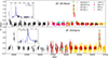 |
Fig. 1. Host-subtracted optical light curves of AT 2019azh and AT 2024pvu. Insert panels show zoomed views of the CRTS flares and the Gaussian+Power-law (GP) models that fit the data. For AT 2024pvu, the observation time of GALEX is indicated by a dashed green line. |
2.2. Light curve analysis
AT 2024pvu.I exhibits a light curve with a fast rise and a slow decline, consistent with those of TDEs, whereas observations detected only the declining phase of AT 2019azh.I. We fit the light curves using a model assuming a Gaussian rise and a power-law decline (hereafter GP model), expressed as:
 (3)
(3)
where tpeak and Lmax are the peak time and peak luminosity of the flare, σrise and t0 imply the timescales of rise and decline, and p is the power-law index of the decline. We performed the fit with the Markov chain Monte Carlo (MCMC) code emcee (Foreman-Mackey et al. 2013). We initially attempted to set p as a free parameter, but the data were too sparse to constrain it. Therefore, we adopted two reasonable p values, p = −5/3 and p = −9/4 for full TDEs (Rees 1988) and partial TDEs (Coughlin & Nixon 2019; Miles et al. 2020), respectively, to constrain the other parameters. The model fits the data well, as shown in the inset panels of Figure 1. Table 2 lists the inferred model parameters. We list the t1/2, decline assuming two different p values, whereas the choice of p hardly influences other parameters. The peak V-band luminosity and rise and decline timescales are all within the range of ZTF TDEs from Yao et al. (2023, hereafter Yao23).
Light-curve model parameters for the two rTDEs.
We also investigated the light curve parameters of the corresponding ZTF flares for comparison. We adopted the parameters for AT 2019azh.II from Yao23 and obtained the parameters for AT 2024pvu.II by fitting the ZTF, ATLAS, and Swift Ultraviolet/Optical Telescope (UVOT; Roming et al. 2005) data (see details in the Appendix A.2) using the model of van Velzen et al. (2021). The model assumes a bolometric light curve given by Eq. (3), and a blackbody spectrum in which TBB varies linearly with time. Table 2 also lists the parameters. For both rTDE candidates, the peak luminosities of the two flares agree within the margin of error. The timescales are also comparable, except that AT 2019azh.II has a longer decline timescale than AT 2019azh.I. The rest-frame time intervals are 13.2 and 17.1 years for AT 2019azh and AT 2024pvu, respectively.
To examine whether any additional flares occurred in these two galaxies between the CRTS and ZTF detections, we collated light-curve data from other surveys, including ASAS-SN, Gaia, and ATLAS. Figure 1 shows all light curves, which reveal no additional significant flares.
2.3. Multi-band analysis of AT 2024pvu.I
Observations of AT 2024pvu.II classify it as a TDE based on its persistent blue colour, the strong and broad He II emission line in the spectrum, and the lack of AGN-like host signatures (Stein et al. 2024). Langis et al. (2026) first reported AT 2024pvu.I using CRTS data, but the literature lacks evidence to exclude the SN possibility and to confirm its TDE nature.
Luminous UV emission and high blackbody temperature are essential features that distinguish TDEs from SNe (e.g. van Velzen et al. 2020; Gezari 2021). Observations by the Galaxy Evolution Explorer (GALEX; (Martin et al. 2005)) captured the host galaxy of AT 2024pvu during the CRTS flare. The observation at MJD = 54010.5 occurred near the peak of the CRTS flare. In both far UV (FUV) and near UV (NUV) images, we detect a point source at the galaxy centre with no extended feature, suggesting that the UV emission is more likely associated with the flare rather than the host galaxy.
To verify whether the host galaxy is responsible for the UV emission, we triggered a new Swift target of opportunity observation (ID:00016768015) in November 2025 (MJD = 60974), after AT 2024pvu.II faded. Figure 2(a) shows that the NUV fluxes are several tens of times lower than those observed by GALEX. To assess any late-time UV emission from AT 2024pvu.II and to measure the host galaxy’s UV contribution more accurately, we collected archival multi-band photometric data from the Sloan Digital Sky Survey (SDSS; York et al. 2000), the Two Micron All Sky Survey (2MASS; Skrutskie et al. 2006), and the Wide-field Infrared Survey Explorer (WISE; Wright et al. 2010). All data were obtained at epochs without flares (see Appendix A.2 for details). We fit the spectral energy distribution (SED) using the Code Investigating GALaxy Emission (CIGALE; Boquien et al. 2019). In the fitting, we assumed that the star formation history can be described by the sum of two exponential decays and adopted the single stellar population templates of Bruzual & Charlot (2003). We accounted for dust attenuation and emission using models from Calzetti et al. (2000) and Dale et al. (2014), and did not include any AGN component. The resultant SED models of the host galaxy, if extrapolated to the UV bands, are consistent with the Swift UV observations in November 2025. However, the synthetic fluxes in the FUV and NUV bands are about two orders of magnitude lower than the observed values from GALEX, indicating that the transient source dominates the UV emission at MJD = 54010.5.
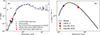 |
Fig. 2. (a): Spectral energy distribution (SED) of AT 2024pvu from UV to MIR. Blue points represent the host galaxy SED in the quiescent state. The black line indicates the best-fitting model from CIGALE with the minimum χ2. We show GALEX and Swift UV photometries as red pentagrams and red triangles, respectively. The SWIFT measurement agrees with the CIGALE prediction (open black circle with error bar), whereas the GALEX measurement shows a significant excess. (b): Spectral energy distribution (SED) of the CRTS flare at the time of the GALEX observation, with blackbody models fitted using MCMC. |
We obtained the SED of the flare at MJD = 54010.5 using host-subtracted GALEX fluxes and V-band fluxes inferred from the GP model that fits the CRTS light curve. We fit the SED using the blackbody curve and show the result in Figure 2(b). We list the model parameters in Table 2. The blackbody temperature TBB of 104.29 ± 0.01 K falls within the range of optical TDEs (103.96 − 4.58 K, Yao23) and is comparable to that of the second flare but significantly higher than SN temperatures (typically < 104 K).
We calculated the peak bolometric luminosity, the blackbody radius at peak, and the total energy released, assuming a constant temperature. The peak luminosity, Lbb = 1044.03 ± 0.05erg s−1, is similar to that of the second flare. We estimate the total energy released during AT 2024pvu.I to be EUV, I = 1.2 × 1051 erg.
3. Discussion
3.1. Nature of the CRTS flares: TDE or SNe
We examined whether the two CRTS flares could be SNe.
We have demonstrated that AT 2024pvu.I has a blackbody temperature that is too high to be interpreted as an SN. In addition, its peak luminosity corresponds to an absolute magnitude of MV = −19.69 ± 0.13, higher than that of most SNe, which are generally fainter than MV = −19.4 (e.g. Li et al. 2011). Therefore, AT 2024pvu.I is unlikely to be an SN. In contrast, the peak absolute magnitude of AT 2019azh.I of  carries sufficient uncertainty that an SN origin cannot be excluded.
We calculated the expected number of SNe that the CRTS observations could detect in the sample and checked whether it accounts for the two observed flares. We describe how we estimated the two essential parameters: the SN incidence rate in each galaxy based on its properties and the effective monitoring duration (EMD) of the CRTS observations. The word ‘effective’ reflects the limited depth and relatively sparse sampling of CRTS observations.
We first estimated the SN incidence rate. The rate of SNe Ia correlates with both the stellar mass M★ and the star formation rate (SFR, Ṁ★), while the rate of core-collapse (CC) SN rate depends mainly on Ṁ★. We therefore estimated these two parameters by fitting the SEDs of the galaxies. We collected SED data as described in Appendix A.3 and fitted them with CIGALE using the same method as for AT 2024pvu in Section 2.3. Table 1 lists the resulting M★ and Ṁ★. The M★ lie in the range 109.3 − 10.5 M⊙. Only two galaxies in the sample, AT 2022bdw and AT 2018meh, show significant star formation activity, with Ṁ★ of ∼1.5 and ∼0.5 M⊙ yr−1, respectively. They are also the only two galaxies detected at > 3σ in the WISE 22-μm band. The remaining galaxies are passive, with specific SFRs Ṁ★/M★ ≲ 10−11 yr−1.
We estimated the Ia SN rate (SNRIa) using the correlation of Smith et al. (2012):
 (4)
(4)
The typical SNRIa in the sample is ∼ 10−3 galaxy−1 yr−1. We also estimated the CCSN rate (SNRCC) assuming that it is proportional to Ṁ★, following Botticella et al. (2012):
 (5)
(5)
where KCC is the proportionality constant that depends on the initial mass function (IMF). We adopted KCC = 0.01 assuming the IMF of Salpeter (1955), following Botticella et al. (2012). In the sample, the SNRCC is 0.015 and 0.005 galaxy−1 yr−1 for AT 2022bdw and AT 2018meh, respectively, and ≲ 10−3 galaxy−1 yr−1 for the remaining galaxies.
We then estimated the EMD of each galaxy through simulations by determining the range of SN peak times that the CRTS could detect. The EMD depends on the depth and cadence of the CRTS observations and is also affected by the peak luminosity and timescales of the SNe. The EMD increases for brighter SNe or for SNe with slower evolution.
For SNe Ia, we assumed light-curve models with a parabolic rise and an exponential decline, expressed as
![Mathematical equation: $$ \begin{aligned} L(t) = {\left\{ \begin{array}{ll} L_{\rm {peak}} \times [1-(\frac{t-t_{\rm {peak}}}{t_{\rm {rise}}})^2],&t < t_{\rm {peak}} \\ L_{\rm {peak}} \times e^{-(t-t_{\rm {peak}})/\tau },&t > t_{\rm {peak}}, \end{array}\right.} \end{aligned} $$](/articles/aa/full_html/2026/05/aa59126-26/aa59126-26-eq39.gif) (6)
(6)
where tpeak and Lpeak are the peak time and the peak V-band luminosity, and trise and τ represent the rise and decline timescales. We adopted trise = 17 days and τ = 16 days based on statistical studies of SN Ia (e.g. Strovink 2007; Desai et al. 2024). Using these models with tpeak and Lpeak as independent parameters, we generated simulated light curves of hypothetical SNe. For each tpeak value, we determined the minimum Lpeak at which the hypothetical SN could be identified as a flare with two consecutive > 5σ excesses. Figure 3(a) shows how the minimum Lpeak required for SN detection, or the maximum Lpeak allowed by non-detection, varies with tpeak. For a given LV, we then calculated the EMD over the time range in which the maximum allowed Lpeak falls below this luminosity. We present the inferred EMDs of the sample as a function of peak LV in Figure 3(b). The peak MV of SNe Ia is typically in the range −18 to −19.4 (e.g. Desai et al. 2024). Table 1 lists the EMDs for MV of −18 and −19.4, which are 0–1.2 and 0.5–4.3 years, respectively.
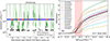 |
Fig. 3. (a): Example using AT 2020vdq to illustrate the calculation of the effective monitoring duration (EMD). Black triangles show the 5σ upper-limit of the CRTS data points, and the green line indicates the maximum LV allowed by the observations as a function of tpeak. Observational time are converted to the phase before the ZTF TDE in the rest-frame. For a given LV (example shown for LV ∼ 1043.14 erg/s, corresponding to MV ∼ −19.4), the time ranges when the maximum allowed LV is below this luminosity (red) are considered effectively monitored, while other times (blue) are not. (b): Resultant EMDs as functions of peak LV for the sample. The dashed black line indicates the average EMD, and the red shaded region marks the typical Lpeak range of SN Ia (−18 < MV < −19.4). |
Finally, we estimated the expected number of SNe that the CRTS could detect in the sample. By adopting the EMD corresponding to MV = −19.4 as an upper limit, we expected a total of < 0.068 SNe Ia. Core-collapse SNE (CCSNe) are less luminous than SNe Ia with a typical MV of > − 18. We estimated the expected number to be ≲0.01 for CCSNe using the EMD for MV = −18. The estimate of CCSNe is highly uncertain due to the large dispersion of Lpeak and the diverse light-curve shapes, which generally differ from those of SNe Ia. Fortunately, it is unlikely that CCSNe dominate the SN detection in our sample, for three reasons. First, the typical 5σ depth of CRTS observations in our sample is MV = −17.9, and only ∼15% of CCSNe at the bright end of the luminosity function are detectable at this depth (e.g. Grayling et al. 2023). Second, only two of the 16 galaxies in our sample are star-forming galaxies with high CCSN rates; the remaining galaxies are passive. Third, both CRTS flares occurred in passive galaxies, with none detected in the two star-forming galaxies.
Assuming a Poisson distribution, the expectation of ≲0.08 yields a probability of only 0.3% for observing at least two flares We rule out the possibility that both flares are caused by SNe given the low probability. Furthermore, the probability that one of the two flares is an SN is only ∼7%, so it is likely that neither of them is an SN.
We examined whether the two CRTS flares could originate in AGN flares (e.g. Graham et al. 2017). Hinkle et al. (2021) studied the pre-flare properties of AT 2019azh’s host galaxy and find it to be a post-starburst galaxy with no AGN features, such as broad emission lines, strong high-ionisation narrow emission lines, and X-ray emission. We also find no evidence for AGN activity in the spectrum and archival X-ray observations of AT 2024pvu3. Additionally, SED fits with CIGALE for both galaxies do not require any AGN component. The MIR colour W1 − W2 is 0.02 ± 0.04 and 0.08 ± 0.04 for AT 2019azh and AT 2024pvu, respectively, consistent with inactive galaxies with W1 − W2 < 0.8 (Stern et al. 2012). Therefore, we exclude the possibility of AGN flares.
3.2. Excessively high TDE rate
In this subsection, we consider the implications for the TDE rate under the assumption that both CRTS flares are TDEs. If we assume that the TDE rate in the galaxies in our sample is the average of M★ ∼ 1010 M⊙ galaxies, 3.2 × 10⁻⁵ galaxy−1 yr−1 (Yao23), even without considering EMD and directly using the duration of CRTS observations (7–8 years), the expected value is only ∼4 × 10⁻³, whereas we actually detected two. Therefore, the TDE rate in this sample is well above average. We then quantitatively calculated the excess of the TDE rate relative to the average value.
We calculated EMDs for the TDEs using the method used in Section 3.1. We assumed GP light curve models as expressed in Eq. (3). To account for the dispersion in the rise and decline timescales of the ZTF TDEs (Yao23), we considered three scenarios for σrise and t0:
-
Slow: σrise = 20 days, t0 = 100 days.
-
Intermediate: σrise = 15 days, t0 = 55 days.
-
Fast: σrise = 10 days, t0 = 35 days.
We show an example of how the maximum Lpeak allowed by the observations varies with tpeak in Figure 4(a), indicating that EMD increases as the TDE evolves more slowly. We list the EMDs for Lpeak = 1043 erg s−1 for each galaxy in Table 1, which range from one to six years for most galaxies.
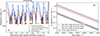 |
Fig. 4. (a): Same example as Figure 3(a), but for TDEs. (b): Luminosity function (LF) of TDEs in our sample, with EMD calculated assuming different timescales (blue, green, and red for fast, intermediate and slow types, respectively). Best estimates are shown as solid lines, while the 1σ upper limit for the fast type and the 1σ lower limit for the slow type are shown as dashed lines. The TDE LF from Yao23 is shown as a shaded grey region for comparison. |
For galaxies in our sample, we assumed a TDE luminosity function (LF) in the form of a single power law (van Velzen 2018; Yao et al. 2023), expressed as
 (7)
(7)
where LV is the peak luminosity of a TDE in the V-band, Ṅ0 is the normalisation in units of  at L0 = 1043erg/s, and γ is the power-law index. Because the two observed flares cannot constrain γ, we fixed γ = 2, consistent with the values of
  obtained for ZTF TDEs by Yao23. We constrained the only free parameter, Ṅ0, with the two observed flares by using the Bayesian method as follows.
First, given the LF, the expected number of TDEs (ETDE) in an infinitesimal interval of dlgLV can be calculated as
 (8)
(8)
where ϕ(lgLV) and teff(lgLV) are the LF and the total EMD of the entire sample at lgLV. We divided the possible lgLV range of 42–45 into bins of width 0.01; using smaller steps produced the same result. For the i-th bin, we calculated the expected number Ei by integrating Eq. (8) over this bin. Meanwhile, the observed lgLV distribution 𝒩 can be expressed as
 (9)
(9)
Then, the probability P(𝒩) for producing the observed distribution 𝒩 can be calculated using the Poisson distribution as
 (10)
(10)
Here, P(𝒩) is a function of the LF normalisation, Ṅ0.
Finally, assuming a logarithmically uniform prior distribution of Ṅ0, we calculated the posterior probability distribution of Ṅ0 using the Bayesian formula
 (11)
(11)
The inferred values of Ṅ0 are  ,
,  , and
, and  × 10−2 galaxy−1 yr−1 dex−1 for the slow, intermediate, and fast types, respectively. We show the resultant LFs in Figure 4(b).
To compare with the average TDE LF from the ZTF, we converted the LF per volume reported by Yao23 to an LF per galaxy. This conversion requires the volume density of galaxies with M★ ∼ 1010 M⊙. Using the galaxy LF of Blanton et al. (2003) derived from z ∼ 0.1 SDSS galaxies, we obtained a volume density of 0.29 − 1.37 × 10⁻² Mpc−3 by integrating with a lower bound of M = −17. Figure 4(b) shows the converted TDE LF in grey, which is two to three orders of magnitude lower than the LF for our sample. This result indicates that, for TDE host galaxies, the probability of another TDE occurring 5–19 years earlier is much higher than the average.
We estimated the fraction of rTDEs with intervals Δt < 20 years in our sample. Table 3 list four rTDEs among the 16 ZTF TDEs, including AT 2019azh and AT 2024pvu with Δt of more than ten years, and AT 2020vdq and AT 2022dbl with Δt ∼ 2 years. Thus, the lower limit of the fraction is ∼25%. The average EMD of CRTS for TDEs with LV = 1043 erg s−1 is 3.2 to 4.3 years, covering 21–29% of the time range of 5–20 years. If we assume that the rTDE rate does not vary with Δt and we ignore multiple repetitions in the same galaxy, we estimate that observations of ≲6 rTDEs were missed. Therefore, we concluded that ∼25 − 60% of optical TDEs are rTDEs. We estimated the rate of rTDEs with Δt < 20 years following Somalwar et al. (2025) by scaling the TDE rate of Yao23:
 (12)
(12)
where 6 yr is the duration of the BTS TDE sample we used. Both the fraction and the rate are higher than those in Somalwar et al. (2025), who only consider Δt < 5 years.
In our sample, there are at least two rTDEs with 5 < Δt < 20 years, considering that more are likely to be missed, while there are only two with Δt < 5 years. Thus, most rTDEs appear to have relatively long time intervals. Previous studies have overlooked this long-interval rTDE population, potentially introducing statistical biases in rTDE research and resulting in an incomplete understanding of their origins.
3.3. Origin of rTDEs
We considered several possible origins of rTDEs and examined whether they could account for the observations in this sample.
3.3.1. Two independent TDEs
We demonstrate in Section 3.2 that, if all rTDEs in the sample are independent TDEs, the inferred TDE rate would be two to three orders of magnitude higher than the average. We examine whether this scenario is feasible.
Post-starburst galaxies, also referred to as green valley galaxies, are known to have a higher TDE rate than the average. AT 2019azh is hosted in a post-starburst galaxy (Hinkle et al. 2021). In addition, the host galaxy of AT 2024pvu has a NUV − r colour of ∼4.5, consistent with green valley galaxies (Schawinski et al. 2014; Belfiore et al. 2018). However, the TDE rate required to account for the rTDEs in these two galaxies remains one to two orders of magnitude higher than the average in post-starburst galaxies.
Theoretical studies suggest that in some post-starburst galaxies, an unequal-mass SMBHB on the verge of merging can increase the TDE rate through the Lidov-Kozai mechanism or three-body scattering by up to several orders of magnitude (Ivanov et al. 2005; Chen et al. 2009). This mechanism is generally considered unlikely to account for the overall high TDE rate in post-starburst galaxies, as this close SMBHB stage lasts only approximately 105 years (e.g., Stone et al. 2020). However, the host galaxies of the rTDE in our sample may be in this stage and have an extremely high TDE rate of ∼ 10−2 galaxy−1 yr−1 (Liu & Chen 2013). A close SMBH companion could potentially be detected using the gap in the TDE’s X-ray light curve, which arises from its gravitational disturbance of the TDE debris fallback stream (Liu et al. 2014; Shu et al. 2020). Although no such gap was observed in the X-ray monitoring of AT 2019azh (Hinkle et al. 2021), we cannot rule out its existence, as the current X-ray coverage is insufficient.
The TDE rate decreases with increasing SMBH mass, MBH, and is heavily suppressed at MBH ≳ 108 M⊙, which is the Hills mass for Sun-like stars (e.g. van Velzen 2018; Polkas et al. 2024; Hannah et al. 2025). We adopted MBH= 106.44 for AT 2019azh from Hinkle et al. (2021) and estimate MBH ∼ 107.9 M⊙ using the Mbulge − MBH correlation of McConnell & Ma (2013). For such a high MBH, even with a companion SMBH to increase the TDE rate, a considerable fraction of TDEs would not be observed as flares because the star falls into the event horizon before being tidally disrupted. Thus, the high MBH disfavors the scenario of independent TDEs for AT 2024pvu.
3.3.2. Repeating partial TDEs
We considered the scenario of repeating partial TDEs, which is proposed to explain periodic TDE-like flares, such as ASASSN-14ko, eRASSt J045650.3–203750, and AT 2023uqm. In this model, the star moves in a highly eccentric orbit around an SMBH, with Rp allowing for a partial TDE (∼1 − 2 Rt for a fractional mass loss ≳10%, Ryu et al. 2020a,b) and triggers a flare each time it passes the periapsis. Adopting the observed intervals in AT 2019azh and AT 2024pvu as the orbiting periods, we estimate a to be 780 and 2850 AU using MBH and Kepler’s third law. Assuming Sun-like stars, Rt is 0.65 and 2.0 AU for AT 2019azh and AT 2024pvu, respectively. Assuming Rp = a(1 − e)≈1 − 2 Rt, we estimate 1 − e ≈ 10−3 for both rTDEs.
In the rpTDE model, the series of flares produced by the star should be regarded as a single event. We now assess the impact this has on the optical TDE event rate.
We first estimated the average number of flares ( ) produced by each rpTDE. At present, we cannot measure
  directly through observations in our sample. We considered two possible ranges of
  : a few, as in eRASSt J045650.3–203750 (5), and several dozen, as in ASASSN-14ko (> 30). The former scenario requires a fractional mass loss of ≳10%, whereas the latter requires ≲5%. We favour the former for the following reasons. First, the energies of the flare in our sample can vary by several factors (Table 3), which does not match the situation in ASASSN-14ko, where the flare energies are similar. In the rpTDE model, the flare energies may vary significantly due to variations in the stellar structure. For example, a decrease in stellar density after a pTDE may increase the fractional mass loss of the next pTDE, or even lead to a full TDE (e.g. Liu et al. 2025). Therefore, observing significant variations in flare energy may indicate that a series of rpTDEs is ending, supporting a lower number of repetitions. Second, the average flare energy in our sample is of the order of 1051 erg (Table 3), which is higher than that of ASASSN-14ko (∼1050 erg; (Huang et al. 2025)) and comparable to typical values in the ZTF TDE sample (van Velzen et al. 2021; Yao et al. 2023). It would be more reasonable to assume
  of several, because
  of several dozen requires disruptions of large-mass stars with low probability. Finally, for AT 2020vdq and AT 2022dbl, Somalwar et al. (2025) and Lin et al. (2024) found no earlier flares before the ZTF detection, implying that the observed flare is the first in the series. Such a scenario would be highly improbable if
  were several dozen. Therefore, it is reasonable to assume
  of a few for rpTDEs.
Properties of rTDEs in the sample.
An rpTDE is more likely to fall within a time-limited sample than a single TDE. This selection effect can lead to an overestimation of the TDE rate and the rpTDE fraction. There are a total of 18 ZTF flares in our sample, considering that AT 2020vdq and AT 2022dbl each contributed two flares. We assume that approximately six to 12 of them were produced by rpTDEs and the remaining six to 12 were produced by single TDEs. By dividing the former by  , which is assumed to be three to ten, we estimate the correction factor for the optical TDE rate to be 40 − 80% (∼ 2 × 10⁻⁵ galaxy−1 yr−1, using the observed ZTF value; Yao23), and the fraction of rpTDEs to be ∼5 − 40%. If we include rpTDEs with periods ≳20 years, the TDE rate decreases further, while the fraction of rpTDEs increases.
Mechanisms are required to send stars onto highly eccentric orbits with 1 − e ≈ 10−3. A widely accepted mechanism involves a close stellar binary system being tidally dissociated as it approaches the SMBH, with one star escaping and the other captured into a highly eccentric orbit (Hills 1988). The binary must be tight, with separation abin ≲ 10 R⊙, to survive stellar scattering in the galactic nucleus (e.g., Hills 1988). The semi-major axis of the captured star is primarily related to abin (Cufari et al. 2022), which is roughly
 (13)
(13)
This correlation shows a scatter of 0.5–2 according to simulations (Yu & Lai 2024). Assuming M★ = M⊙, the inferred abin is ∼17 for AT 2019azh and ∼7 R⊙ for AT 2024pvu. This is roughly in line with the close-binary condition, taking into account the scatter of the correlation, the measurement error of MBH, and the uncertainty of M★.
For a close binary, the Rp of the captured star is approximately equal to the Rp of the original binary’s centre of mass. A natural interpretation of rpTDE is that this initial Rp permits partial disruption of the captured star (Rp ≲ 2 Rt). In this scenario, the first pTDE occurs when the binary system passes through periapsis before dissociating. Both stars may undergo pTDE, but only one flare would be observed because the time interval is short. Subsequently, each return of the captured star to periapsis triggers a flare, continuing until the star is fully disrupted or only an unbreakable core remains.
We now examine whether the observed rpTDE fraction of ∼5 − 40% can be explained within this framework. To estimate the proportions of different types of TDEs, we considered only single stars and close binaries, as wide binaries in the galactic nucleus would transform into either single stars or close binaries after scattering with fellow stars. We assumed that rpTDE can occur in close binaries with Rp that allows partial TDE, whereas a single TDE occurs in single stars or in close binaries with Rp that allows full TDEs. According to loss cone theory, the event rate of partial TDEs is roughly twice that of full TDEs (Stone et al. 2020), so the fraction of Rp that satisfies the condition for partial TDE is approximately two-thirds. Consequently, the observed rpTDE fraction further requires a fraction of close binaries among all stars, roughly fclose ∼ 7 − 60%. This fraction is much higher than that observed in nearby open star clusters, which is only ≲2% (abin ≲ 10 R⊙, e.g. Patience et al. 2002). Recent theoretical studies show that in galactic nuclei, gravitational perturbations from the SMBH and flyby stars can convert ∼20 − 50% of wide binaries into close binaries (Dodici et al. 2025; Hao-Tse Huang & Lu 2025). Assuming an initial binary fraction of ∼40 − 60% (e.g. Duchêne & Kraus 2013), these effects may increase fclose to ∼10 − 30%, meeting the requirement to explain rpTDEs using the Hills mechanism. This high fraction further predicts a large number of eclipsing binaries in the galactic nucleus, which can be tested observationally through infrared time-domain surveys.
Another way to enhance the rpTDE rate in the Hills mechanism is to consider a larger Rp of the binary’s centre of mass. The star is captured with Rp > 2Rt initially, with no partial TDE occurring. After orbiting for a period of time, Rp decreases or Rt increases, and a partial TDE can occur. The Rt of the captured star can increase through tidal heating and tidal spin-up (Liu et al. 2025). In addition, the Rp of the captured star can decrease under gravitational perturbation of the nuclear cluster on a timescale of ∼107 − 109 years, while a remains almost unchanged (Pan & Lai 2026). However, quantitative predictions of how much Rt can increase or Rp can decrease require further detailed numerical simulations.
Beyond the Hills mechanism, highly eccentric orbits can also arise from the scattering within the S-star cluster (Bromley et al. 2012), including both internal scattering and scattering with intruding stars. If AT 2019azh and AT 2024pvu are rpTDEs formed via this channel, the scattering position has a distance of ∼103 AU, coinciding with the inner edge of the S cluster in the Milky Way (Eckart & Genzel 1996). However, the S cluster in the Milky Way is not sufficiently dense to generate a large number of rpTDEs (Alexander 2017). Recently, Jiang & Pan (2025) proposed a model for interpreting QPE observed years after a TDE occurs, involving a collision between a pre-existing orbiting star and the newly formed TDE disc. This model suggests exceptionally abundant stars in the vicinity of SMBH, which can be explained as a result of a recently faded AGN, where stars were captured by the AGN accretion disc (Pan & Yang 2021) or formed in the disc in situ (Fan & Wu 2023). Stars in such rich stellar discs may fall towards the SMBH on highly eccentric orbits through stellar scattering or the gravitational perturbation of a massive object, such as a companion SMBH. The rpTDEs formed in this channel would have semi-major axes of ∼103 − 104 Rg, comparable to the size of the AGN outer disc and consistent with the observations of our sample. However, whether this mechanism can account for the observed rTDE rate requires further investigation.
3.3.3. Other possibilities and future observational tests
Since only two flares have been detected for the rTDEs in our sample, we considered ‘double TDEs’ formed by sequential tidal disruptions of binary stars when they encounter the SMBH (e.g. Mandel & Levin 2015; Yu & Lai 2024). For typical parameters, the time interval between two TDEs does not exceed several months, and the combined light curve would be similar to that of non-repetitive TDEs. Double TDEs produced by SMBHB can have time intervals of up to several decades (e.g. Coughlin et al. 2018; Wu & Yuan 2018). However, the probability of a long interval (> 10 years) is less than 1%, which cannot explain the high observed fraction of rTDEs. Therefore, we exclude double TDEs as the origin of rTDEs in our sample.
In summary, we favour the rpTDE model to explain the rTDEs in our sample, although we cannot rule out the possibility of independent TDEs. The rpTDE model predicts that rTDEs are periodic, which requires verification through future observations. In November 2025, a new flare was detected in IC 3599 (Grupe et al. 2025), potentially part of a series of TDEs with a period of ∼18 years, in addition to the two previously detected flares. Follow-up observations of IC 3599 may provide conclusive evidence for the existence of rTDEs with periods exceeding ten years. The independent TDE model predicts that the time intervals between rTDEs are uniformly distributed. This could not be tested with the current small sample due to large statistical uncertainties and will require larger rTDE samples in the future.
4. Summary
Using CRTS data, we performed a systematic search for rTDEs with intervals of 5–19 years in a sample of 16 ZTF BTS TDEs at z < 0.05. Using a ‘consecutive > 5σ excess’ threshold, we identified two CRTS flares in the host galaxies of AT 2019azh and AT 2024pvu. The peak V-band luminosities, lgLV,peak, of the CRTS flares are  and 43.25 ± 0.05, comparable to those of the ZTF flares, with rest-frame intervals of 13.2 and 17.1 years.
AT 2024pvu.I was serendipitously observed by GALEX in the FUV and NUV bands near the peak. The flare was detected in both bands, with UV fluxes two orders of magnitude higher than the host galaxy’s contribution, inferred from Swift/UVOT data and optical-to-IR SED data. The flare’s UV and optical SED can be well described by a blackbody with a temperature of ∼19 500 K, much higher than those of SNe and consistent with those of TDEs.
We also estimated the expected number of SNe in the sample. First, we predicted the rates of SNe Ia and CCSNe in the sample based on the stellar masses and star formation rates of the galaxies. We then calculated the EMDs for the CRTS observations by assuming typical SN light curves. We find average EMDs of 2.27 and 0.28 years for peak MV of −19.4 and −18, respectively. The expected number of SNe Ia in all 16 galaxies is < 0.068, and that of CCSNe is ≲0.01. With a total expected number of ≲0.08, the probability that both flares are due to SN is only 0.3%. Thus, AT 2019azh and AT 2024pvu are likely rTDEs.
Given that the average EMD of CRTS observations for TDEs is only 2.7–4.9 years, detecting two TDEs in 16 galaxies indicates an exceptionally high TDE rate 5–19 years prior to the ZTF TDEs in this sample. Assuming a power-law LF, we estimate that the TDE rate is two to three orders of magnitude higher than the average. The fraction of rTDEs in the TDE sample is also high: including two additional rTDEs identified by the ZTF with intervals of ∼2 years (AT 2020vdq and AT 2022dbl), at least four of the 16 rTDEs are repeating. Taking into account possible rTDEs missed by the CRTS, we estimate the fraction of rTDEs with time intervals shorter than 20 years to be ∼25%−60%.
We propose two interpretations for the high rTDE fraction. The first is that the two TDEs are independent, and the TDE rate in the galaxies in this sample was boosted by two to three orders of magnitude by a parsec-scale SMBH companion. The second is that both AT 2019azh and AT 2024pvu are rpTDEs from a star on a highly eccentric (1 − e ∼ 10−3) orbit. In this scenario, the observed optical TDE rate is overestimated. Assuming an average of several flares per rpTDE, we estimate a correction factor for the rate of ∼40 − 80%. We favour the rpTDE interpretation. However, the channel through which the star enters such an orbit remains unclear. It could result from the Hills mechanism or scattering within an ultradense stellar disc left by a faded AGN. We present predictions for each interpretation, which require future observational tests.
Acknowledgments
We thank the anonymous reviewer for helping to improve the manuscript. We thank Zhen Pan for thoughtful suggestions on explaining the formations of rpTDEs. This work is supported by the National Natural Science Foundation of China (NFSC, 12103002) and the University Annual Scientific Research Plan of Anhui Province (2022AH010013). The CSS survey is funded by the National Aeronautics and Space Administration under Grant No. NNG05GF22G issued through the Science Mission Directorate Near-Earth Objects Observations Program. The CRTS survey is supported by the U.S. National Science Foundation under grants AST-0909182. The ZTF are supported by the National Science Foundation under Grants No. AST-1440341 and AST-2034437 and a collaboration including current partners Caltech, IPAC, the Oskar Klein Center at Stockholm University, the University of Maryland, University of California, Berkeley, the University of Wisconsin at Milwaukee, University of Warwick, Ruhr University, Cornell University, Northwestern University and Drexel University. Operations are conducted by Caltech’s Optical Observatory (COO), Caltech/IPAC and the University of Washington at Seattle (UW). We thank the Swift science operations team for accepting our ToO requests and arranging the observations. This work made use of data supplied by the UK Swift Science Data Centre (UKSSDC) at the University of Leicester.
References
- Alexander, T. 2017, ARA&A, 55, 17 [NASA ADS] [CrossRef] [Google Scholar]
- Arcavi, I., Gal-Yam, A., Sullivan, M., et al. 2014, ApJ, 793, 38 [Google Scholar]
- Astropy Collaboration (Price-Whelan, A. M., et al.) 2022, ApJ, 935, 20 [CrossRef] [Google Scholar]
- Bao, D.-W., Guo, W.-J., Zhang, Z.-X., et al. 2024, ApJ, 977, 279 [Google Scholar]
- Belfiore, F., Maiolino, R., Bundy, K., et al. 2018, MNRAS, 477, 3014 [Google Scholar]
- Bellm, E. C., Kulkarni, S. R., Graham, M. J., et al. 2019, PASP, 131, 018002 [Google Scholar]
- Blanton, M. R., Hogg, D. W., Bahcall, N. A., et al. 2003, ApJ, 592, 819 [Google Scholar]
- Boquien, M., Burgarella, D., Roehlly, Y., et al. 2019, A&A, 622, A103 [NASA ADS] [CrossRef] [EDP Sciences] [Google Scholar]
- Botticella, M. T., Smartt, S. J., Kennicutt, R. C., et al. 2012, A&A, 537, A132 [NASA ADS] [CrossRef] [EDP Sciences] [Google Scholar]
- Bradley, L., Sipőcz, B., Robitaille, T., et al. 2025, https://doi.org/10.5281/zenodo.14889440 [Google Scholar]
- Brandt, W. N., Pounds, K. A., & Fink, H. 1995, MNRAS, 273, L47 [Google Scholar]
- Bromley, B. C., Kenyon, S. J., Geller, M. J., & Brown, W. R. 2012, ApJ, 749, L42 [NASA ADS] [CrossRef] [Google Scholar]
- Bruzual, G., & Charlot, S. 2003, MNRAS, 344, 1000 [NASA ADS] [CrossRef] [Google Scholar]
- Calzetti, D., Armus, L., Bohlin, R. C., et al. 2000, ApJ, 533, 682 [NASA ADS] [CrossRef] [Google Scholar]
- Campana, S., Mainetti, D., Colpi, M., et al. 2015, A&A, 581, A17 [NASA ADS] [CrossRef] [EDP Sciences] [Google Scholar]
- Chambers, K. C., Magnier, E. A., Metcalfe, N., et al. 2016, arXiv e-prints [arXiv:1612.05560] [Google Scholar]
- Chang, J. N. Y., Dai, L., Pfister, H., Kar Chowdhury, R., & Natarajan, P. 2025, ApJ, 980, L22 [Google Scholar]
- Chen, X., Madau, P., Sesana, A., & Liu, F. K. 2009, ApJ, 697, L149 [NASA ADS] [CrossRef] [Google Scholar]
- Coughlin, E. R., & Nixon, C. J. 2019, ApJ, 883, L17 [NASA ADS] [CrossRef] [Google Scholar]
- Coughlin, E. R., Darbha, S., Kasen, D., & Quataert, E. 2018, ApJ, 863, L24 [NASA ADS] [CrossRef] [Google Scholar]
- Cufari, M., Coughlin, E. R., & Nixon, C. J. 2022, ApJ, 929, L20 [NASA ADS] [CrossRef] [Google Scholar]
- Dale, D. A., Helou, G., Magdis, G. E., et al. 2014, ApJ, 784, 83 [Google Scholar]
- Desai, D. D., Kochanek, C. S., Shappee, B. J., et al. 2024, MNRAS, 530, 5016 [NASA ADS] [CrossRef] [Google Scholar]
- Dodici, M., Tremaine, S., & Wu, Y. 2025, arXiv e-prints [arXiv:2511.02905] [Google Scholar]
- Drake, A. J., Djorgovski, S. G., Mahabal, A., et al. 2009, ApJ, 696, 870 [Google Scholar]
- Drake, A. J., Catelan, M., Djorgovski, S. G., et al. 2013, ApJ, 763, 32 [NASA ADS] [CrossRef] [Google Scholar]
- Duchêne, G., & Kraus, A. 2013, ARA&A, 51, 269 [Google Scholar]
- Eckart, A., & Genzel, R. 1996, Nature, 383, 415 [NASA ADS] [CrossRef] [Google Scholar]
- Fan, X., & Wu, Q. 2023, ApJ, 944, 159 [NASA ADS] [CrossRef] [Google Scholar]
- Fitzpatrick, E. L. 1999, PASP, 111, 63 [Google Scholar]
- Foreman-Mackey, D., Hogg, D. W., Lang, D., & Goodman, J. 2013, PASP, 125, 925 [Google Scholar]
- Frank, J., & Rees, M. J. 1976, MNRAS, 176, 633 [NASA ADS] [CrossRef] [Google Scholar]
- Fremling, C., Miller, A. A., Sharma, Y., et al. 2020, ApJ, 895, 32 [NASA ADS] [CrossRef] [Google Scholar]
- French, K. D., Arcavi, I., & Zabludoff, A. 2016, ApJ, 818, L21 [NASA ADS] [CrossRef] [Google Scholar]
- Gezari, S. 2021, ARA&A, 59, 21 [NASA ADS] [CrossRef] [Google Scholar]
- Ginsburg, A., Sipőcz, B. M., Brasseur, C. E., et al. 2019, AJ, 157, 98 [Google Scholar]
- Gordon, K. 2024, J. Open Source Software, 9, 7023 [Google Scholar]
- Gordon, K. D., Clayton, G. C., Decleir, M., et al. 2023, ApJ, 950, 86 [CrossRef] [Google Scholar]
- Graham, M. J., Djorgovski, S. G., Drake, A. J., et al. 2017, MNRAS, 470, 4112 [NASA ADS] [CrossRef] [Google Scholar]
- Grayling, M., Gutiérrez, C. P., Sullivan, M., et al. 2023, MNRAS, 520, 684 [CrossRef] [Google Scholar]
- Grotova, I., Rau, A., Baldini, P., et al. 2025, A&A, 697, A159 [NASA ADS] [CrossRef] [EDP Sciences] [Google Scholar]
- Grupe, D., Beuermann, K., Mannheim, K., et al. 1995, A&A, 299, L5 [NASA ADS] [Google Scholar]
- Grupe, D., Komossa, S., & Saxton, R. 2015, ApJ, 803, L28 [NASA ADS] [CrossRef] [Google Scholar]
- Grupe, D., Komossa, S., Wolsing, S., & Schartel, N. 2025, ATel, 17479, 1 [Google Scholar]
- Hammerstein, E., van Velzen, S., Gezari, S., et al. 2023, ApJ, 942, 9 [NASA ADS] [CrossRef] [Google Scholar]
- Hannah, C. H., Stone, N. C., Seth, A. C., & van Velzen, S. 2025, ApJ, 988, 29 [Google Scholar]
- Hao-Tse Huang, H., & Lu, W. 2025, arXiv e-prints [arXiv:2511.11965] [Google Scholar]
- Hills, J. G. 1975, Nature, 254, 295 [Google Scholar]
- Hills, J. G. 1988, Nature, 331, 687 [Google Scholar]
- Hinkle, J. T., Holoien, T. W.-S., Auchettl, K., et al. 2021, MNRAS, 500, 1673 [Google Scholar]
- Hinkle, J. T., Auchettl, K., Hoogendam, W. B., et al. 2024, arXiv e-prints [arXiv:2412.15326] [Google Scholar]
- Hodgkin, S. T., Harrison, D. L., Breedt, E., et al. 2021, A&A, 652, A76 [NASA ADS] [CrossRef] [EDP Sciences] [Google Scholar]
- Hoogendam, W. B., Hinkle, J. T., Shappee, B. J., et al. 2024, MNRAS, 530, 4501 [NASA ADS] [CrossRef] [Google Scholar]
- Huang, S., Wang, T., Jiang, N., et al. 2025, ApJ, 988, 237 [Google Scholar]
- Ivanov, P. B., Polnarev, A. G., & Saha, P. 2005, MNRAS, 358, 1361 [Google Scholar]
- Ji, S., Wang, Z., Zhu, L., Geier, S., & Gupta, A. C. 2025, ApJ, 991, 20 [Google Scholar]
- Jiang, N., & Pan, Z. 2025, ApJ, 983, L18 [Google Scholar]
- Jiang, N., Wang, T., Dou, L., et al. 2021, ApJS, 252, 32 [Google Scholar]
- Kochanek, C. S., Shappee, B. J., Stanek, K. Z., et al. 2017, PASP, 129, 104502 [Google Scholar]
- Komossa, S. 2015, J. High Energy Astrophys., 7, 148 [Google Scholar]
- Langis, D. A., Liodakis, I., Koljonen, K. I. I., et al. 2026, A&A, 707, A171 [NASA ADS] [CrossRef] [EDP Sciences] [Google Scholar]
- Law-Smith, J., Ramirez-Ruiz, E., Ellison, S. L., & Foley, R. J. 2017, ApJ, 850, 22 [Google Scholar]
- Li, W., Leaman, J., Chornock, R., et al. 2011, MNRAS, 412, 1441 [NASA ADS] [CrossRef] [Google Scholar]
- Lin, Z., Jiang, N., Wang, T., et al. 2024, ApJ, 971, L26 [NASA ADS] [CrossRef] [Google Scholar]
- Liu, F. K., & Chen, X. 2013, ApJ, 767, 18 [Google Scholar]
- Liu, F. K., Li, S., & Komossa, S. 2014, ApJ, 786, 103 [Google Scholar]
- Liu, Z., Malyali, A., Krumpe, M., et al. 2023, A&A, 669, A75 [NASA ADS] [CrossRef] [EDP Sciences] [Google Scholar]
- Liu, Z., Ryu, T., Goodwin, A. J., et al. 2024, A&A, 683, L13 [NASA ADS] [CrossRef] [EDP Sciences] [Google Scholar]
- Liu, C., Yarza, R., & Ramirez-Ruiz, E. 2025, ApJ, 979, 40 [Google Scholar]
- Makrygianni, L., Arcavi, I., Newsome, M., et al. 2025, ApJ, 987, L20 [Google Scholar]
- Mandel, I., & Levin, Y. 2015, ApJ, 805, L4 [Google Scholar]
- Martin, D. C., Fanson, J., Schiminovich, D., et al. 2005, ApJ, 619, L1 [Google Scholar]
- Masci, F. J., Laher, R. R., Rusholme, B., et al. 2019, PASP, 131, 018003 [Google Scholar]
- Masterson, M., De, K., Panagiotou, C., et al. 2024, ApJ, 961, 211 [NASA ADS] [CrossRef] [Google Scholar]
- McConnell, N. J., & Ma, C.-P. 2013, ApJ, 764, 184 [Google Scholar]
- Merritt, D. 2013, Class. Quant. Grav., 30, 244005 [NASA ADS] [CrossRef] [Google Scholar]
- Miles, P. R., Coughlin, E. R., & Nixon, C. J. 2020, ApJ, 899, 36 [NASA ADS] [CrossRef] [Google Scholar]
- Mockler, B., Hammerstein, E., Coughlin, E. R., & Nicholl, M. 2026, Encycl. Astrophys., 3, 423 [Google Scholar]
- Pan, Z., & Lai, D. 2026, arXiv e-prints [arXiv:2601.22465] [Google Scholar]
- Pan, Z., & Yang, H. 2021, Phys. Rev. D, 103, 103018 [CrossRef] [Google Scholar]
- Patience, J., Ghez, A. M., Reid, I. N., & Matthews, K. 2002, AJ, 123, 1570 [NASA ADS] [CrossRef] [Google Scholar]
- Payne, A. V., Shappee, B. J., Hinkle, J. T., et al. 2021, ApJ, 910, 125 [NASA ADS] [CrossRef] [Google Scholar]
- Payne, A. V., Shappee, B. J., Hinkle, J. T., et al. 2022, ApJ, 926, 142 [NASA ADS] [CrossRef] [Google Scholar]
- Payne, A. V., Auchettl, K., Shappee, B. J., et al. 2023, ApJ, 951, 134 [NASA ADS] [CrossRef] [Google Scholar]
- Perley, D. A., Fremling, C., Sollerman, J., et al. 2020, ApJ, 904, 35 [NASA ADS] [CrossRef] [Google Scholar]
- Polkas, M., Bonoli, S., Bortolas, E., et al. 2024, A&A, 689, A204 [NASA ADS] [CrossRef] [EDP Sciences] [Google Scholar]
- Predehl, P., Andritschke, R., Arefiev, V., et al. 2021, A&A, 647, A1 [EDP Sciences] [Google Scholar]
- Rees, M. J. 1988, Nature, 333, 523 [Google Scholar]
- Rehemtulla, N., Miller, A. A., Jegou Du Laz, T., et al. 2024, ApJ, 972, 7 [Google Scholar]
- Roming, P. W. A., Kennedy, T. E., Mason, K. O., et al. 2005, Space Sci. Rev., 120, 95 [Google Scholar]
- Ryu, T., Krolik, J., Piran, T., & Noble, S. C. 2020a, ApJ, 904, 98 [NASA ADS] [CrossRef] [Google Scholar]
- Ryu, T., Krolik, J., Piran, T., & Noble, S. C. 2020b, ApJ, 904, 100 [NASA ADS] [CrossRef] [Google Scholar]
- Salpeter, E. E. 1955, ApJ, 121, 161 [Google Scholar]
- Saxton, R. D., Motta, S. E., Komossa, S., & Read, A. M. 2015, MNRAS, 454, 2798 [NASA ADS] [CrossRef] [Google Scholar]
- Saxton, R., Komossa, S., Auchettl, K., & Jonker, P. G. 2020, Space Sci. Rev., 216, 85 [NASA ADS] [CrossRef] [Google Scholar]
- Sazonov, S., Gilfanov, M., Medvedev, P., et al. 2021, MNRAS, 508, 3820 [NASA ADS] [CrossRef] [Google Scholar]
- Schawinski, K., Urry, C. M., Simmons, B. D., et al. 2014, MNRAS, 440, 889 [Google Scholar]
- Shappee, B. J., Prieto, J. L., Grupe, D., et al. 2014, ApJ, 788, 48 [Google Scholar]
- Shingles, L., Smith, K. W., Young, D. R., et al. 2021, Transient Name Server AstroNote, 7, 1 [NASA ADS] [Google Scholar]
- Shu, X., Zhang, W., Li, S., et al. 2020, Nat. Commun., 11, 5876 [NASA ADS] [CrossRef] [Google Scholar]
- Skrutskie, M. F., Cutri, R. M., Stiening, R., et al. 2006, AJ, 131, 1163 [NASA ADS] [CrossRef] [Google Scholar]
- Smith, M., Nichol, R. C., Dilday, B., et al. 2012, ApJ, 755, 61 [Google Scholar]
- Smith, K. W., Smartt, S. J., Young, D. R., et al. 2020, PASP, 132, 085002 [Google Scholar]
- Somalwar, J. J., Ravi, V., Yao, Y., et al. 2025, ApJ, 985, 175 [Google Scholar]
- Stein, R., Ahumada, T., Angus, C., et al. 2024, Transient Name Server AstroNote, 221, 1 [Google Scholar]
- Stern, D., Assef, R. J., Benford, D. J., et al. 2012, ApJ, 753, 30 [Google Scholar]
- Stone, N. C., & Metzger, B. D. 2016, MNRAS, 455, 859 [NASA ADS] [CrossRef] [Google Scholar]
- Stone, N. C., Vasiliev, E., Kesden, M., et al. 2020, Space Sci. Rev., 216, 35 [NASA ADS] [CrossRef] [Google Scholar]
- Strovink, M. 2007, ApJ, 671, 1084 [Google Scholar]
- Sun, L., Jiang, N., Dou, L., et al. 2024, A&A, 692, A262 [NASA ADS] [CrossRef] [EDP Sciences] [Google Scholar]
- Sun, J., Guo, H., Gu, M., et al. 2025, ApJ, 982, 150 [Google Scholar]
- Tonry, J. L., Denneau, L., Heinze, A. N., et al. 2018, PASP, 130, 064505 [Google Scholar]
- van Velzen, S. 2018, ApJ, 852, 72 [NASA ADS] [CrossRef] [Google Scholar]
- van Velzen, S., Holoien, T. W.-S., Onori, F., Hung, T., & Arcavi, I. 2020, Space Sci. Rev., 216, 124 [CrossRef] [Google Scholar]
- van Velzen, S., Gezari, S., Hammerstein, E., et al. 2021, ApJ, 908, 4 [NASA ADS] [CrossRef] [Google Scholar]
- Wang, J., & Merritt, D. 2004, ApJ, 600, 149 [NASA ADS] [CrossRef] [Google Scholar]
- Wang, Y., Wang, T., Huang, S., et al. 2025, arXiv e-prints [arXiv:2510.26561] [Google Scholar]
- Wevers, T., Coughlin, E. R., Pasham, D. R., et al. 2023, ApJ, 942, L33 [NASA ADS] [CrossRef] [Google Scholar]
- Wright, E. L., Eisenhardt, P. R. M., Mainzer, A. K., et al. 2010, AJ, 140, 1868 [Google Scholar]
- Wu, X.-J., & Yuan, Y.-F. 2018, MNRAS, 479, 1569 [NASA ADS] [CrossRef] [Google Scholar]
- Yao, Y., Ravi, V., Gezari, S., et al. 2023, ApJ, 955, L6 [NASA ADS] [CrossRef] [Google Scholar]
- Yao, Y., Guolo, M., Tombesi, F., et al. 2024, ApJ, 976, 34 [Google Scholar]
- Yao, Y., Chornock, R., Ward, C., et al. 2025a, ApJ, 985, L48 [Google Scholar]
- Yao, Y., Ye, J., Sun, L., et al. 2025b, ApJS, 281, 7 [Google Scholar]
- York, D. G., Adelman, J., Anderson, J. E., Jr, et al. 2000, AJ, 120, 1579 [Google Scholar]
- Yu, F., & Lai, D. 2024, ApJ, 977, 268 [Google Scholar]
- Zabludoff, A., Arcavi, I., LaMassa, S., et al. 2021, Space Sci. Rev., 217, 54 [NASA ADS] [CrossRef] [Google Scholar]
- Zhang, Z., Yao, Y., Gilfanov, M., et al. 2026, A&A, 708, A374 [NASA ADS] [CrossRef] [EDP Sciences] [Google Scholar]
- Zhu, J., Jiang, N., Wang, T., et al. 2023, ApJ, 952, L35 [NASA ADS] [CrossRef] [Google Scholar]
We selected 71 TDEs before July 1, 2025; https://sites.astro.caltech.edu/ztf/bts/bts.php
We will present a detailed analysis in a future work.
Appendix A: Data collection and reduction
A.1. Milky Way galactic extinction
For all the photometric data, we corrected for galactic extinction using python package dust_extinction (Gordon 2024). We adopted Av values from the BTS catalogue, and used models from Fitzpatrick (1999) and Gordon et al. (2023) for UV bands and other bands, respectively.
A.2. Light curve data
Here we briefly introduce how we collected and reduced the light curve data other than CRTS, including ASASSN, Gaia, ATLAS, ZTF and Swift UVOT.
We obtained ASASSN light curves of AT 2019azh and AT 2024pvu in V and g bands from the website4 generated using image subtraction photometry. Due to the larger flux error of ASASSN, we binned the data weekly.
We obtained the Gaia space telescope (Gaia; Hodgkin et al. 2021) G-band light curve of AT 2019azh from the alert system5. The Gaia alert system does not provide magnitude error. However, AT 2019azh has G ∼ 17 and the typical magnitude error is < 0.05 mag, ensuring the accuracy of the photometry.
We obtained the ATLAS light curves in c and o bands from the forced photometry server6. We selected photometry on the difference images. We removed data taken under bad weather (limit magnitude < 19), and binned the light curve nightly.
We obtained the ZTF light curves in g and r bands from the NASA/IPAC infrared science archive7 (IRSA). We removed bad data points using observational logs following the ZTF Science Data System explanatory supplement. We subtracted the host flux using the median of the quiescent fluxes.
We downloaded the Swift UVOT data of AT 2024pvu from the NASA’s Archive of Data on Energetic Phenomena8. We made photometry on the UVOT images using uvotsource in High Energy Astrophysics Software. We used an aperture with a radius of 5″, and calculated the background in two nearby circular regions without a source.
A.3. SED data
We collected the SED data of the whole galaxy as follows.
We obtained the GALEX photometries in the FUV and NUV bands from the Mikulski Archive for Space Telescopes9. We also downloaded the GALEX images of AT 2024pvu from the same archive.
We queried photometries from SDSS in the u, g, r, i and z bands using python package astroquery (Ginsburg et al. 2019), and selected model magnitudes. For some galaxies that were not observed by SDSS, we collected the photometries from the Panoramic Survey Telescope and Rapid Response System (PanSTARRS; Chambers et al. 2016) in the g, r, i, z, and y bands from the source catalogue10, and selected the mean Kron aperture magnitudes.
We obtained the photometries of 2MASS in the J, H, and K bands and WISE in the W1 to W4 bands through IRSA. We adopted the 2MASS magnitudes in the extended source catalogue if available; otherwise, we did not use 2MASS data in the SED fitting because the photometries in the point source catalogue underestimate the whole galaxy’s flux. For the WISE magnitudes, we checked whether the pipeline identified the galaxy as a point source (ext_flg = 0). If so, we adopted the magnitudes in the catalogue from profile fitting. Otherwise, i.e. the galaxy should be treated as an extended source, we measured Kron aperture fluxes on the WISE images using the python code photutils (Bradley et al. 2025), instead of using the magnitudes in the catalogue.
All Tables
All Figures
|
Fig. 1. Host-subtracted optical light curves of AT 2019azh and AT 2024pvu. Insert panels show zoomed views of the CRTS flares and the Gaussian+Power-law (GP) models that fit the data. For AT 2024pvu, the observation time of GALEX is indicated by a dashed green line. |
| In the text | |
|
Fig. 2. (a): Spectral energy distribution (SED) of AT 2024pvu from UV to MIR. Blue points represent the host galaxy SED in the quiescent state. The black line indicates the best-fitting model from CIGALE with the minimum χ2. We show GALEX and Swift UV photometries as red pentagrams and red triangles, respectively. The SWIFT measurement agrees with the CIGALE prediction (open black circle with error bar), whereas the GALEX measurement shows a significant excess. (b): Spectral energy distribution (SED) of the CRTS flare at the time of the GALEX observation, with blackbody models fitted using MCMC. |
| In the text | |
|
Fig. 3. (a): Example using AT 2020vdq to illustrate the calculation of the effective monitoring duration (EMD). Black triangles show the 5σ upper-limit of the CRTS data points, and the green line indicates the maximum LV allowed by the observations as a function of tpeak. Observational time are converted to the phase before the ZTF TDE in the rest-frame. For a given LV (example shown for LV ∼ 1043.14 erg/s, corresponding to MV ∼ −19.4), the time ranges when the maximum allowed LV is below this luminosity (red) are considered effectively monitored, while other times (blue) are not. (b): Resultant EMDs as functions of peak LV for the sample. The dashed black line indicates the average EMD, and the red shaded region marks the typical Lpeak range of SN Ia (−18 < MV < −19.4). |
| In the text | |
|
Fig. 4. (a): Same example as Figure 3(a), but for TDEs. (b): Luminosity function (LF) of TDEs in our sample, with EMD calculated assuming different timescales (blue, green, and red for fast, intermediate and slow types, respectively). Best estimates are shown as solid lines, while the 1σ upper limit for the fast type and the 1σ lower limit for the slow type are shown as dashed lines. The TDE LF from Yao23 is shown as a shaded grey region for comparison. |
| In the text | |
Current usage metrics show cumulative count of Article Views (full-text article views including HTML views, PDF and ePub downloads, according to the available data) and Abstracts Views on Vision4Press platform.
Data correspond to usage on the plateform after 2015. The current usage metrics is available 48-96 hours after online publication and is updated daily on week days.
Initial download of the metrics may take a while.