


| Issue |
A&A
Volume 711, July 2026
|
|
|---|---|---|
| Article Number | A151 | |
| Number of page(s) | 17 | |
| Section | Stellar structure and evolution | |
| DOI | https://doi.org/10.1051/0004-6361/202659020 | |
| Published online | 10 July 2026 | |
The IACOB project
XVI. Surface helium abundances in Galactic O-type stars: Indications for identifying binary interaction products
1
Instituto de Astrofísica de Canarias, E-38200 La Laguna, Tenerife, Spain
2
Departamento de Astrofísica, Universidad de La Laguna, E-38205 La Laguna, Tenerife, Spain
3
Departament de Física Quàntica i Astrofísica, Institut de Ciències del Cosmos (ICCUB), Universitat de Barcelona (IEEC-UB), c. Martí i Franquès, 1, 08028 Barcelona, Spain
4
European Southern Observatory, Alonso de Córdova 3107 Vitacura, Santiago, Chile
5
Argelander Institut für Astronomie, Auf dem Hügel 71, DE-53121 Bonn, Germany
6
Universität Innsbruck, Institut für Astro- und Teilchenphysik, Technikerstr. 25/8, A-6020 Innsbruck, Austria
7
Instituto de Astrofísica de La Plata, Facultad de Ciencias Astronómicas y Geofísicas, CONICET–UNLP, Paseo del Bosque s/n, La Plata, Argentina
8
LMU Munich, Universitätssternwarte, Scheinerstrasse 1, 81679 München, Germany
9
Centro de Astrobiología, CSIC-INTA, Crtra. de Torrejón a Ajalvir km 4, 28850 Torrejón de Ardoz (Madrid), Spain
10
School of Mathematics, Statistics and Physics, Newcastle University, UK
11
Max-Planck-Institut für Radioastronomie, Auf dem Hügel 69, DE-53121 Bonn, Germany
★ Corresponding author: This email address is being protected from spambots. You need JavaScript enabled to view it.
Received:
18
January
2026
Accepted:
29
April
2026
Abstract
The presence of massive O-type stars with surfaces enriched by CNO-cycle products has been known since the early 1980s. For many years, internal rotational mixing was assumed to be the dominant mechanism responsible for this chemical contamination. However, accumulating evidence suggests that binary interaction may play an equally important, if not dominant, role.
Key words: surveys / stars: abundances / binaries: spectroscopic / stars: evolution / stars: massive / stars: rotation
© The Authors 2026
 Open Access article, published by EDP Sciences, under the terms of the Creative Commons Attribution License (https://creativecommons.org/licenses/by/4.0), which permits unrestricted use, distribution, and reproduction in any medium, provided the original work is properly cited.
This article is published in open access under the Subscribe to Open model. This email address is being protected from spambots. You need JavaScript enabled to view it. to support open access publication.
1. Introduction
Herrero et al. (1992) carried out the first systematic quantitative spectroscopic analysis of a sample of Galactic O-type stars using plane-parallel, hydrogen+helium, non-LTE stellar atmosphere models. They reported that more than 60% of the 25 analysed stars exhibited helium (He) abundances higher than the cosmic standard. This result was unexpected given the understanding of stellar interiors and evolution at the time (e.g. Maeder 1990), according to which the large radiative envelope surrounding the convective core of a massive main-sequence star was expected to prevent processed material produced in the core during hydrogen burning from reaching the stellar surface.
Most of the He-enriched stars were either fast rotators or objects with low surface gravities and high luminosities, indicating that, from a single-star evolutionary perspective, they would have already evolved significantly away from the zero age main sequence (ZAMS). This inconsistency between the abundances resulting from the spectroscopic analyses and theoretical predictions became widely known as the helium discrepancy problem. This finding was in line with earlier works by Walborn (1970, 1971, 1976), Kudritzki et al. (1983), Bohannan et al. (1986), Voels et al. (1989), and Schonberner et al. (1988), who had already reported stars not only with He-enriched surfaces, but also with carbon, nitrogen, and oxygen (CNO) abundance patterns indicative of CNO-cycle processing.
Maeder (1987, see also Langer 1992 and references therein) proposed that turbulent diffusion in the radiative zones of massive main-sequence stars, potentially triggered by differential rotation, could lead to a significant redistribution of elements during the core hydrogen burning phase. This mechanism offered a plausible explanation for the detection of stellar surfaces enriched in CNO-cycle products. Building upon this idea, a new generation of stellar interior models was developed to incorporate the effects of rotation on the evolution of massive stars (see the review by Maeder & Meynet 2000). These models (e.g. Heger & Langer 2000; Brott et al. 2011; Ekström et al. 2012) were developed to reproduce the observed surface abundance patterns, while also addressing several other discrepancies between earlier theoretical predictions and observations, including what is known as the mass discrepancy problem (Groenewegen et al. 1989; Herrero et al. 1992).
Several observational studies of small to medium-sized samples of O- and B-type stars in different metallicity environments soon followed (e.g. Herrero et al. 1999, 2000; Repolust et al. 2004; Mokiem et al. 2005; Hunter et al. 2009; Przybilla et al. 2010; Rivero González et al. 2012; Bouret et al. 2012, 2013, 2021; Martins et al. 2015a,b, 2016, 2017, 2024; Grin et al. 2017; Cazorla et al. 2017; Markova et al. 2018; Dufton et al. 2018, 2020). Contrary to the expectations, these works provided growing empirical evidence that rotational mixing is not the sole mechanism responsible for the appearance of CNO-cycle products at the surfaces of massive main-sequence stars. The detection of a non-negligible fraction of slowly rotating stars (as measured by their projected rotational velocities, v sin i) whose surfaces were N-enriched was one of the most challenging results (Morel et al. 2008; Hunter et al. 2008).
Solutions proposed to reconcile theory with observations comprise the following: improved treatments of internal angular momentum transport and convective boundary mixing (Maeder et al. 2014; Simoniello et al. 2015); a reassessment of the reliability of spectroscopically derived abundances (Maeder et al. 2014); the influence of magnetic fields (e.g. Keszthelyi et al. 2019, 2020); and the inclusion of additional transport mechanisms such as internal gravity waves (e.g. Aerts et al. 2014; Brinkman et al. 2025; Mombarg et al. 2025). The role of binary interaction, in particular through mass-transfer episodes (e.g. Vanbeveren 1988, 1993; de Mink et al. 2009; Song et al. 2018; Richards et al. 2025; Jin et al. 2026), is also gathering increasing observational support.
Surface CNO abundances, together with v sin i, have been the main observational diagnostics used to test the efficiency of rotational mixing and to evaluate alternative scenarios (see references above). Instead, Proffitt et al. (2016, 2024) used boron abundance estimates derived from UV spectra (see also model predictions by Frischknecht et al. 2010; Jin et al. 2024a).
Although the study of He abundances by Herrero et al. (1992) played a key role in motivating subsequent developments in massive-star evolution models, studies specifically focused on this element remain relatively scarce (e.g. Herrero et al. 2000; Repolust et al. 2004; Mokiem et al. 2005; Martins et al. 2015a; Markova et al. 2018; Aschenbrenner et al. 2023). This is partly due to the complexity of deriving reliable He abundances (particularly in B-type stars, but also in O-type; see e.g. Villamariz & Herrero 2000; Villamariz et al. 2002; Najarro et al. 2006). In addition, the high baseline abundance and slow surface enrichment timescale of He makes it more difficult to detect surface variations compared to other elements.
For this paper we embarked on the first large-scale investigation of surface He abundances in Galactic O-type stars. Our study is based on the analysis of a high-quality spectroscopic dataset assembled within the framework of the IACOB project Simón-Díaz et al. (2011, 2015, 2020). This work continues the efforts initiated in Holgado et al. (2018, 2022) and Martínez-Sebastián et al. (2026), and is complemented by a parallel study of surface N abundances (Martínez-Sebastián et al. 2026).
The structure of the paper is as follows. The description of the working sample and observational material is provided in Sect. 2, while Sect. 3 concentrates on the methodology used to obtain estimates of the atmospheric parameters and He abundances. Section 4 summarizes the key results of our investigation, including a comparison with the literature and the general distribution of He abundances in several contexts. A discussion of the results, our main conclusions, and future prospects are presented in Sects. 5 and 6.
2. Sample description
The sample considered in this work comprises 318 Galactic O-type stars with at least one high-resolution spectrum available in the IACOB spectroscopic database (last described in Simón-Díaz et al. 2020), and which fulfil the following criteria: (1) they have not been identified as clear double-lined or higher-order spectroscopic systems; (2) the available spectra have a signal-to-noise ratio (S/N) above 50; (3) they do not exhibit peculiar spectral features (e.g. Oe, Ope, or Of?p; see Sota et al. 2011, 2014; Maíz Apellániz et al. 2016) that affect the diagnostic lines used to determine spectroscopic parameters; (4) they have both He I and He II lines strong enough to be reliable as effective temperature indicators; and (5) they do not show a Hβ line in emission (i.e. hypergiants are excluded). A few additional stars where excluded from the sample after performing the quantitative spectroscopic analysis, as briefly described in Sect. 3.
Our sample densely covers the region of the Hertzsprung–Russell diagram populated by O-stars, all of them being located within the main-sequence band. Furthermore, the v sin i distribution of the sample is similar to that presented in Holgado et al. (2020), with a main ∼75% component of stars centered at ∼80 km s−1, and an extended high-velocity tail (v sin i ≳ 200 km s−1) reaching up to ∼450 km s−1.
Among 237 of 318 stars for which we have multi-epoch spectroscopy, 73 were identified as single-line spectroscopic binaries (SB1). This identification was based either on radial velocity variations detected across all available spectra in the IACOB database (following Holgado et al. 2018; Holgado 2019; Simón-Díaz et al. 2024), or on a detailed investigation of spectroscopic binarity within the OWN survey (Barbá et al. 2010, 2017, 2026). The remaining stars were classified as likely single (LS), although some may still harbour undetected companions.
Information on the runaway (RW) status is available for ≈85% of the stars in the sample. This was extracted from Maíz Apellániz et al. (2018) and Carretero-Castrillo et al. (2023, 2026), both studies based on Gaia astrometric data (e.g. Gaia Collaboration 2016, 2023). Stars for which the RW status is not available are those that did not satisfy the quality cuts established in Carretero-Castrillo et al. (2023, their Appendix A) to ensure reliable astrometric data. As a final point of interest, our sample includes a significantly enhanced number of ON stars (19) compared with the 12 ON stars analysed in the most recent comprehensive study of these type of objects by Martins et al. (2015b).
3. Methodology
We used the best S/N spectrum per each star from the IACOB spectroscopic database1. All spectra have a resolving power between R = 25 000 and R = 85 000, and typically cover the wavelength range from ∼3900 to 9000 Å. The mean of the S/N distribution is 150 ± 55, with a minimum of 50, and 80% of the stars having S/N ≳ 100.
We follow the same strategy as in Holgado et al. (2018) to derive the line-broadening and spectroscopic parameters of the sample. Briefly, we first estimated v sin i and the macroturbulent broadening (vmac) using the IACOB-BROAD tool (Simón-Díaz & Herrero 2014), following the procedures outlined in Simón-Díaz & Herrero (2007, 2014) and Simón-Díaz et al. (2017). Other spectroscopic parameters, such as the effective temperature (Teff), surface gravity (log g), microturbulence (ξt), wind-strength Q parameter (Puls et al. 1996), and surface He abundance (YHe = NHe/NH), were then determined using IACOB-GBAT (Simón-Díaz et al. 2011; Sabín-Sanjulián et al. 2014; Holgado et al. 2018).
Holgado (2019) and Holgado et al. (2018, 2020, 2022) already analysed a large fraction of the stars in our sample. However, there are two important updates with respect to the results presented there. First, we studied 117 additional stars2 for which spectra were not available at the time of those publications. Second, we reanalysed the entire sample using an extended version of the grid of FASTWIND models (Santolaya-Rey et al. 1997; Puls et al. 2005; Rivero González et al. 2011) employed in Holgado et al. (2020, Table 2). We optimized the new grid for this study and computed it from scratch with FASTWIND v10.6.5, including: (1) a reduced step size in YHe, changed from 0.05 to 0.02, (2) a lower minimum He abundance of 0.04, and (3) an improved sampling of microturbulence below 15 km s−1, together with two additional grid points at 25 and 30 km s−1. The full grid was computed neglecting the impact of wind-clumping.
We reanalysed the full sample with this updated grid for two main reasons: firstly, to improve the accuracy of our He abundance estimates and, secondly, to enable a more detailed investigation of a non-negligible subsample of stars for which the original grid yielded upper limits on the He abundance of about 0.08 (further details in Sect. 5.1).
Table 1 summarizes the parameter space covered by the extended FASTWIND grid. Table 2 lists the complete set of optical hydrogen (H I) and helium (He I, He II) lines synthesized in the FASTWIND models. By default, in the IACOB-GBAT analyses, we used the full set of indicated lines, and allowed the tool to explore a broad range of values for all free parameters, except for the velocity-law exponent, which was fixed to β = 1. We also took advantage of the option to quickly recompute the best-fitting solution after excluding selected diagnostic lines or fixing specific grid parameters. This capability allowed us to assess in an objective, yet efficient, way the impact of individual lines or parameters on the derived He abundances (see Appendix A).
Parameter space covered by the grid of FASTWIND models at solar metallicity.
Diagnostic lines used in the IACOB-GBAT spectroscopic analysis of our sample of Galactic O-type stars.
As in Holgado et al. (2018), we considered both v sin i and vmac were as fixed parameters in the default IACOB-GBAT analyses, using the values quoted in columns 3 and 4 of Tables3 D.1 to D.3. We took these values directly from the outcome of the IACOB-BROAD analysis, with the exception of the vmac estimates for those stars with a v sin i ≥ 200 km s−1, in which case we fixed vmac to zero.
We benefited from the ability of IACOB-GBAT to provide a more complete and objective exploration of the parameter space (compared to traditional by-eye techniques). However, we adopted its results with a critical view. As with any automated method, it is essential final revision by the user. We therefore performed a visual assessment of the agreement between the best-fitting model and the observed spectrum. This step allowed us to identify cases requiring adjustments, such as refining the radial-velocity correction or modifying the adopted line-broadening parameters, as well as situations in which the derived parameters were unreliable. The latter included limitations of the FASTWIND grid (e.g. the use of 1D unclumped models) or the misclassification of composite spectra as originating from single stars.
4. Results
Tables D.1 to D.3 summarize the relevant information of the 318 Galactic O-type stars analysed in this study. The stars are grouped in three tables according to their classification as He-low, He-normal, or He-rich, as defined in Sect. 4.1. Within each group, stars are sorted first by spectral type (SpT) and then by luminosity class (LC), following the classifications reported in the Galactic O-Star Catalog (GOSC v4.2; Maíz Apellániz et al. 2013, 2017). For each star, we provide the adopted values of v sin i and vmac (columns 3 and 4) used as input in the IACOB-GBAT analysis, as well as the results of the analysis (columns 5 to 9) obtained when all free parameters were allowed to vary and the full set of diagnostic lines was considered. We also include the spectroscopic luminosity, defined as log (ℒ/ℒ⊙) = 4 log(Teff) − log g − 10.61 (Langer & Kudritzki 2014), as well as the quality flag assigned from the visual assessment of the agreement between the best-fitting model and the observed spectrum (column 10), the number of spectra available to identify whether the star is a spectroscopic binary, and indicates whether the star has been identified as a SB1 (column 12) and/or a runaway (column 13).
In this paper, we primarily focus on the He abundances resulting from the IACOB-GBAT analysis. For a more detailed discussion of other aspects of the sample – such as their physical properties (including spin rates) and the identification of potential binary interaction products – we refer to Holgado et al. (2020, 2022), Britavskiy et al. (2023), Martínez-Sebastián et al. (2025) and Carretero-Castrillo et al. (2026).
4.1. General distribution of He abundances
Figure 1 presents the first comprehensive distribution of surface He abundances for a statistically significant sample of Galactic O-type stars analysed homogeneously. We divide the sample into three groups using as reference the present-day cosmic abundance of He (YHe = 0.098 ± 0.002 Nieva & Przybilla 2012). This reference abundance was obtained from a thorough quantitative spectroscopic analysis of a carefully selected sample of early B-type stars in the solar neighbourhood. Group 1 comprises 193 stars (∼61% of the sample) whose estimated abundances are compatible – taking into account their associated uncertainties (ΔYHe) – with the indicated reference value. Group 2 gathers the non-negligible number of 56 stars (∼18%) for which the default IACOB-GBAT analysis yields unrealistically low He abundances (i.e. YHe + ΔYHe < 0.098, Sect. 5.1). Group 3 covers the 69 stars in the high He abundance tail of the distribution (∼22%) showing surface He enrichment compared with the reference value (i.e. YHe – ΔYHe > 0.098). Some overlap occurs between the values of the different Groups, which arises from the individual uncertainties associated with stars whose He abundances fall in between ∼ 0.07 – 0.09 and ∼ 0.12 – 0.13, respectively (see Fig. 1). In this regard, we note that typical (formal) uncertainties in YHe resulting from the default IACOB-GBAT analysis for Groups 1 to 3 are 0.025, 0.014, and 0.045 (i.e. 26, 21, and 28%), respectively. Hereafter, we call the stars comprising these three groups He-normal, He-low, and He-rich, respectively. Figures C.1, C.2, and C.3 show three illustrative examples of the outcome of the IACOB-GBAT analysis for stars labelled as Q1 and comprising each one of these three He-abundance groups.
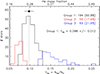 |
Fig. 1. He abundance distributions for the three groups of stars introduced in Sect. 4.1. The vertical dotted line indicates the present-day cosmic reference value provided by Nieva & Przybilla (2012). The black dot and horizontal line indicate the mean and standard deviation associated with Group 1 stars. |
4.2. Comparison with results from the literature
Figure 2 shows a comparison of our He abundance estimates with some others available in the literature. We focus on four recent studies selected because they provide abundances for at least ten stars in common with our sample: namely Repolust et al. (2004), Martins et al. (2015b), Markova et al. (2018) and Aschenbrenner et al. (2023). The first two are based on the FASTWIND atmosphere code, as in our study; the third employs CMFGEN (Hillier & Miller 1998); and the last one relies on a hybrid analysis combining ATLAS9 atmosphere models (Kurucz 1993) with spectral synthesis calculations performed with DETAIL and SURFACE (see also Nieva & Przybilla 2012).
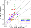 |
Fig. 2. Comparison of He abundances for a sample of 67 stars in common with the literature and 48 stars independently analysed for this work using the code MAUI. The open symbols refer to stars for which we have provided a Q2 or Q3 quality flag to the FASTWIND fits (see Tables D.1 to D.3). The 1-to-1 relation and 25% tolerance region are shown as dashed and dotted lines, respectively. The cross in the top left corner indicates the typical uncertainties in the YHe estimates. |
Taking into account the associated uncertainties, we find a reasonably good agreement for most of the (67) stars in common with any of the abovementioned studies. Nevertheless, a small subset of (14) stars shows discrepancies beyond 25%. Appendix B provides additional notes on these specific stars.
We also performed a fully independent analysis of a subsample of ∼50 of the stars under study with the code MAUI (Urbaneja 2026). MAUI is a modular framework that builds on a statistical emulator (in this case of FASTWIND synthetic spectra) with supervised machine-learning techniques and, coupled with MCMC sampling, enables a robust and efficient spectroscopic inference for massive star parameters and surface abundances. In particular, this subsample of stars has been specifically selected to cover the full range of Teff, log g, YHe, and v sin i characterising the complete sample analysed with IACOB-GBAT. As illustrated in Fig. 2, the agreement of results between these two analysis approaches is also quite remarkable.
4.3. The Hunter and spectroscopic HR diagrams
Figure 3 shows the distribution of stars in a modified version of the Hunter diagram (c.f. Hunter et al. 2008), where the He abundance is used instead of nitrogen. Stars classified as ON or identified as SB1 and/or RWs are highlighted separately. For reference, we indicate in grey the main range of He abundances (mean value ±2 σ) covered by stars in Group 1, and with grey dashed lines the step values in YHe defining the grid of FASTWIND models incorporated into IACOB-GBAT. We also report the percentage of He-rich stars among the samples with a v sin i below and above 200 km s−1, respectively. This threshold has been adopted in several previous studies to separate the main low v sin i component from the high-velocity tail in the distribution of projected rotational velocities commonly found in O stars (e.g. de Mink et al. 2013; Ramírez-Agudelo et al. 2013; Holgado et al. 2022; Sana et al. 2022; Britavskiy et al. 2023; Carretero-Castrillo et al. 2026). As proposed by de Mink et al. (2013), stars with v sin i exceeding this threshold are most likely the products of binary interaction – following mass-transfer or merger events – rather than massive stars formed in isolation with such rapid rotation.
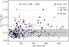 |
Fig. 3. Distribution of the 318 Galactic O-type stars in a modified Hunter diagram, using He abundance instead of nitrogen on the y-axis. The fractions of He-rich stars in the slow- and fast-rotating subsamples are indicated, assuming v sin i = 200 km s−1 as the dividing threshold. ON, SB1, and RW stars are indicated with red small circles, blue crosses, and grey circles, respectively. |
Figure 4 presents the location of the stars in the three He abundance groups defined in Sect. 4.1 within a spectroscopic Hertzsprung–Russell diagram (sHRD; Langer & Kudritzki 2014). As in Fig. 4, ON, SB1 and RW stars are differentiated from the rest of the sample. For reference, we also show the position of the ZAMS and the evolutionary tracks computed with the GENEC code for an initial spin rate vini/vcrit = 0.4 (Ekström et al. 2012). Sections of the tracks where the surface He abundance is larger than 1.3 times the initial abundance are highlighted with dashed green lines. In this case, the predicted increase of the He abundance at the stellar surface is driven by the internal transport processes implemented in the models, together with the progressive removal of the outer stellar layers by winds for stars above ∼30 M⊙. Although we used these single star evolution tracks as reference to show a extreme case of surface enrichment due to rotational mixing (see further notes in Sect. 5.2), we note that the initial spin rate considered in these models is definitely too high when accounting from the results presented in Holgado et al. (2022). These authors proposed that the peak of the spin distribution at birth for O-type stars is most likely located at vini/vcrit = 0.10 – 0.15.
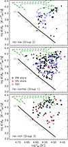 |
Fig. 4. Distribution of our sample of 318 Galactic O-type stars in a sHRD separated by the three He abundance groups described in Sect. 4.1. Evolutionary tracks from Ekström et al. (2012) for an initial spin rate vini/vcrit = 0.4 are depicted for reference purposes, highlighting in green the sections of the tracks where the He surface abundance reaches over 1.3 times the initial abundance. The symbols are the same as in Fig. 3. |
4.4. Statistical properties of the runaway and SB1 samples
As stated in Sect. 2, we have runaway classifications for 268 stars (84.3%) in our working sample of 318 objects. We also have sufficient multi-epoch spectroscopy4 to assess the SB1 status for 237 stars (74.5%). In combination with their locations in the Hunter and sHR diagrams (Figs. 3 and 4, respectively), we summarize the corresponding runaway and SB1 statistics for the full sample, as well as for subsamples defined by He abundance and v sin i, in columns 2–4 and 5–7 of Table 3, respectively.
Complementing this information, we also find that He-rich stars are much more common among runaways: 39% of the RW sample (comprising 77 stars) are He-rich, compared to only 17% in the non-RW sample (191 stars). Additionally, He-rich stars are less common among SB1 systems: they represent 14% of the 73 SB1 sample, compared to 28% among the 164 LS sample. In this regard, we remind that a certain percentage of stars identified as LS could be merger products, disrupted binaries, or undetected SB1 systems (due to the still insufficient number of available epochs, or the difficulty to separate the effect of intrinsic variability from the orbital motion in a binary system where the amplitude of radial velocity variation is below 15–20 km s−1; Simón-Díaz et al. 2024).
5. Discussion
5.1. The He-low sample
One of the first aspects that drew our attention was the non-negligible fraction of stars (∼18%) for which the default IACOB-GBAT analysis yielded He abundances in the range YHe = 0.06–0.08 (see Fig. 1). These values reach well below the lower limits of He abundances typically reported for Galactic early B-type stars (e.g. Lyubimkov 1975; Nieva & Przybilla 2012), our Sun (e.g. Serenelli & Basu 2010; Moharana et al. 2024), blue compact very metal-poor dwarf galaxies (e.g. Izotov et al. 1999), and interstellar medium estimates based on radio recombination line observations (e.g. Tsivilev & Krasnov 2023). Such determinations have often been regarded as representative of the primordial He abundance (Pagel 2000).
Given this context, it is natural to suspect that our low He abundance determinations are not physically meaningful, but rather result from limitations in the analysis. Potential contributors include incorrect estimates of microturbulence or wind properties, modelling issues in certain regions of parameter space (e.g. Teff or log g), and contamination from faint, unresolved companions whose continuum contribution can dilute the diagnostic He lines. To investigate these possibilities, we compared stars in Groups 2 (He-low) and 1 (He-normal) in terms of their location in the sHRD (Fig. 4) and their microturbulent velocities, as derived from the default IACOB-GBAT analysis. We also examined whether SB1 systems are overrepresented among He-low stars (Table 3).
These comparisons reveal no significant differences in ξt between the two groups. In particular, the fraction of He-low stars actually decreases with increasing microturbulence, which is the opposite of what would be expected if their abundances were being systematically underestimated due to overestimated ξt. Likewise, although Group 2 stars appear to cluster in a specific region of the sHRD (top panel in Fig. 4), that region also contains stars with normal He abundances, making systematic modelling limitations an unlikely explanation. Moreover, the relative percentages of He-low stars are similar among targets with assigned quality flags Q1, Q2, and Q3 (Table D.1), again suggesting that modelling issues are not the primary cause of the anomalously low He abundances.
Altogether, these results leave as the most plausible explanation that many of the He-low stars are systems with undetected companions, for which the IACOB-GBAT analysis yields spuriously low abundances. Interestingly the fraction of SB1 systems is larger in the He-low group (44%) than in the He-normal one (33%). Also, formal tests based on synthetic spectra computed with FASTWIND – in which the diagnostic lines were diluted by only 10% – show that a similar IACOB-GBAT analysis to that performed here can easily underestimate the He abundance by 0.01–0.02 (Martínez-Sebastián et al., subm.). These tests therefore support the hypothesis that undetected companions (possibly combined with minor modelling effects) are responsible for the low He abundances found in Group 2 stars.
5.2. The He-rich sample in the context of single star evolution
As illustrated in Fig. 1, the distribution of surface He abundances is characterized by: (1) a dominant component comprising ∼80% of the sample (Groups 1 and 2), centered at YHe ≈ 0.095 and displaying a dispersion broadly consistent with the He abundance uncertainties of our analysis, and (2) an extended tail of He-enriched stars (Group 3), accounting for ∼20% of the sample, with abundances covering the range YHe ∼ 0.12 – 0.25.
Rotationally induced mixing has been considered for more than three decades as the most likely explanation for the occurrence of these He-rich stars, with the efficiency of this process predicted to increase with both initial mass and rotation rate. (e.g. Maeder & Meynet 2000; Heger & Langer 2000; Meynet & Maeder 2000; Brott et al. 2011; Ekström et al. 2012). However, we provide below two independent pieces of evidence indicating that this internal mixing mechanism alone cannot explain the observed distribution of stars under study in the He – v sin i and sHR diagrams presented in Figs. 3 and 4, respectively.
As in previous studies focusing on nitrogen (e.g. Hunter et al. 2008; Rivero González et al. 2012; Bouret et al. 2013; Grin et al. 2017), the He – v sin i diagram does not reveal a clear correlation between the two quantities. Furthermore, there is a non-negligible number of He-rich stars with relatively low v sin i. In addition, while the percentage of He-rich stars within the tail of fast-rotators is larger than in the main low v sin i component (32% vs 19%; see Fig. 3), there is still a dominance of He-normal stars among the stars with v sin i > 200 km s−1.
This long-standing issue has been extensively discussed in the literature (Brott et al. 2011; Maeder et al. 2014; Martins et al. 2017), where several effects have been proposed to partially account for the observed scatter when examining individual stars. For example, age may explain the presence of some fast-rotating stars among the He-normal group, as they may simply be too young to display detectable abundance changes. This is evident from the evolutionary tracks shown in Fig. 4 where, even for stars born spinning at 40% of their critical velocity, only at the very end of the main-sequence the He produced in the core is reaching the stellar surface to a detectable level. Similarly, the group of He-rich stars with low v sin i could in principle be rapid rotators observed pole-on; however, this is unlikely given the large number of stars with these characteristics.
Focusing only on the He – v sin i diagram presented in Fig. 3, another plausible scenario might be that these He-rich, low v sin i objects provide observational evidence for efficient surface-braking mechanisms operating during the main-sequence phase, reducing the surface rotation rate while internal mixing continues to transport nuclear-processed material to the surface (see e.g. Ekström et al. 2012). However, this proposal would be in tension with the observational findings by Holgado et al. (2022), de Burgos et al. (2024), and Nathaniel et al. (2025) about the non-detection of a clear surface braking of massive stars along their main-sequence evolution.
A more critical challenge to the rotational-mixing scenario arises from the distribution of He-rich stars in the sHRD. A substantial fraction of Group 3 stars (∼47%, i.e. those located below log (ℒ/ℒ⊙) ∼ 4.0) occupy regions of the diagram where the rotating GENEC tracks of Ekström et al. (2012) do not predict such levels of enrichment. This is illustrated in the bottom panel of Fig. 4, where the segments of the evolutionary tracks having He abundances > 1.3 times higher than the initial value (comparable with Group 3 stars) are marked with thick dashed green lines. Even these models – among the most efficient in producing surface enrichment (see Keszthelyi et al. 2022) – fail to reproduce the observed population. This tension is also further strengthened by the fact that most O-type stars are likely born with initial equatorial velocities below 0.2 vcrit (Holgado et al. 2022), making very rapid initial rotation an unlikely explanation for the He-rich stars.
These results provide strong evidence that rotational mixing alone cannot be the dominant driver of surface He enrichment in Galactic O-type stars. Instead, our findings reinforce the growing consensus that additional mechanisms – most notably binary interaction, as shown in next sections – might play a central role in shaping the observed He-abundance distribution.
5.3. Some insights from binary evolution
A large percentage of massive O stars are commonly found to be part of binary or higher-order systems (e.g. Kobulnicky & Fryer 2007; Kobulnicky et al. 2014; Chini et al. 2012; Sana et al. 2013; Moe & Di Stefano 2017; Sana et al. 2025; Mahy et al. 2009, 2013; Barbá et al. 2017; Offner et al. 2023; Barbá et al. 2026). Sana et al. (2012) indicated that more than 70% of all massive stars will exchange mass with a companion at some point in their lives, leading to a binary merger in one-third of the cases. These relatively recent findings have revived a long-standing concern in stellar astrophysics – namely, the importance of accounting for binary evolution when interpreting the observed properties of massive-star populations (see e.g. reviews by Vanbeveren 1988, 1993, 2004; Vanbeveren & Mennekens 2017; Marchant & Bodensteiner 2024; Marchant 2026, and references therein).
Mass transfer and merger events can modify the spin rates and surface chemical composition of the stars involved in the interaction (e.g. de Mink et al. 2013; Farmer et al. 2023; Menon et al. 2024; Jin et al. 2026). Moreover, binary-interaction products will often be observed as apparently single stars (de Mink et al. 2014). This will certainly be the case for merger remnants as well as runaway stars resulting from disrupted binaries following the supernova explosion of the initially more massive companion, but also for binary systems in which the post–mass-transfer donor becomes difficult to detect, either directly in the optical spectrum or through radial velocity variations of the currently more massive and optically more luminous component, the mass gainer. Only under specific orbital configurations and mass ratios will these systems be detected as SB1.
Although a detailed comparison between our observational results and theoretical predictions for binary-interaction products lies beyond the scope of this work, we briefly comment on the expected behavior of mass gainers from binary evolution models. Figure 5 depicts the distribution in the sHRD of a sample of mass gainers as predicted by computations performed by Jin et al. (2026). These authors have created a comprehensive grid of massive binary evolution models for solar metallicity computed with the MESA stellar evolution code (first introduced in Paxton et al. 2011). They covered a range of initial primary star masses from 5 to 100 M⊙. Their computations incorporate detailed stellar and binary physics, including internal differential rotation, magnetic angular momentum transport, mass-dependent overshooting, stellar wind mass-loss, mass and angular momentum transfer and tidal interaction. Specifically, the outcome of their computations presented in Fig. 5 corresponds to the moment just after mass accretion and thermal relaxation has occurred, and before further nuclear-timescale evolution has taken place.
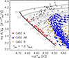 |
Fig. 5. Distribution in the sHRD of the birth location of mass gainers as predicted by the binary evolution computations by Jin et al. (2026). The full sample of gainers are depicted in grey, while those with enriched He abundances are highlighted with colours separating the mass-transfer cases A (red), B (orange), and AB (blue). Single star evolutionary tracks computed with the MESA stellar evolution code by Jin et al. (2024a) and used as the basis for the binary evolution computation are also depicted for reference purposes. The open circles show the location of the He-rich group of O-type stars from our study. |
Within the full sample of resulting mass gainers, we highlight those with surface He abundances exceeding 1.2 times the initial value. This subsample is expected to correspond to the stars comprising Group 3, whose locations are shown again in Fig. 5 with open circles for reference. We recall that the positions of the highlighted gainers should be interpreted as their effective “birth” locations following the mass-transfer event. From these positions, all of these stars are expected to continue their subsequent evolution toward lower effective temperatures.
From inspection of Fig. 5, and bearing in mind that He-contaminated mass gainers are expected to remain He-rich throughout their subsequent evolution (Jin et al. 2026), we can draw a general conclusion. Binary interaction through mass-transfer events can account for the presence of He-rich O-type stars in regions of the sHRD where rotating single-star evolutionary models fail to reproduce the observations (bottom panel of Fig. 4). In particular, the computations performed by Jin et al. (2026) indicate that strongly He-enriched case A mass gainers (red filled circles) can reach the single-star ZAMS line before continuing their post mass-transfer evolution. These objects correspond to secondary stars from the highest-mass binaries in the model grid, which only undergo fast case A mass transfer (see Sect. 3.1.2 in Jin et al. 2026). In addition, He-rich gainers resulting from case B (orange) and AB (blue) mass-transfer can also populate the region of the sHRD under study. There is a gap between the ZAMS and their positions in the diagram because the secondaries are already significantly evolved by the time the primaries deplete core hydrogen and case AB or case B mass transfer occurs. However, if mass accretion was larger than assumed in the models computed by Jin et al. (2026), rejuvenation of this second set of gainers might be stronger and hence their birth location would be shifted towards the ZAMS line.
A second conclusion that can be extracted from inspection of Fig. 5 is that binary mass transfer does not operate efficiently at spectroscopic luminosities above log (ℒ/ℒ⊙) ∼ 4.0. This is because also the binary components, in particular the more massive potential donor star, partly self-strip their envelope by winds, such that much less mass is transferred if Roche- lobe overflow (RLOF) occurs. At the same time, this wind stripping keeps the binary components more compact, such that RLOF is often avoided all together (see also Pauli et al. 2022). Therefore, the binary models do produce many He-enriched primary and secondary stars, in a region similar to that where He enrichment is indicated for the single star models in Fig. 4, but they do not appear in Fig. 5 as it shows only He-rich post mass transfer mass gainer models. Furthermore, additional evolutionary pathways not represented in Fig. 5 may also contribute. For instance, in reverse Algol systems (Sen et al. 2023), the donor star can remain the more luminous component of the binary, exhibit surface He enrichment, and populate the upper part of the sHRD. In addition, mass accretion efficiency is one of the most uncertain parameters in binary evolution, and a more efficient mass accretion than adopted in the models of Jin et al. (2026) can help populate the upper sHRD with He-enriched mass gainers. Complementarily, although not explored here, merger events are also a viable explanation for some of the identified He-rich stars (Menon et al. 2024).
Also remarkable is the fraction of stars with He-enriched surfaces that show a clear dependence on (spectroscopic) luminosity. Below log (ℒ/ℒ⊙) ∼ 4.0 – where neither rotational mixing nor wind stripping is expected to operate efficiently to enrich the surface with He – the percentage of He-rich stars amounts to ∼16%. This percentage increases to ∼31% at higher luminosities, where self-stripping by winds and rotational mixing becomes more effective in both single and binary stars.
5.4. The YHe – v sin i diagram
The binary-evolution channel also introduces key elements for interpreting the distribution of O-type stars in the YHe – v sin i diagram (Fig. 3), particularly in light of the shortcomings of the single star scenario (Sect. 5.2).
In systems undergoing case A mass transfer, the observed surface rotation of the He-rich gainer is not expected to exceed ∼200–250 km s−1, because tidal forces efficiently counteract the spin-up induced by mass accretion (e.g. de Mink et al. 2013; Langer et al. 2020, and references therein). This could explain the non-negligible fraction of He-rich stars with v sin i < 200 km s−1 (see Fig. 3 and Table 3). The same tidal effects may also explain for the relative scarcity of He-rich stars with v sin i ≲ 50 km s−1). Additional channels – such as reverse-Algol systems, luminous wind-stripped single and binary stars, and stellar mergers – may also contribute to this population.
In case B (or AB) mass-transfer events, tidal forces are no longer sufficiently strong to prevent substantial spin-up of the gainer. Such interactions can therefore produce stars that simultaneously exhibit rapid rotation and – as shown in Sect. 5.3 – enhanced surface He abundances. Rotational mixing may also contribute to this population to some extent.
Finally, Jin et al. (2026) predicts that not all mass-transfer events lead to He-rich gainers. In addition, some pre-interaction binaries with low mass ratios may contribute to the He-normal population – in many cases, but not always, detected as SB1 systems – alongside stars evolving effectively as single.
Taken together, these effects can account for the coexistence of He-rich and He-normal stars across a wide range of projected rotational velocities and binary classifications, as observed in our sample.
5.5. Further insights from the RWs and SB1 systems
Runaway stars provide valuable clues to identify past binary interactions. The peculiar velocities are generally attributed to either the binary supernova scenario (BSS; Blaauw 1961) or to the dynamical ejection scenario (DES; Poveda et al. 1967). Among these channels, the BSS is particularly relevant for understanding the surface chemical properties of massive stars. Prior to the supernova (SN), mass transfer in the binary can spin up the future RW (the gainer) and modify its chemical composition, potentially leading to He enrichment (Packet 1981; van den Heuvel 1985; Blaauw 1993). After the SN, the former binary will most likely result unbound, although not necessarily (e.g. Renzo et al. 2019; Carretero-Castrillo et al. 2026). These signatures – fast rotation, altered chemical abundances, and absence of detectable companions – are therefore expected in RW stars produced via binary interaction.
In Sect. 4.4, we showed that runaways are significantly more frequent among He-rich stars (48%) than among He-normal ones (24%), with the fraction increasing to 62% when considering only fast rotators. This result provides strong additional support for the binary-interaction scenario as the primary explanation for the presence of He-enriched surfaces among O-type stars, and extends the conclusions reached by Britavskiy et al. (2023) and Carretero-Castrillo et al. (2026) regarding the impact of binary interaction in these type of stars.
Conversely, the fraction of detected SB1 systems is lower in the He-rich sample (18%) compared to the He-normal population (33%). Several effects can account for this reduced SB1 incidence. As discussed above, a large fraction of He-rich stars are identified as runaways, suggesting that they are mass gainers in systems that underwent mass transfer – leading to He enrichment – followed by disruption after the supernova explosion of the donor star (see Sect. 5.3). Consistent with this picture, only four out of the 30 He-rich runaway stars in our sample are detected as SB1 systems (Fig. 4).
In addition, a small fraction of He-rich stars may be merger products, in which any dynamical signature of binarity has been erased. Finally, some objects may correspond to post–mass-transfer systems that remain bound, but in which the initially more massive star has evolved into a low-mass stripped star or a compact object. In such cases, the donor becomes difficult to detect in the optical spectrum, while the mass gainer – the currently more massive and optically more luminous component – exhibits a relatively small orbital velocity amplitude, making SB1 detection particularly challenging. In this regard, the relatively low incidence of He-enrichment in the SB1s is consistent with the idea that binaries with significant radial velocity variations are mostly pre-interaction systems (de Mink et al. 2014).
5.6. The ON star sample
From basic stellar structure physics and single-star evolution, if the observed surface abundance pattern of H-burning CNO-cycle products in (main-sequence) O-type stars were solely the result of internal mixing, He-rich stars should also display a remarkable enhancement of nitrogen at their surfaces (see e.g. Fig. 1 in Martínez-Sebastián et al. 2025). In this work, the ON qualifier used in spectral classification (Walborn 1970, 1971, 1976; Sota et al. 2011) can serve as a reliable proxy of such a strong N enrichment. These class of O-type stars were first identified by Walborn (1970) as having the N lines in their optical spectra too strong for their spectral types, an anomaly which was postulated to be caused by abundance effects. This hypothesis was later confirmed by specific quantitative spectroscopic analyses (e.g. Schonberner et al. 1988; Martins et al. 2015b).
As noted in Sect. 2, our sample includes 19 ON stars, all of them highlighted in Figs. 3 and 4. While ON stars are not separated from the rest of the population in terms of v sin i (Fig. 3), they show a strong tendency to be found among stars with surfaces enriched in He. This confirms earlier findings by Martins et al. (2015b) based on a smaller dataset.
However, the majority of He-rich stars (∼80%) are not identified as ON. Once more, a piece of observational evidence that seems to indicate that rotationally induced mixing might not be the dominant source of contamination of the stellar surfaces in a non-negligible fraction of O-type stars. We refer to Martínez-Sebastián et al. (2025, 2026) for a more detailed investigation of this result incorporating information about N abundances in a subsample of the stars considered for this work.
6. Conclusions and future prospects
In this work we present strong observational evidence supporting the hypothesis that a large fraction of Galactic O-type stars – classified as apparently single or SB1 systems and presenting surfaces enriched in helium – are products of binary interaction.
Our conclusions are grounded in the first comprehensive and homogeneous quantitative spectroscopic analysis of He abundances in a statistically significant sample of Galactic O-type stars More than half of the stars identified as He-rich occupy regions of the sHRD that are incompatible with the predictions of rotating single-star evolutionary models (even under the most efficient internal mixing assumptions; Ekström et al. 2012). By contrast, these locations can be explained if these objects are mass gainers that have experienced a previous mass-transfer episode (or, in some cases, are the products of stellar mergers).
Binary-evolution models by Jin et al. (2026) predict that mass gainers resulting from case A, B, or AB mass-transfer events can reproduce the properties of the He-rich population found along the main-sequence band spanned by typical single O-type stars (∼15–60 M⊙; see Fig. 5). Although not explored in detail here, some He-rich stars may also be reverse-Algol systems and merger products.
Additional observational clues reinforce this binary-interaction interpretation. The fraction of runaways is roughly a factor of two higher among He-rich stars compared to He-normal ones, while the fraction of detected SB1 systems is somewhat lower. Both trends qualitatively agree with expectations from binary evolution, where mass gainers may become runaways following a supernova explosion, or may lose their binary signature through mergers, unbound binaries, or through the presence of optically faint stripped companions (Blaauw 1961; de Mink et al. 2014).
Surface He abundances hence emerge as an efficient diagnostic to identify potential binary-interaction products, providing an accessible starting point for targeted follow-up observations. More broadly, the combination of Teff, log g, v sin i, and He abundance measurements in statistically meaningful samples of O-type stars already offers valuable constraints for models of binary evolution and population synthesis. These constraints will become even more powerful when complemented with information on other chemical species (C, N, O), binary and runaway status, orbital parameters of SB1 systems (e.g. periods and radial velocity amplitudes; Barbá et al. 2026), and accurate stellar masses and luminosities (Holgado et al. 2025). The combination of all this observational information will also help to constrain to what extent the He-rich stars located above log (ℒ/ℒ⊙) ∼ 4.0 are also the result of binary interaction, they are produced by a combination of rotationally induced mixing and wind-stripping, or there is combination of various of these effects.
From 318 Galactic O-type stars gathered by the IACOB project, we identified approximately 70 with clear He enrichment, corresponding to ∼22% of the sample. Among them, 11 are SB1 systems whose orbital properties warrant dedicated multiwavelenght follow-up. In this sense, our study represents an intermediate step between earlier analyses of Galactic O-type stars – typically limited to a few dozen objects – and the order-of-magnitude increase in sample size that will soon be enabled by upcoming large-scale spectroscopic surveys such as WEAVE (Jin et al. 2024b) and 4MOST (de Jong et al. 2019).
Finally, while this paper has focused primarily on helium, Martínez-Sebastián et al. (2025, 2026) presents a complementary work investigating N abundances for a subset of these stars (those with v sin i ≲ 150 km s−1). Together, these studies pave the way for a new generation of observational constraints on massive-star evolution in both single and binary channels.
Data availability
Tables D.1, D.2, and D.3 are available at the CDS via https://cdsarc.cds.unistra.fr/viz-bin/cat/J/A+A/711/A151.
Acknowledgments
S.S-D., G.H., C.M-S. and A.H. acknowledge support from the State Research Agency (AEI) of the Spanish Ministry of Science and Innovation (MICIN) and the European Regional Development Fund, FEDER under grants PID2021-122397NB-C21 and PID2024-159329NB-C21. This project received the support from the “La Caixa” Foundation (ID 100010434) under the fellowship code LCF/BQ/PI23/11970035. MC-C, JMP, and MR acknowledge financial support from the State Agency for Research of the Spanish Ministry of Science and Innovation under grants PID2022-136828NB-C41/AEI/10.13039/501100011033/ERDF/EU, and PID2022-138172NB-C43/AEI/10.13039/501100011033/ERDF/EU, and through the Unit of Excellence María de Maeztu 2025-2029 award to the Institute of Cosmos Sciences (CEX2024-001451-M, MICIU/AEI/10.13039/501100011033). The project leading to this application has received funding from European Commission (EC) under Project OCEANS – Overcoming challenges in the evolution and nature of massive stars, HORIZON-MSCA-2023-SE-01, No G.A 101183150 Funded by the European Union. This work has made use of data from the European Space Agency (ESA) mission Gaia (https://www.cosmos.esa.int/Gaia), processed by the Gaia Data Processing and Analysis Consortium (DPAC, https://www.cosmos.esa.int/web/Gaia/dpac/consortium). Funding for the DPAC has been provided by national institutions, in particular the institutions participating in the Gaia Multilateral Agreement. Based on observations made with the Nordic Optical Telescope, operated by NOTSA, and the Mercator Telescope, operated by the Flemish Community, both at the Observatorio del Roque de los Muchachos (La Palma, Spain) of the Instituto de Astrofísica de Canarias. Based on observations at the European Southern Observatory in programs 073.D-0609(A), 077.B-0348(A), 079.D-0564(A), 079.D-0564(C), 081.D-2008(A), 081.D-2008(B), 083.D-0589(A), 083.D-0589(B), 086.D-0997(A), 086.D-0997(B), 087.D-0946(A), 089.D-0975(A).
References
- Aerts, C., Molenberghs, G., Kenward, M. G., & Neiner, C. 2014, ApJ, 781, 88 [Google Scholar]
- Aschenbrenner, P., Przybilla, N., & Butler, K. 2023, A&A, 671, A36 [NASA ADS] [CrossRef] [EDP Sciences] [Google Scholar]
- Barbá, R. H., Gamen, R., Arias, J. I., et al. 2010, Rev. Mex. Astron. Astrofis. Conf. Ser., 38, 30 [Google Scholar]
- Barbá, R. H., Gamen, R., Arias, J. I., & Morrell, N. I. 2017, IAU Symp., 329, 89 [Google Scholar]
- Barbá, R. H., Gamen, R., Morrell, N. I., et al. 2026, A&A, 708, A98 [NASA ADS] [CrossRef] [EDP Sciences] [Google Scholar]
- Blaauw, A. 1961, Bull. Astron. Inst. Netherlands, 15, 265 [NASA ADS] [Google Scholar]
- Blaauw, A. 1993, ASP Conf. Ser., 35, 207 [Google Scholar]
- Bohannan, B., Abbott, D. C., Voels, S. A., & Hummer, D. G. 1986, ApJ, 308, 728 [Google Scholar]
- Bouret, J. C., Hillier, D. J., Lanz, T., & Fullerton, A. W. 2012, A&A, 544, A67 [NASA ADS] [CrossRef] [EDP Sciences] [Google Scholar]
- Bouret, J. C., Lanz, T., Martins, F., et al. 2013, A&A, 555, A1 [NASA ADS] [CrossRef] [EDP Sciences] [Google Scholar]
- Bouret, J. C., Martins, F., Hillier, D. J., et al. 2021, A&A, 647, A134 [NASA ADS] [CrossRef] [EDP Sciences] [Google Scholar]
- Brinkman, H. E., Tkachenko, A., & Aerts, C. 2025, A&A, 702, A119 [NASA ADS] [CrossRef] [EDP Sciences] [Google Scholar]
- Britavskiy, N., Simón-Díaz, S., Holgado, G., et al. 2023, A&A, 672, A22 [NASA ADS] [CrossRef] [EDP Sciences] [Google Scholar]
- Brott, I., de Mink, S. E., Cantiello, M., et al. 2011, A&A, 530, A115 [NASA ADS] [CrossRef] [EDP Sciences] [Google Scholar]
- Burssens, S., Simón-Díaz, S., Bowman, D. M., et al. 2020, A&A, 639, A81 [NASA ADS] [CrossRef] [EDP Sciences] [Google Scholar]
- Carretero-Castrillo, M., Ribó, M., & Paredes, J. M. 2023, A&A, 679, A109 [NASA ADS] [CrossRef] [EDP Sciences] [Google Scholar]
- Carretero-Castrillo, M., Ribó, M., Paredes, J. M., et al. 2026, A&A, 705, A215 [NASA ADS] [CrossRef] [EDP Sciences] [Google Scholar]
- Cazorla, C., Nazé, Y., Morel, T., et al. 2017, A&A, 604, A123 [NASA ADS] [CrossRef] [EDP Sciences] [Google Scholar]
- Chini, R., Hoffmeister, V. H., Nasseri, A., Stahl, O., & Zinnecker, H. 2012, MNRAS, 424, 1925 [Google Scholar]
- de Burgos, A., Simón-Díaz, S., Urbaneja, M. A., & Puls, J. 2024, A&A, 687, A228 [NASA ADS] [CrossRef] [EDP Sciences] [Google Scholar]
- de Jong, R. S., Agertz, O., Berbel, A. A., et al. 2019, The Messenger, 175, 3 [NASA ADS] [Google Scholar]
- de Mink, S. E., Cantiello, M., Langer, N., et al. 2009, A&A, 497, 243 [NASA ADS] [CrossRef] [EDP Sciences] [Google Scholar]
- de Mink, S. E., Langer, N., Izzard, R. G., Sana, H., & de Koter, A. 2013, ApJ, 764, 166 [Google Scholar]
- de Mink, S. E., Sana, H., Langer, N., Izzard, R. G., & Schneider, F. R. N. 2014, ApJ, 782, 7 [Google Scholar]
- Dufton, P. L., Thompson, A., Crowther, P. A., et al. 2018, A&A, 615, A101 [NASA ADS] [CrossRef] [EDP Sciences] [Google Scholar]
- Dufton, P. L., Evans, C. J., Lennon, D. J., & Hunter, I. 2020, A&A, 634, A6 [NASA ADS] [CrossRef] [EDP Sciences] [Google Scholar]
- Ekström, S., Georgy, C., Eggenberger, P., et al. 2012, A&A, 537, A146 [Google Scholar]
- Farmer, R., Laplace, E., Ma, J.-Z., de Mink, S. E., & Justham, S. 2023, ApJ, 948, 111 [NASA ADS] [CrossRef] [Google Scholar]
- Frischknecht, U., Hirschi, R., Meynet, G., et al. 2010, A&A, 522, A39 [NASA ADS] [CrossRef] [EDP Sciences] [Google Scholar]
- Gaia Collaboration (Brown, A. G. A., et al.) 2016, A&A, 595, A2 [NASA ADS] [CrossRef] [EDP Sciences] [Google Scholar]
- Gaia Collaboration (Vallenari, A., et al.) 2023, A&A, 674, A1 [NASA ADS] [CrossRef] [EDP Sciences] [Google Scholar]
- Gies, D. R., Mason, B. D., Bagnuolo, W. G., Jr, et al. 1997, ApJ, 475, L49 [NASA ADS] [CrossRef] [Google Scholar]
- Maíz Apellániz, J., Alonso Moragón, A., de Zárate, Ortiz, Alcarazo, L., & GOSSS Team 2017, in Highlights on Spanish Astrophysics IX, eds. S. Arribas, A. Alonso-Herrero, F. Figueras, et al., 509 [Google Scholar]
- Grin, N. J., Ramírez-Agudelo, O. H., de Koter, A., et al. 2017, A&A, 600, A82 [NASA ADS] [CrossRef] [EDP Sciences] [Google Scholar]
- Groenewegen, M. A. T., Lamers, H. J. G. L. M., & Pauldrach, A. W. A. 1989, A&A, 221, 78 [NASA ADS] [Google Scholar]
- Heger, A., & Langer, N. 2000, ApJ, 544, 1016 [CrossRef] [Google Scholar]
- Herrero, A., Kudritzki, R. P., Vilchez, J. M., et al. 1992, A&A, 261, 209 [NASA ADS] [Google Scholar]
- Herrero, A., Corral, L. J., Villamariz, M. R., & Martín, E. L. 1999, A&A, 348, 542 [NASA ADS] [Google Scholar]
- Herrero, A., Puls, J., & Villamariz, M. R. 2000, A&A, 354, 193 [NASA ADS] [Google Scholar]
- Hillier, D. J., & Miller, D. L. 1998, ApJ, 496, 407 [NASA ADS] [CrossRef] [Google Scholar]
- Holgado, G. 2019, Ph.D. Thesis, Astrophysical Institute of the Canaries, University of La Laguna, Spain [Google Scholar]
- Holgado, G., Simón-Díaz, S., Barbá, R. H., et al. 2018, A&A, 613, A65 [NASA ADS] [CrossRef] [EDP Sciences] [Google Scholar]
- Holgado, G., Simón-Díaz, S., Haemmerlé, L., et al. 2020, A&A, 638, A157 [NASA ADS] [CrossRef] [EDP Sciences] [Google Scholar]
- Holgado, G., Simón-Díaz, S., Herrero, A., & Barbá, R. H. 2022, A&A, 665, A150 [NASA ADS] [CrossRef] [EDP Sciences] [Google Scholar]
- Holgado, G., Simón-Díaz, S., & Herrero, A. 2025, A&A, 703, A175 [NASA ADS] [CrossRef] [EDP Sciences] [Google Scholar]
- Hunter, I., Brott, I., Lennon, D. J., et al. 2008, ApJ, 676, L29 [NASA ADS] [CrossRef] [Google Scholar]
- Hunter, I., Brott, I., Langer, N., et al. 2009, A&A, 496, 841 [NASA ADS] [CrossRef] [EDP Sciences] [Google Scholar]
- Simón-Díaz, S., Pérez Prieto, J. A., Holgado, G., de Burgos, A., & Iacob Team 2020, in XIV.0 Scientific Meeting (virtual) of the Spanish Astronomical Society, 187 [Google Scholar]
- Izotov, Y. I., Chaffee, F. H., Foltz, C. B., et al. 1999, ApJ, 527, 757 [NASA ADS] [CrossRef] [Google Scholar]
- Jin, H., Langer, N., Lennon, D. J., & Proffitt, C. R. 2024a, A&A, 690, A135 [NASA ADS] [CrossRef] [EDP Sciences] [Google Scholar]
- Jin, S., Trager, S. C., Dalton, G. B., et al. 2024b, MNRAS, 530, 2688 [NASA ADS] [CrossRef] [Google Scholar]
- Jin, H., Langer, N., Ercolino, A., & de Mink, S. E. 2026, A&A, 707, A56 [NASA ADS] [CrossRef] [EDP Sciences] [Google Scholar]
- Keszthelyi, Z., Meynet, G., Georgy, C., et al. 2019, MNRAS, 485, 5843 [NASA ADS] [CrossRef] [Google Scholar]
- Keszthelyi, Z., Meynet, G., Shultz, M. E., et al. 2020, MNRAS, 493, 518 [NASA ADS] [CrossRef] [Google Scholar]
- Keszthelyi, Z., de Koter, A., Götberg, Y., et al. 2022, MNRAS, 517, 2028 [Google Scholar]
- Kobulnicky, H. A., & Fryer, C. L. 2007, ApJ, 670, 747 [NASA ADS] [CrossRef] [Google Scholar]
- Kobulnicky, H. A., Kiminki, D. C., Lundquist, M. J., et al. 2014, ApJS, 213, 34 [Google Scholar]
- Kudritzki, R. P., Simon, K. P., & Hamann, W. R. 1983, A&A, 118, 245 [Google Scholar]
- Kurucz, R. L. 1993, Atomic Line Data, Kurucz CD-ROM No. 2-12 (Cambridge, MA: Smithsonian Astrophysical Observatory) [Google Scholar]
- Langer, N. 1992, A&A, 265, L17 [NASA ADS] [Google Scholar]
- Langer, N., & Kudritzki, R. P. 2014, A&A, 564, A52 [NASA ADS] [CrossRef] [EDP Sciences] [Google Scholar]
- Langer, N., Schürmann, C., Stoll, K., et al. 2020, A&A, 638, A39 [NASA ADS] [CrossRef] [EDP Sciences] [Google Scholar]
- Lyubimkov, A. S. 1975, Astrophysics, 11, 462 [Google Scholar]
- Maeder, A. 1987, A&A, 178, 159 [NASA ADS] [Google Scholar]
- Maeder, A. 1990, A&AS, 84, 139 [NASA ADS] [Google Scholar]
- Maeder, A., & Meynet, G. 2000, ARA&A, 38, 143 [Google Scholar]
- Maeder, A., Przybilla, N., Nieva, M.-F., et al. 2014, A&A, 565, A39 [NASA ADS] [CrossRef] [EDP Sciences] [Google Scholar]
- Mahy, L., Nazé, Y., Rauw, G., et al. 2009, A&A, 502, 937 [NASA ADS] [CrossRef] [EDP Sciences] [Google Scholar]
- Mahy, L., Rauw, G., De Becker, M., Eenens, P., & Flores, C. A. 2013, A&A, 550, A27 [NASA ADS] [CrossRef] [EDP Sciences] [Google Scholar]
- Maíz Apellániz, J., Sota, A., Morrell, N. I., et al. 2013, Massive Stars: From alpha to Omega, 198 [Google Scholar]
- Maíz Apellániz, J., Sota, A., Arias, J. I., et al. 2016, ApJS, 224, 4 [CrossRef] [Google Scholar]
- Maíz Apellániz, J., Pantaleoni González, M., Barbá, R. H., et al. 2018, A&A, 616, A149 [NASA ADS] [CrossRef] [EDP Sciences] [Google Scholar]
- Marchant, P. 2026, Encyclopedia Astrophys., 2, 264 [Google Scholar]
- Marchant, P., & Bodensteiner, J. 2024, ARA&A, 62, 21 [NASA ADS] [CrossRef] [Google Scholar]
- Markova, N., Puls, J., & Langer, N. 2018, A&A, 613, A12 [NASA ADS] [CrossRef] [EDP Sciences] [Google Scholar]
- Martínez-Sebastián, C., Simón-Díaz, S., Jin, H., et al. 2025, A&A, 693, L10 [NASA ADS] [CrossRef] [EDP Sciences] [Google Scholar]
- Martínez-Sebastián, C., Holgado, G., Simón-Díaz, S., Martins, F., & Puls, J. 2026, A&A, 711, A152 [NASA ADS] [CrossRef] [EDP Sciences] [Google Scholar]
- Martins, F., Hervé, A., Bouret, J. C., et al. 2015a, A&A, 575, A34 [NASA ADS] [CrossRef] [EDP Sciences] [Google Scholar]
- Martins, F., Simón-Díaz, S., Palacios, A., et al. 2015b, A&A, 578, A109 [NASA ADS] [CrossRef] [EDP Sciences] [Google Scholar]
- Martins, F., Foschino, S., Bouret, J. C., Barbá, R., & Howarth, I. 2016, A&A, 588, A64 [NASA ADS] [CrossRef] [EDP Sciences] [Google Scholar]
- Martins, F., Simón-Díaz, S., Barbá, R. H., Gamen, R. C., & Ekström, S. 2017, A&A, 599, A30 [NASA ADS] [CrossRef] [EDP Sciences] [Google Scholar]
- Martins, F., Bouret, J. C., Hillier, D. J., et al. 2024, A&A, 689, A31 [NASA ADS] [CrossRef] [EDP Sciences] [Google Scholar]
- Menon, A., Ercolino, A., Urbaneja, M. A., et al. 2024, ApJ, 963, L42 [NASA ADS] [CrossRef] [Google Scholar]
- Meynet, G., & Maeder, A. 2000, A&A, 361, 101 [NASA ADS] [Google Scholar]
- Moe, M., & Di Stefano, R. 2017, ApJS, 230, 15 [Google Scholar]
- Moharana, S., Hema, B. P., & Pandey, G. 2024, ApJ, 974, 312 [Google Scholar]
- Mokiem, M. R., de Koter, A., Puls, J., et al. 2005, A&A, 441, 711 [NASA ADS] [CrossRef] [EDP Sciences] [Google Scholar]
- Mombarg, J. S. G., Varghese, A., & Ratnasingam, R. P. 2025, A&A, 695, A255 [NASA ADS] [CrossRef] [EDP Sciences] [Google Scholar]
- Morel, T., Hubrig, S., & Briquet, M. 2008, A&A, 481, 453 [NASA ADS] [CrossRef] [EDP Sciences] [Google Scholar]
- Najarro, F., Hillier, D. J., Puls, J., Lanz, T., & Martins, F. 2006, A&A, 456, 659 [NASA ADS] [CrossRef] [EDP Sciences] [Google Scholar]
- Nathaniel, K., Langer, N., Simón-Díaz, S., et al. 2025, A&A, 702, A197 [NASA ADS] [CrossRef] [EDP Sciences] [Google Scholar]
- Nieva, M. F., & Przybilla, N. 2012, A&A, 539, A143 [NASA ADS] [CrossRef] [EDP Sciences] [Google Scholar]
- Offner, S. S. R., Moe, M., Kratter, K. M., et al. 2023, ASP Conf. Ser., 534, 275 [NASA ADS] [Google Scholar]
- Packet, W. 1981, A&A, 102, 17 [NASA ADS] [Google Scholar]
- Pagel, B. E. J. 2000, Phys. Rep., 333, 433 [Google Scholar]
- Pauli, D., Langer, N., Aguilera-Dena, D. R., Wang, C., & Marchant, P. 2022, A&A, 667, A58 [NASA ADS] [CrossRef] [EDP Sciences] [Google Scholar]
- Paxton, B., Bildsten, L., Dotter, A., et al. 2011, ApJS, 192, 3 [Google Scholar]
- Poveda, A., Ruiz, J., & Allen, C. 1967, Boletin de los Observatorios Tonantzintla y Tacubaya, 4, 86 [Google Scholar]
- Proffitt, C. R., Lennon, D. J., Langer, N., & Brott, I. 2016, ApJ, 824, 3 [NASA ADS] [CrossRef] [Google Scholar]
- Proffitt, C. R., Jin, H., Daflon, S., et al. 2024, ApJ, 968, 1 [NASA ADS] [CrossRef] [Google Scholar]
- Przybilla, N., Firnstein, M., Nieva, M. F., Meynet, G., & Maeder, A. 2010, A&A, 517, A38 [NASA ADS] [CrossRef] [EDP Sciences] [Google Scholar]
- Puls, J., Kudritzki, R.-P., Herrero, A., et al. 1996, A&A, 305, 171 [NASA ADS] [Google Scholar]
- Puls, J., Urbaneja, M. A., Venero, R., et al. 2005, A&A, 435, 669 [NASA ADS] [CrossRef] [EDP Sciences] [Google Scholar]
- Ramírez-Agudelo, O. H., Simón-Díaz, S., Sana, H., et al. 2013, A&A, 560, A29 [NASA ADS] [CrossRef] [EDP Sciences] [Google Scholar]
- Renzo, M., Zapartas, E., de Mink, S. E., et al. 2019, A&A, 624, A66 [NASA ADS] [CrossRef] [EDP Sciences] [Google Scholar]
- Repolust, T., Puls, J., & Herrero, A. 2004, A&A, 415, 349 [NASA ADS] [CrossRef] [EDP Sciences] [Google Scholar]
- Richards, S. M., Eldridge, J. J., Ghodla, S., & Briel, M. M. 2025, MNRAS, 544, 4146 [Google Scholar]
- Rivero González, J. G., Puls, J., & Najarro, F. 2011, A&A, 536, A58 [NASA ADS] [CrossRef] [EDP Sciences] [Google Scholar]
- Rivero González, J. G., Puls, J., Najarro, F., & Brott, I. 2012, A&A, 537, A79 [NASA ADS] [CrossRef] [EDP Sciences] [Google Scholar]
- Sabín-Sanjulián, C., Simón-Díaz, S., Herrero, A., et al. 2014, A&A, 564, A39 [NASA ADS] [CrossRef] [EDP Sciences] [Google Scholar]
- Sana, H., de Mink, S. E., de Koter, A., et al. 2012, Science, 337, 444 [Google Scholar]
- Sana, H., de Koter, A., de Mink, S. E., et al. 2013, A&A, 550, A107 [NASA ADS] [CrossRef] [EDP Sciences] [Google Scholar]
- Sana, H., Ramírez-Agudelo, O. H., Hénault-Brunet, V., et al. 2022, A&A, 668, L5 [NASA ADS] [CrossRef] [EDP Sciences] [Google Scholar]
- Sana, H., Shenar, T., Bodensteiner, J., et al. 2025, Nat. Astron., 9, 1337 [Google Scholar]
- Santolaya-Rey, A. E., Puls, J., & Herrero, A. 1997, A&A, 323, 488 [NASA ADS] [Google Scholar]
- Schonberner, D., Herrero, A., Becker, S., et al. 1988, A&A, 197, 209 [NASA ADS] [Google Scholar]
- Sen, K., Langer, N., Pauli, D., et al. 2023, A&A, 672, A198 [NASA ADS] [CrossRef] [EDP Sciences] [Google Scholar]
- Serenelli, A. M., & Basu, S. 2010, ApJ, 719, 865 [NASA ADS] [CrossRef] [Google Scholar]
- Simón-Díaz, S., & Herrero, A. 2007, A&A, 468, 1063 [NASA ADS] [CrossRef] [EDP Sciences] [Google Scholar]
- Simón-Díaz, S., & Herrero, A. 2014, A&A, 562, A135 [NASA ADS] [CrossRef] [EDP Sciences] [Google Scholar]
- Simón-Díaz, S., Castro, N., Herrero, A., et al. 2011, J. Phys. Conf. Ser., 328, 012021 [Google Scholar]
- Simón-Díaz, S., Negueruela, I., Maíz Apellániz, J., et al. 2015, in Highlights of Spanish Astrophysics VIII, 576 [Google Scholar]
- Simón-Díaz, S., Godart, M., Castro, N., et al. 2017, A&A, 597, A22 [CrossRef] [EDP Sciences] [Google Scholar]
- Simón-Díaz, S., Britavskiy, N., Castro, N., Holgado, G., & de Burgos, A. 2024, ArXiv e-prints [arXiv:2405.11209] [Google Scholar]
- Simoniello, R., Meynet, G., Ekström, S., Georgy, C., & Granada, A. 2015, IAU Symp., 307, 142 [Google Scholar]
- Song, H., Wang, J., Song, F., et al. 2018, ApJ, 859, 43 [NASA ADS] [CrossRef] [Google Scholar]
- Sota, A., Maíz Apellániz, J., Walborn, N. R., et al. 2011, ApJS, 193, 24 [Google Scholar]
- Sota, A., Maíz Apellániz, J., Morrell, N. I., et al. 2014, ApJS, 211, 10 [Google Scholar]
- Tsivilev, A. P., & Krasnov, V. V. 2023, Astron. Rep., 67, 250 [Google Scholar]
- Urbaneja, M. A. 2026, A&A, 707, A249 [NASA ADS] [CrossRef] [EDP Sciences] [Google Scholar]
- van den Heuvel, E. P. J. 1985, Birth and Evolution of Massive Stars and Stellar Groups, 120, 107 [Google Scholar]
- Vanbeveren, D. 1988, Ap&SS, 149, 1 [Google Scholar]
- Vanbeveren, D. 1993, Space Sci. Rev., 66, 327 [NASA ADS] [CrossRef] [Google Scholar]
- Vanbeveren, D. 2004, EAS Publ. Ser., 13, 141 [Google Scholar]
- Vanbeveren, D., & Mennekens, N. 2017, ASP Conf. Ser., 508, 121 [NASA ADS] [Google Scholar]
- Villamariz, M. R., & Herrero, A. 2000, A&A, 357, 597 [NASA ADS] [Google Scholar]
- Villamariz, M. R., Herrero, A., Becker, S. R., & Butler, K. 2002, A&A, 388, 940 [NASA ADS] [CrossRef] [EDP Sciences] [Google Scholar]
- Voels, S. A., Bohannan, B., Abbott, D. C., & Hummer, D. G. 1989, ApJ, 340, 1073 [NASA ADS] [CrossRef] [Google Scholar]
- Walborn, N. R. 1970, ApJ, 161, L149 [NASA ADS] [CrossRef] [Google Scholar]
- Walborn, N. R. 1971, ApJ, 164, L67 [NASA ADS] [CrossRef] [Google Scholar]
- Walborn, N. R. 1976, ApJ, 205, 419 [Google Scholar]
A certain percentage of them did not fulfil the criteria described in Sect. 2, and hence were excluded from the final sample under study.
Only available in electronic form at the CDS via anonymous ftp to cdsarc.u-strasbg.fr (130.79.128.5) or via http://cdsweb.u-strasbg.fr/cgi-bin/qcat?J/A+A/.
Three or more spectra.
Some of the stars have been analysed by several of the indicated authors.
Appendix A: IACOB-GBAT experiments to investigate the reliability of YHe estimations
The IACOB-GBAT code provides the flexibility to perform a variety of controlled tests aimed at evaluating the impact of fixing selected fitting parameters or excluding specific diagnostic lines from the analysis. In the context of this study, we carried out three experiments of particular relevance.
The first one is motivated by the common practice in several previous spectroscopic studies of fixing the value of the microturbulent velocity (ξt) during the analysis. This approach was adopted, for example, by Martins et al. (2015a,b), who adopted, independently of luminosity class, a depth-variable microturbulent velocity starting from 10 km s−1 at the photosphere and reaching 10% of the terminal velocity at the top of the atmosphere. Similarly, Repolust et al. (2004) assumed ξt = 10 km s−1 for stars later than O6 and ξt = 0 km s−1 for earlier spectral types, again irrespective of luminosity class. In the same vein, Markova et al. (2018) fixed ξt to 10 km s−1 for mid- and late-O stars, while adopting a value of 15 km s−1 for hotter objects.
In this first experiment, we therefore repeated the IACOB-GBAT analysis using exactly the same set of diagnostic lines as in the default configuration, but fixing the microturbulence to ξt = 10 km s−1. The results are summarized in the top panels of Fig. A.1, which illustrate the impact of this assumption on the derived values of Teff, log g, log Q, and YHe. Specifically, the three leftmost panels explore possible correlations between changes in Teff and log g, YHe and ξt, and YHe and log Q, respectively, while the fourth panel shows a direct comparison between the He abundances obtained in the default IACOB-GBAT analysis and those resulting from this first experiment. In all panels, stars for which the difference in YHe exceeds 25% are highlighted.
 |
Fig. A.1. Study of the impact of certain assumptions in the IACOB-GBAT analysis |
While the effects on the derived values of Teff, log g, and log Q are generally modest, a clear and expected correlation emerges between changes in ξt and YHe (second panel from the left). In particular, we find a significant number of stars for which the He abundance increases by approximately 0.05 when adopting a fixed value of ξt = 9 km s−1 in the spectroscopic analysis, with a few cases showing even larger increases of 0.07 – 0.10.
In the second experiment, we evaluated the impact of an incorrect determination of the wind-strength parameter, log Q. This test was motivated by the identification of several tens of stars which we have labelled with quality flag Q2 in D.1 to D.3. In these stars, despite the overall good fitting found for all diagnostic lines, we detected indications of double-peaked emission affecting the wind-sensitive Hα and He II 4686 lines.
To assess the potential effect of this issue, we repeated the IACOB-GBAT analysis while fixing the wind-strength parameter to loqQ = -13.5. This value corresponds to a relatively weak wind and provides a representative lower limit for the objects considered in this experiment.
The results of this experiment are presented in the second row of Fig. A.1, using a similar set of panels as in the case of the first experiment. Again, we found a non-negligible number of cases that result in differences in YHe larger than 25%. However, this only happens when the difference in log Q is larger than 0.5 dex.
In the third and last experiment we explored what is the impact of excluding the two diagnostic lines which are more sensitive to microturbulence in this parameter domain: He I 6678 and He I 5875. These two lines are not so commonly used in other studies performing spectroscopic analyses of O-type stars, and we have found that, in the case of fast rotating stars, they seem to weight the best fitting solution (at least when using FASTWIND models) towards values of ξt in the range 20 – 30 km s−1 (see Appendix B), independently of the parameters of the stars. As a consequence, as described in the outcome of experiment 1, this could eventually have an impact in the derived He abundances, leading to somewhat lower estimates.
The results of this third experiment, presented in the last row of Fig. A.1, indicates that the impact of excluding the He I 6678 and He I 5875 diagnostic lines from the IACB-GBAT analysis has a relatively small impact for about 90% of the stars in the sample. Only 35 stars (most of them fast rotators) show differences in the derived abundances above 25%. Interestingly, within this relatively small sample, it does not seems to be a clear correlation between modifications in the estimated YHe and ξt, as illustrated by the second leftmost panel in the third row of Fig. A.1.
Overall, the main conclusion that can be extracted from these experiments is that there might be a small percentage of stars in our sample for which we could be obtaining He abundances that are too low. However, this underestimation should be very occasionally larger than ΔYHe∼0.05.
Appendix B: Stars with discrepant He abundances
In Fig. 4.2 we present a comparison of He abundance estimates obtained by means of the default IACOB-GBAT analysis (see Sect. 3) and those obtained in various previous studies in the literature. This sample amounts for a total of 61 stars, including 20, 11, 23, and 13 stars in common5 with Repolust et al. (2004), Martins et al. (2015b), Markova et al. (2018) and Aschenbrenner et al. (2023), respectively.
As described in Sect. 4.2, the overall agreement is quite good. However, there is a small subset of 14 stars for which we found discrepancies larger than 25%. All these stars are quoted in Table B.1, were we also provide several information of interest, as described in the corresponding caption.
Stars in common with several studies in the literature for which we obtain discrepancies larger than 25% in the estimated He abundances.
Interestingly most of the highlighted stars have been labelled with a Q2 or Q3 quality flag. In addition, there is a quite remarkable number of them having a v sin i above 150 km s−1.
We are aware that there are many additional effects which can be also contributing to the identified differences in derived He abundances (including, for example, the use of different spectra, some of them with poorer quality, as in the case of Repolust et al. 2004, or the use of different codes or diagnostic lines). However, after inspection of Table B.1, and taking into account the results of the experiments performed in Appendix A, the most likely explanation is connected with discrepancies between the microturbulences assumed by previous studies and the ones determined in our analysis.
Appendix C: Illustrative examples of the outcome of IACOB-GBAT for stars labelled as Q1
Figures C.1, C.2, and C.3 depict three illustrative examples of the high quality of the fitting to the H and He lines achieved for stars labelled as Q1. We have selected one representative star for each of the He-abundance categories defined in Sect. 4.1.
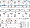 |
Fig. C.1. Graphical summary of the outcome of the IACOB-GBAT analysis for the O8 III((f)) star HD 36861, representative of the He-normal abundance group. The y-axis in the upper and lower set of panels correspond to the normalized flux and χ2, respectively. |
 |
Fig. C.2. Graphical summary of the outcome of the IACOB-GBAT analysis for the O7.5 III(f) star HD 34656, representative of the He-rich abundance group. |
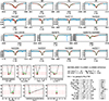 |
Fig. C.3. Graphical summary of the results of the IACOB-GBAT analysis for the O7 V((f))z star HD 47839, representative of the He-poor abundance group. Although not detected in the optical spectrum or through radial-velocity (RV) measurements (the peak-to-peak RV dispersion measured from 109 spectra in the IACOB spectroscopic database, spanning nearly nine years, is only 3.4 km s−1, Simón-Díaz et al. 2024), HD 47839 is known to be a long-period binary system (∼25 yr, Gies et al. 1997), including a fast-rotating B-type companion (see also Burssens et al. 2020). |
All Tables
Diagnostic lines used in the IACOB-GBAT spectroscopic analysis of our sample of Galactic O-type stars.
Stars in common with several studies in the literature for which we obtain discrepancies larger than 25% in the estimated He abundances.
All Figures
|
Fig. 1. He abundance distributions for the three groups of stars introduced in Sect. 4.1. The vertical dotted line indicates the present-day cosmic reference value provided by Nieva & Przybilla (2012). The black dot and horizontal line indicate the mean and standard deviation associated with Group 1 stars. |
| In the text | |
|
Fig. 2. Comparison of He abundances for a sample of 67 stars in common with the literature and 48 stars independently analysed for this work using the code MAUI. The open symbols refer to stars for which we have provided a Q2 or Q3 quality flag to the FASTWIND fits (see Tables D.1 to D.3). The 1-to-1 relation and 25% tolerance region are shown as dashed and dotted lines, respectively. The cross in the top left corner indicates the typical uncertainties in the YHe estimates. |
| In the text | |
|
Fig. 3. Distribution of the 318 Galactic O-type stars in a modified Hunter diagram, using He abundance instead of nitrogen on the y-axis. The fractions of He-rich stars in the slow- and fast-rotating subsamples are indicated, assuming v sin i = 200 km s−1 as the dividing threshold. ON, SB1, and RW stars are indicated with red small circles, blue crosses, and grey circles, respectively. |
| In the text | |
|
Fig. 4. Distribution of our sample of 318 Galactic O-type stars in a sHRD separated by the three He abundance groups described in Sect. 4.1. Evolutionary tracks from Ekström et al. (2012) for an initial spin rate vini/vcrit = 0.4 are depicted for reference purposes, highlighting in green the sections of the tracks where the He surface abundance reaches over 1.3 times the initial abundance. The symbols are the same as in Fig. 3. |
| In the text | |
|
Fig. 5. Distribution in the sHRD of the birth location of mass gainers as predicted by the binary evolution computations by Jin et al. (2026). The full sample of gainers are depicted in grey, while those with enriched He abundances are highlighted with colours separating the mass-transfer cases A (red), B (orange), and AB (blue). Single star evolutionary tracks computed with the MESA stellar evolution code by Jin et al. (2024a) and used as the basis for the binary evolution computation are also depicted for reference purposes. The open circles show the location of the He-rich group of O-type stars from our study. |
| In the text | |
|
Fig. A.1. Study of the impact of certain assumptions in the IACOB-GBAT analysis |
| In the text | |
|
Fig. C.1. Graphical summary of the outcome of the IACOB-GBAT analysis for the O8 III((f)) star HD 36861, representative of the He-normal abundance group. The y-axis in the upper and lower set of panels correspond to the normalized flux and χ2, respectively. |
| In the text | |
|
Fig. C.2. Graphical summary of the outcome of the IACOB-GBAT analysis for the O7.5 III(f) star HD 34656, representative of the He-rich abundance group. |
| In the text | |
|
Fig. C.3. Graphical summary of the results of the IACOB-GBAT analysis for the O7 V((f))z star HD 47839, representative of the He-poor abundance group. Although not detected in the optical spectrum or through radial-velocity (RV) measurements (the peak-to-peak RV dispersion measured from 109 spectra in the IACOB spectroscopic database, spanning nearly nine years, is only 3.4 km s−1, Simón-Díaz et al. 2024), HD 47839 is known to be a long-period binary system (∼25 yr, Gies et al. 1997), including a fast-rotating B-type companion (see also Burssens et al. 2020). |
| In the text | |
Current usage metrics show cumulative count of Article Views (full-text article views including HTML views, PDF and ePub downloads, according to the available data) and Abstracts Views on Vision4Press platform.
Data correspond to usage on the plateform after 2015. The current usage metrics is available 48-96 hours after online publication and is updated daily on week days.
Initial download of the metrics may take a while.