| Issue |
A&A
Volume 709, May 2026
|
|
|---|---|---|
| Article Number | A232 | |
| Number of page(s) | 9 | |
| Section | Planets, planetary systems, and small bodies | |
| DOI | https://doi.org/10.1051/0004-6361/202557868 | |
| Published online | 19 May 2026 | |
Electron temperatures in the ionosphere of Venus from Solar Orbiter/Radio and Plasma Waves instrument
1
Radboud Radio Lab, Department of Astrophysics, Radboud University
Nijmegen,
The Netherlands
2
LIRA, Observatoire de Paris, Université PSL, Sorbonne Université, Université Paris Cité, CY Cergy Paris Université, CNRS,
92190
Meudon,
France
3
Department of Physics, Imperial College London, South Kensington Campus,
London
SW7 2AZ,
UK
4
Swedish Institute of Space Physics (IRF),
Uppsala,
Sweden
5
Department of Physics and Astronomy, Uppsala University,
Uppsala
75121,
Sweden
6
Institute of Atmospheric Physics of the Czech Academy of Sciences,
Prague,
Czech Republic
7
LPP, CNRS, Ecole Polytechnique, Sorbonne Université, Observatoire de Paris, Université Paris-Saclay, Palaiseau,
Paris,
France
8
LPC2E, UMR7328 CNRS, OSUC, University of Orléans, CNRS, CNES,
Orléans,
France
9
Space Sciences Laboratory, University of California,
Berkeley,
CA,
USA
10
Physics Department, University of California,
Berkeley,
CA,
USA
★ Corresponding author: This email address is being protected from spambots. You need JavaScript enabled to view it.
Received:
28
October
2025
Accepted:
8
March
2026
Abstract
Context. On February 18, 2025, Solar Orbiter (SO) completed its fourth gravity assist maneuver of Venus (VGAM4) and reached an unprecedented proximity coming within 378 km of the planet. This flyby was necessary to steer the spacecraft into an orbit outside the plane of the ecliptic. Near the closest approach, only the Radio and Plasma Wave (RPW) and Magnetometer (MAG) instruments were operational; this enabled high-cadence measurements to be taken to investigate the plasma properties of the Venusian ionosphere.
Aims. The main goal of this study is to derive the electron density and temperature in the ionosphere of Venus using electric potential measurements from RPW, and to characterize them.
Methods. During approximately five minutes around the closest approach, the High Frequency Receiver of RPW detected radio emissions of a type naturally generated by planetary ionospheres whose frequency can be related to the electron density. Using quasithermal noise spectroscopy, we inferred the electron temperature at discrete altitudes and solar zenith angles.
Results. Solar Orbiter measured an average density and electron temperature in the ionosphere of Venus of 12 385 ± 148 cm−3 and 0.43 ± 0.05 eV, respectively. These values are in agreement with in-situ measurements by Pioneer Venus Orbiter (PVO) obtained at the solar maximum. Binned magnetic fields and temperatures are anticorrelated, which suggests that the magnetic flux ropes, observed in the Venus ionosphere, are more likely non-force-free structures.
Conclusions. The findings presented in this paper, together with the measurement from the Parker Solar Probe (PSP) during the third gravity assist, support the conclusion that the plasma density in the Venusian ionosphere above 350 km varies with solar activity, whereas the electron temperature shows a much weaker dependence. Notably, the electron temperature remains consistent across the three missions (SO, PSP, and PVO), despite varying levels of solar activity. This suggests that, over the altitude and solar zenith regions probed, the thermal structure of the Venusian ionosphere is not driven by solar extreme ultraviolet (EUV) heating alone, but is also shaped by external heat sources near the ionopause. Processes such as the damping of whistler mode waves, solar wind ion heating, and thermal conduction from the hot ionosheath appear to play a major role.
Key words: plasmas / methods: data analysis / planets and satellites: atmospheres / planets and satellites: individual: Venus
© The Authors 2026
 Open Access article, published by EDP Sciences, under the terms of the Creative Commons Attribution License (https://creativecommons.org/licenses/by/4.0), which permits unrestricted use, distribution, and reproduction in any medium, provided the original work is properly cited.
This article is published in open access under the Subscribe to Open model. This email address is being protected from spambots. You need JavaScript enabled to view it. to support open access publication.
1 Introduction
Although electron density and temperature measurements above ~250 km in the Venusian ionosphere have been reported (e.g. Theis et al. 1984), they are less abundant and exhibit greater variability than the extensive datasets available at lower altitudes. The existing in-situ observations are mostly from the NASA Pioneer Venus Orbiter (PVO) mission (Brace et al. 1979). Flybys of Venus by missions en route to other celestial bodies offer valuable opportunities to measure and or estimate upper-ionosphere and magnetosphere properties. However, since the measurements are based on a limited number of flybys or orbital passes, their space-time coverage is sparse or episodic. Recently, several spacecraft (Solar Orbiter, Parker Solar Probe, Bepi Colombo) have provided electron or plasma density measurements during flybys (e.g Hadid et al. 2021; Collinson et al. 2022; Persson et al. 2022; Edberg et al. 2024). Notably, only the NASA Parker Solar Probe (PSP) entered the Venusian ionosphere during its third (VGA3) and fourth (VGA4) Venus gravity assists. Although the electrostatic analyzers of the Solar Wind Electrons Alphas and Protons instrument aboard PSP were turned on, the ionospheric electrons are too cold and below the measurement energy threshold. Electron densities and temperatures were then estimated from plasma frequency measurements and using quasi-thermal noise (QTN) spectroscopy (Collinson et al. 2021; Tannous et al. 2024). These measurements, which were obtained near solar minimum, indicate a dependence on the solar cycle, as reduced electron densities were observed compared to PVO measurements acquired at solar maximum.
Eight Venus gravity assist maneuvers (VGAMs) are planned for the Solar Orbiter (SO) mission (Müller et al. 2020; Zouganelis et al. 2020), four of which have already been completed. The fourth VGAM occurred on February 18, 2025 when SO reached an unprecedented proximity to Venus entering the ionosphere. During VGAM4 SO approached from the Venus night side, thus passing into the shadow of the planet. In this region, cold ionospheric electrons constitute the dominant population, since the solar wind is excluded by the Venusian ionopause.
In this paper, we present the electron density and temperature in the Venusian ionosphere derived from electric power spectral density observations by the Radio and Plasma Waves (RPW) instrument aboard SO. We characterize these parameters and discuss their relation to other in situ measurements. Finally, we examine the relationship between the electron temperature and the magnetic field intensity measured by the SO magnetometer (MAG).
2 Overview of the Solar Orbiter VGAM4
Solar Orbiter entered the Venus-induced magnetosphere on the nightside northern hemisphere on February 18, 2025. It entered the Venus ionosphere near 20:45 UTC and exited around 20:50 UTC. The closest approach (CA) occurred around 20:48:45 in the proximity of the north pole at an altitude of 378 km. SO crossed the bow shock outbound around 20:54 UTC and continued upstream in the solar wind. The trajectory of the spacecraft in Venus Solar Orbital (VSO) coordinates is shown in Fig. 1. The VSO system is analogous to the geocentric solar ecliptic system (GSE) where XVSO is directed from the center of the planet toward the Sun, ZVSO is normal to the Venus orbital plane and positive toward the north celestial pole, and YVSO is positive in the direction opposite to orbital motion. The bow shock and induced magnetosphere boundary (also known as the upper mantle boundary) models from Martinecz et al. (2009) are also shown to indicate the approximate locations of SO encounters with these boundaries. Figure 2 (upper panel) shows a time series of the magnetic field intensity, measured by MAG, over approximately 15 minutes around the CA. The various regions encountered by SO during the flyby are indicated by colored bands. The ionopause crossing is marked by a sharp drop in the magnetic field intensity, after which SO enters the Venusian ionosphere for the first time. Although the magnetic field strength in the ionosphere is lower than in the induced magnetosphere, sharp magnetic field spikes, interpreted as magnetic flux ropes, are observed. An even sharper transition in the magnetic field delineates the outbound ionopause boundary at around 20:51 UTC. Subsequently, SO crosses the outbound dayside magnetosheath and the quasi-perpendicular bow shock before returning to the solar wind. For a complete description of these regions during the SO VGAM4 crossing see Edberg et al. (2026).
3 Solar Orbiter instruments operating during VGAM4
The RPW instrument (Maksimovic et al. 2020a) and the magnetometer MAG (Horbury et al. 2020a) were the only operating experiments during the flyby. RPW is designed to measure magnetic and electric fields and plasma wave spectra, as well as the spacecraft floating potential and radio emissions at frequencies up to 16 MHz. The three RPW electric antennas measure the electric field over a broad frequency range from DC to 16 MHz through the combined operation of four receivers that cover different frequency ranges. This configuration encompasses all relevant wave modes, from the magnetohydrodynamic regime through whistler and Langmuir waves to solar radio emissions. RPW measurements also enable the spacecraft potential relative to the surrounding plasma to be determined. In the magnetic domain, RPW has been designed to measure three-component magnetic field fluctuations, through a search-coil magnetometer (SCM, Jannet et al. 2021), over the frequency range 3 Hz to 1 MHz; this enables a full characterization of the magnetized plasma waves across this band. During VGAM4, SCM was kept off for safety reasons in order to mitigate the risk associated with the expected high temperatures.
In this paper, we focus on the data from the highest-frequency receiver of RPW, the High Frequency Receiver (HFR, Maksimovic et al. 2020a; Vecchio et al. 2021), which provides electric power spectral densities in the range 375 kHz-16 MHz, as well as data from MAG. The HFR is a sweeping receiver that operates exclusively in pseudo-dipole mode, which means it measures the potential difference between two monopole antennas. The three monopole sensors of RPW are named V1, V2, and V3 and correspond to the antennas Pz, Py, and My, respectively (see Fig. 7 from Maksimovic et al. 2020a). During the entire day of February 18, 2025, HFR was configured in a high time resolution mode, sweeping over 50 frequency steps between 425 kHz and ~16 MHz (not equispaced) and sampling the V1–V2 dipole antenna only. This configuration enabled a very high time cadence of ~1 s to be reached. Unfortunately, on the same day, data from the RPW Thermal Noise Receiver (TNR), which captures electric and magnetic power spectral densities in the 4 kHz–1 MHz range, were not available due to operational issues. During VGAM4, MAG provided vector magnetic field measurements at 128 Hz resolution.
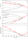 |
Fig. 1 Solar Orbiter trajectory (red) projected into the VSO XZ (a), XY planes (b) and in cylindrical coordinates (c). The bow shock (black dashed line) and the induced magnetospheric boundary (gray dashed line) from Martinecz et al. (2009) are also shown. |
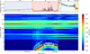 |
Fig. 2 Upper panel: magnetic field magnitude as a function of time around the CA to Venus. The different plasma regions are indicated by the colored bands: IM – induced magnetosphere; IP – ionopause; IS – ionosphere; MS – magnetosheath; BS – bow shock; SW – solar wind. The vertical dash-dot line marks the CA time. Lower panel: dynamic spectrum of the HFR power spectral density expressed in dB(V2/Hz). |
4 The RPW/HFR dataset
In this study, we considered the HFR power spectral densities, in V2/Hz from calibrated level 2 (L2) data (Maksimovic et al. 2020b). The lower panel of Fig. 2 shows the HFR data around the closest Venus approach. The strong signal, between 1–4 MHz, underlines the upper hybrid resonance emission (UH), which is visible whenever the measuring antenna is longer than the local Debye length. The UH frequency changes over time because of the varying distance from the planet. It increases during the SO approach and decreases during the outbound trajectory, reaching its maximum value at the time of minimum distance from the surface of Venus. The first order harmonic is visible at values 2ωUH following the time-frequency pattern of the UH peak. This effect is caused by the HFR electronic chain in the presence of the very high intensity signal produced at ωUH. The power excess at 2ωUH is thus not physically meaningful, but is just caused by instrumental effects.
The pixelated, stair-step appearance of the UH peak time profile arises from the combination of the HFR bandpass filter profile and the rapid drift of the UH frequency caused by the spacecraft inbound and outbound motion. This effect reduces the effective frequency resolution, which in turn limits the temporal resolution at which density and temperature measurements can be obtained. A more detailed discussion is presented in Appendix A.
5 Methods
5.1 Electron density
The local electron density, ne, can be derived from the measured frequency of the UH emission peak by combining the UH frequency with the electron cyclotron frequency, Ωce, to calculate the local plasma frequency, ωpe, (Eq. (1)):
![Mathematical equation: $\[\omega_{U H}=\sqrt{\omega_{p e}^2+\Omega_{c e}^2}\]$](/articles/aa/full_html/2026/05/aa57868-25/aa57868-25-eq1.png) (1)
(1)
where
![Mathematical equation: $\[\Omega_{c e}=\frac{e|B|}{m_e},\]$](/articles/aa/full_html/2026/05/aa57868-25/aa57868-25-eq2.png) (2)
(2)
MAG measurements indicate an average magnetic field strength in the Venusian ionosphere of 4.5 ± 5.1 nT, which corresponds to an electron cyclotron frequency on the order of 100–300 Hz. The Ωce term in Eq. (1) thus represents only a small correction (approximately 0.12% of ωUH) and can be neglected in the calculation of ne. By approximating ωpe~ωUH, we can directly derive ne from the HFR measured frequency of the UH emission peak, using the definition of plasma frequency
![Mathematical equation: $\[\omega_{U H} \sim \omega_{p e}=\sqrt{\frac{n_e e^2}{m_e \epsilon_0}}\]$](/articles/aa/full_html/2026/05/aa57868-25/aa57868-25-eq3.png) (3)
(3)
where ϵ0 is the permittivity of free space. From this ne derivation, it is possible to obtain the density at a higher time resolution than the HFR one by using the ne-probe-to-spacecraft potential measurements (Edberg et al. 2026).
5.2 Electron temperature
When the Debye length of the plasma is shorter than the antenna length, a clear QTN spectra, which results from the thermal motion of electrons and ions within the plasma near the spacecraft, is usually observed. Under these conditions, QTN spectroscopy offers an effective tool for measuring electron temperature and density by analyzing electrostatic fluctuations induced on an antenna by the thermal motion of surrounding plasma particles (Meyer-Vernet & Perche 1989). The standard method to estimate electron moments involves fitting observed spectral properties with parameters derived from a modeled electron velocity distribution (Issautier et al. 1998). Due to the low frequency resolution of HFR spectra above 1 MHz, the typical characteristics of the QTN spectrum (thermal plateau below ωpe, high-frequency spectrum above ωpe, shot noise generated by electron impacts below ωpe) are not visible and this approach is not fully feasible. We therefore implemented a different approach that consists in deriving the electron temperature by looking at the frequency and amplitude of the UH peak.
Two equations are useful for this purpose. The first expression provides the general definition of the Debye length in a plasma:
![Mathematical equation: $\[\lambda_D[m]=\sqrt{\frac{\epsilon_0 K_B T_e}{n_e e^2}} \sim \frac{0.07 \sqrt{T_e[K]}}{\sqrt{n_e\left[c m^{-3}\right]}}.\]$](/articles/aa/full_html/2026/05/aa57868-25/aa57868-25-eq4.png) (4)
(4)
This equation relates the local Debye length in the plasma to the electron temperature, Te.
The second equation, from Meyer-Vernet & Perche (1989),
![Mathematical equation: $\[V^2(\omega_{peak})[V^2 / H z] \sim 5 \cdot 10^{-16} T_e^{1 / 2}[K] \frac{\lambda_D}{L_{ant}}\left[\left(\frac{\omega_{p e}}{\Omega_{c e}}\right)^2-1\right]\]$](/articles/aa/full_html/2026/05/aa57868-25/aa57868-25-eq5.png) (5)
(5)
provides the peak power spectral density, V2, at a given time for Lant > λD and under conditions of weak magnetic fields, Ωce << ωpe. By deriving λD from Eq. (4), substituting into Eq. (5) and approximating (ωpe/Ωce)2 − 1 ~ (ωpe/Ωce)2 we get:
![Mathematical equation: $\[V^2\left(\omega_{p e a k}\right) \sim 5 \cdot 10^{-16} T_e \frac{0.07}{L_{a n t} \sqrt{n_e}}\left(\frac{\omega_{p e}}{\Omega_{c e}}\right)^2\]$](/articles/aa/full_html/2026/05/aa57868-25/aa57868-25-eq6.png) (6)
(6)
from which Te follows:
![Mathematical equation: $\[T_e=\frac{L_{a n t} V^2}{5 \cdot 10^{-16}} \frac{\sqrt{n_e}}{0.07}\left(\frac{\Omega_{c e}}{\omega_{p e}}\right)^2.\]$](/articles/aa/full_html/2026/05/aa57868-25/aa57868-25-eq7.png) (7)
(7)
The electron temperature, Te, can be calculated using ωpe (in place of ωUH) and V2(ωpeak) from HFR data, and Lant = 15.7 m (for the RPW V1–V2 dipole). Since the true peak value cannot be determined from the data due to the limited HFR bandwidth resolution (that caused the stair-step UH time profile) in Eq. (7), we used the maximum value of V2(ωpeak) for each frequency, which corresponds to the case where the plasma peak and the receiver filter were best aligned. Uncertainties on Te are obtained by error propagation through Eq. (7):
![Mathematical equation: $\[\delta T_e=\frac{L_{a n t} \Omega_{c e}^2}{5 \cdot 10^{-16}} \frac{1}{0.07}\]$](/articles/aa/full_html/2026/05/aa57868-25/aa57868-25-eq8.png) (8)
(8)
![Mathematical equation: $\[\left(\frac{\delta n_e}{2 \sqrt{n_e}} \cdot \frac{V^2}{\omega_{p e}^2}+\sqrt{n_e} \cdot \frac{\delta V^2}{\omega_{p e}^2}+\sqrt{n_e} \cdot V^2 \cdot \frac{2 \delta \omega_{p e}}{\omega_{p e}^3}\right).\]$](/articles/aa/full_html/2026/05/aa57868-25/aa57868-25-eq9.png) (9)
(9)
The values of the uncertainties in Equation (9) are the following:
δωpe: uncertainty in the determination of the plasma frequency due to the shape of the HFR bandpass filter. Details of the error calculation are provided in Appendix B;
δne = (meϵ0/e2) 2 ωpe δωpe, uncertainty in the electron density derived from HFR;
δV2: standard deviation of V2(ωpeak) for each value of ωUH.
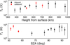 |
Fig. 3 Electron temperatures as derived from the RPW/HFR data for the inbound (black) and outbound (red) trajectories as a function of the distance from Venus’ surface (upper) and SZA (lower). Error bars correspond to the uncertainty derived from Eq. (9). |
6 Results
Figure 3 shows the HFR-derived electron temperatures as a function of height from Venus’ surface and of the solar zenith angle (SZA). The values of Te range between ~2500–8000 K. On the one hand, the electron temperature varies with altitude and reaches higher values at greater heights, with the upward trend continuing to approximately 850 km (upper panel). These findings are consistent with the general increase in electron temperature with altitude observed by PVO from 150 to 800 km (Knudsen et al. 1979a; Miller et al. 1980). The increase in Te with altitude is driven by a decreasing efficiency of electron-neutral cooling and thermal conduction, which balance heating sources within the ionosphere and at its topside. On the other hand, Te does not exhibit any clear correlation with SZA (lower panel) within the investigated range of altitude (>350 km) and SZA (50–90 deg) (Fig. 3, lower panel). These results are consistent with the lack of SZA dependence reported from the PVO measurements (Brace et al. 1979; Miller et al. 1980; Theis et al. 1984).
In the Venusian ionosphere, the electron temperature profile as a function of altitude results from the balance between heating processes, cooling through collisions with neutrals (and, to a lesser extent, ions), and thermal conduction. At high altitudes, where the collisional mean free path exceeds the electron temperature scale height, the classical conductive heat flux becomes invalid and must be replaced by a flux-limited formulation (Merritt & Thompson 1980). Energy sources include suprathermal photoelectrons, produced through solar EUV and X-ray deposition, which heat the ionospheric electrons through Coulomb collisions. Previous studies have shown that solar heating alone cannot account for the electron temperatures observed by PVO, which indicates that external heating sources are required in the topside ionosphere (Knudsen et al. 1979b, 1980; Cravens et al. 1980, 1981; Brace & Kliore 1991). The presence of an additional energy source would also account for the lack of SZA dependence of Te. While an increase in solar activity has a negative feedback on Te, as at solar maximum more electrons are produced and it requires more energy to heat the entire population, it would attenuate the SZA dependence of Te but not hide it.
The electron density from HFR is shown as a function of height and SZA in Fig 4. The comparison between the two plots in Fig. 4 reveals that the ionospheric plasma structure during the flyby is driven by both variations in height and SZA. Density increases as SO was approaching the surface of Venus, varying from about 18 500 cm−3 at the minimum distance of ~378 km to 2200 cm−3 at about 1000 km, as SO was above the plasma density peak typically around 140–150 km for the range of SZA probed (Fox 2007). However, the density values at the same height are different for the inbound and outbound paths due to the difference in SZA. The electron density on the sunlit side is driven by the ionization of the upper atmosphere by solar EUV radiation (Miller et al. 1980; Fox 2007; Peter et al. 2014; Tripathi et al. 2023; Ambili et al. 2024). Consequently, the plasma density increases from the terminator (90°) to solar noon. At a given altitude, the plasma density is higher during the outbound path (SZA<60°) than during the inbound path (SZA>60°). During the inbound phase, both SZA and altitude decrease, resulting in a clear increase in plasma density. The density increase is particularly significant as SO was crossing the solar terminator where the variations in plasma density with solar zenith angle are the strongest (Theis et al. 1984; Fox 2007; Peter et al. 2014; Tripathi et al. 2023; Ambili et al. 2024). In contrast, during the outbound phase, SZA continues to decrease, while the altitude increases, which leads to an ambiguous temporal trend due to these opposing variations.
Figure 5 shows a representation of the density and temperature variations as a function of altitude above Venus’ surface and SZA, where the symbol size is proportional to the measured temperature and density normalized to their respective maximum values. This visualization emphasizes that Te is primarily controlled by altitude, whereas ne is influenced by both altitude and SZA. The size of the temperature markers (red squares) increases with altitude, while the plasma density marker size (black dots) increases from the terminator at high altitude, toward noon and lower altitude during the inbound path.
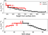 |
Fig. 4 Electron density as derived from the RPW/HFR data for the inbound (black) and outbound (red) trajectories as a function of the distance from Venus’ surface (upper) and SZA (lower). Error bars represent the uncertainty discussed in the main text. |
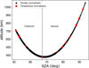 |
Fig. 5 Electron density (black dot) and temperature (red square), normalized to their maximum values, as a function of the SZA and altitude. The size of the marker is proportional to the values of electron density and temperature. The dashed line indicates the CA. |
7 Comparison with PVO and PSP measurements
Electron temperatures in the Venusian ionosphere were measured in-situ, in the 1978–1992 interval, by the Orbiter Electron Temperature Langmuir probe (OETP) instrument (Brace et al. 1979; Brace & Theis 2024) aboard the NASA Pioneer Venus Orbiter mission. These measurements were taken in the ionosphere only during the solar maximum 1979–1980 and before the atmospheric burning up in 1992. PVO temperatures measured during the periods January 1, 2025-January 1, 1983 and October 7, 1989-October 7, 1992, both near solar maximum, are shown in Fig. 6 (black dots) as a function of altitude above Venus’ surface (upper panel) and SZA (lower panel). HFR temperatures (light blue squares) overlap well with the OETP measurements. To allow a more quantitative comparison between the two datasets, we binned the OETP measurements. In the upper panel, OETP data are grouped by altitude above Venus’ surface using 50 km bins centered on the SO average altitude corresponding to each HFR Te measurement. Two cases are shown: (1) median temperatures for all OETP data within each altitude bin, independent of latitude and longitude (yellow crosses); and (2) median temperatures within a 30° × 30° cell centered on the average SO coordinates in the corresponding altitude bin (magenta dots). In the lower panel, median OETP temperatures are computed over 50 km altitude and 1.5° SZA bins (magenta dots). The temperatures derived from HFR measurements and the OETP median values are consistent within the uncertainties. Temperature variations as a function of SZA exhibit a similar pattern for both HFR and median PVO data, which indicates a weak dependence on SZA. The observed temperature variations are mainly due to differences in altitude rather than SZA variations. For instance, the temperature dip near 68° in the HFR data corresponds to the point of closest approach along the spacecraft trajectory and is expected to coincide with the lowest electron temperature. This dip is still visible in the PVO binned data, although it is less pronounced. The reduced amplitude arises because each PVO data point represents the median value within a 50 km altitude bin, which smooths out local altitude-dependent variations. Consequently, the altitude effect remains evident but appears attenuated due to the binning.
The average electron temperature measured by PSP near solar minimum during VGA3, Te = 4294 ± 464 K (red symbol) at closest approach (~ 880 Km and SZA=136°, Collinson et al. 2021; Tannous et al. 2024), is also shown in the upper panel. This value is consistent with those obtained from SO and PVO measurements at comparable altitudes, despite the difference in solar activity.
Figure 7 compares the electron density and temperature pairs derived from HFR and OETP measurements during solar maxima. To match the number of points with Te, HFR densities were downsampled by taking a single value for each ”step” in the ne profile shown in Fig. 4. Small dots represent all PVO measurements obtained within the same time interval as in Fig. 6, binned into 50 km × 1.5° cells in the altitude-SZA space and centered on the corresponding HFR measurement values. Large dots show the median value within each cell, while the color scale denotes the bin centers. Although some HFR points, particularly along the outbound trajectory, lie near the edges of the PVO measurement distribution, the Te–ne pairs from OETP and HFR remain consistent within the measurement uncertainties. A decreasing trend in temperature with increasing density is evident despite the scatter in HFR points. The color trend, which reflects SZA and altitude, is consistent between SO/HFR and PVO/OETP measurements. A PSP VGA3 data point (red) is also shown in Fig. 7. In the Te–ne plane the PSP measurement is clearly separated from the PVO and SO data pairs, which reflects the very low plasma densities observed under solar minimum conditions. These results are consistent with previously reported solar cycle–related variations in the plasma structure of the Venusian ionosphere (e.g., Fox & Sung 2001; Collinson et al. 2021).
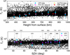 |
Fig. 6 In-situ electron temperatures measured by PVO/OETP during January 1, 2025–January 1, 1983 and October 7, 1989–October 7, 1992 intervals (black dots). Electron temperatures derived from SO/RPW/HFR data (light-blue squares). Upper: colored symbols correspond to median PVO/OETP temperatures computed over 50 km altitude bins for the full dataset (yellow crosses) and within a 30° × 30° cell centered on the average SO latitude and longitude in the VSO frame (magenta dots). The red diamond marks the average temperature measured by PSP during VGA3 (Tannous et al. 2024). Lower: median PVO/OETP temperatures calculated over 50 km altitude bins and 1.5° SZA intervals (magenta dots). Numbers above the colored markers indicate the altitude at the center of each bin. The average electron temperature measured by PSP is outside the x-axis range of the current plot (SZA=136°) and is not shown. The error bars of the binned OETP measurements represent the total uncertainty, including both statistical and systematic contributions. The statistical contribution is given by the standard error of the sample mean (defined as the sample standard deviation, σ, divided by the square root of the sample size, N) while a 5% systematic uncertainty is assumed (Theis 1993). |
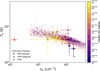 |
Fig. 7 Electron density, ne, and temperature, Te, pairs as derived from RPW/HFR (squares: inbound; triangles: outbound) and measured by PVO/OETP (small dots) in 50 km × 1.5° altitude-SZA cells centered on each HFR measurement. Large dots correspond to the median values in each cell. The red diamond marks the PSP measurement (ne = 144 ± 37 cm−3, Te = 4294 ± 464 K, Tannous et al. 2024) during the VGA3 at about 830 km from Venus’ surface. The HFR measurement at CA is also indicated. The color scale denotes the bin centers. The error bars of the binned OETP measurements represent the total uncertainty, including both statistical and systematic contributions. The statistical contribution is given by the standard error of the sample mean while systematic uncertainties of 5% and 10% are assumed for temperature and density, respectively (Theis 1993). |
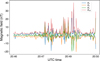 |
Fig. 8 Magnetic field components in the VSO frame and the total magnetic field acquired by MAG in the Venusian ionosphere. |
8 Comparison with MAG measurements
Magnetic field intensities (Horbury et al. 2020b) measured by MAG in the Venusian ionosphere are shown in Fig. 8 in the VSO frame. The spikes observed in all magnetic field components correspond to small-scale structures known as magnetic flux ropes. These flux ropes, which carry the solar wind field and plasma tailward, were previously observed in the near-Venus space environment by the PVO (Russell et al. 1990; Luhmann & Cravens 1991; Ledvina et al. 2002) and Venus Express (VEX, Zhang et al. 2012; Chen et al. 2017) missions. A more comprehensive analysis of the magnetic flux ropes detected by SO during VGAM4 and a comparison with high-resolution (4096 Hz) density data from RPW are provided in Edberg et al. (2026). Here, we restrict ourselves to a qualitative discussion of the potential relationship between temperatures derived from HFR measurements and magnetic fields observed by MAG. Due to an unsatisfactory time resolution of the electron temperature, a direct comparison of B − Te within a flux rope is not possible. To investigate potential statistical correlations, we compared electron temperatures with binned magnetic field measurements. For this purpose, we computed the mean magnetic field magnitude within time bins centered on ti, with half-widths given by (ti − ti–1)/2 and (ti+1 − ti)/2. The comparison is shown in Fig. 9. The Te and binned Bmod curves show a clear anticorrelation, that extends beyond the lower-altitude region where lower temperatures are expected. The Pearson correlation coefficient calculated for the two curves is −0.82, with a very low probability of 0.006 that the observed correlation occurred by chance. This result suggests that the temperature is generally lower in the entire region where the magnetic field is stronger (and therefore where there is a larger number of flux ropes). This further suggests that the temperature inside the flux ropes would be lower than in the surrounding plasma, where the magnetic field is weaker, pointing toward the non-force-free nature of the observed flux ropes (Elphic et al. 1981). The results discussed above are consistent with the results of Ledvina et al. (2002), who analyzed magnetic and thermal pressure variations in ~2300 flux ropes observed by PVO. They found that at higher altitudes (>250 km) flux ropes exhibit a significant non-force-free component, with reduced plasma pressure inside the ropes relative to the outside to balance the magnetic pressure.
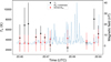 |
Fig. 9 Electron temperatures derived from SO/RPW/HFR data (black), compared with SZA-binned (red) and full (blue) SO/MAG magnetic field intensity data, plotted as a function of time. |
9 Conclusions
We considered electric power spectral density data (in units of V2/Hz) from the RPW/HFR receiver during the SO VGAM4, and used UH frequency measurements and QTN theory to derive the electron density and temperature in the ionosphere of Venus. Overall, the measured density and electron temperature are consistent with in-situ measurements by PVO during the epochs of maxima of the solar activity in terms of intensity and spatial variations. We also detected a decreasing trend in temperature with increasing density, as expected from PVO measurements. Variations in electron density are strongly controlled by the SZA and altitude. Along the inbound path, decreasing SZA and altitude lead to an increase in plasma density, which reflects enhanced ionization in regions exposed to solar EUV radiation (Miller et al. 1980; Fox 2007). In contrast, the electron temperature shows a lack of correlation with SZA; it mainly varies with altitude and reaches higher values at greater heights, which is consistent with early PVO observations (Brace et al. 1979; Miller et al. 1980; Theis et al. 1984).
Observations from PSP during VGA3 at solar minimum show reduced plasma densities compared to PVO and SO measurements taken near solar maximum (Collinson et al. 2021; Tannous et al. 2024), while the PSP electron temperatures are consistent with those observed by PVO and SO. These findings, together with the results of this study, support the notion that, in the altitude range relevant to the observations (above ~350 km), the global plasma density structure of the Venusian ionosphere varies over the 11-year solar activity cycle, while the electron temperature appears to be much less sensitive to solar illumination and activity (within the uncertainties of the measurements and the range of SZA probed). The dependence of ne on solar activity is also consistent with radio occultation measurements near solar minimum from VEX (Peter et al. 2025) and Akatsuki (Tripathi et al. 2023), which indicates that the Venusian ionosphere exhibits a reduced total electron content relative to periods of higher solar activity. Our results therefore suggest that the ionospheric thermal structure is not driven by solar EUV heating alone. This interpretation is consistent with earlier observations and modeling studies of the Venusian ionosphere. Field-free thermal ionospheric models driven by solar heating alone underestimate the electron temperatures measured by PVO, which indicates that additional physical processes are required (Knudsen et al. 1979b, 1980; Cravens et al. 1980, 1981; Brace & Kliore 1991). The presence of a quasi-horizontal, fluctuating magnetic field would reduce the thermal conductivity and hence increase Te. However, a large part of the region probed by SO is nearly field free (see Fig. 8). The most likely explanation for the high values in electron temperature and lack of dependence on SZA and solar activity is the presence of an external heat source near the ionopause, such as the damping of whistler mode waves, solar wind ion heating, and thermal conduction from the hot ionosheath (e.g. Cravens et al. 1980, 1981).
Finally, we provided a comparison between the magnetic field and temperatures, which, albeit indirectly, provide hints about the nature of magnetic flux ropes observed in the Venusian ionosphere. This comparison indicates an anticorrelation between magnetic field intensity and temperature that suggests that the magnetic flux ropes, observed by SO above the altitude of ~350 km, can be compatible with non-force-free structures. These findings are consistent with those of Edberg et al. (2026), who investigated magnetic flux ropes during VGAM4 using high-cadence electron density measurements derived from SO spacecraft potential. The high-cadence data suggest that the flux ropes were probably not pressure-balanced.
Acknowledgements
The Solar Orbiter data are available through ESA SOAR archive (https://soar.esac.esa.int/soar/). Solar Orbiter is a mission of international cooperation between ESA and NASA, operated by ESA. The RPW instrument has been designed and funded by CNES, CNRS, the Paris Observatory, The Swedish National Space Agency, ESA-PRODEX and all the participating institutes. The Solar Orbiter magnetometer was funded by the UK Space Agency (grant ST/T001062/1). D.P. and J.S. received support from the Czech Science Foundation grant no. 22-10775S.
References
- Ambili, K. M., Choudhary, R. K., & Tripathi, K. R. 2024, Icarus, 408, 115839 [Google Scholar]
- Brace, L. H., & Kliore, A. J. 1991, Space Sci. Rev., 55, 81 [NASA ADS] [CrossRef] [Google Scholar]
- Brace, L. H., & Theis, R. F. 2024, Pioneer Venus Orbiter Electron Temperature Probe (OETP) Data, NASA Planetary Data System, dataset available at NASA Planetary Data System [Google Scholar]
- Brace, L. H., Theis, R. F., Krehbiel, J. P., et al. 1979, Science, 203, 763 [Google Scholar]
- Chen, Y. Q., Zhang, T. L., Xiao, S. D., & Wang, G. Q. 2017, J. Geophys. Res. Space Phys., 122, 8858 [Google Scholar]
- Collinson, G. A., Ramstad, R., Glocer, A., Wilson, L., & Brosius, A. 2021, Geophys. Res. Lett., 48, e92243 [Google Scholar]
- Collinson, G. A., Ramstad, R., Frahm, R., et al. 2022, Geophys. Res. Lett., 49, e2021GL096485 [CrossRef] [Google Scholar]
- Cravens, T. E., Gombosi, T. I., Kozyra, J., et al. 1980, J. Geophys. Res., 85, 7778 [Google Scholar]
- Cravens, T. E., Nagy, A. F., & Gombosi, T. I. 1981, Adv. Space Res., 1, 33 [Google Scholar]
- Edberg, N. J. T., Andrews, D. J., Boldú, J. J., et al. 2024, J. Geophys. Res. (Space Phys.), 129, e2024JA032603 [Google Scholar]
- Edberg, N. J. T., Eriksson, A. I., Boldú, J. J., et al., 2026, J. Geophys. Res. (Space Phys.), 131, e2025JA034813 [Google Scholar]
- Elphic, R. C., Luhmann, J. G., Russell, C. T., & Brace, L. H. 1981, Adv. Space Res., 1, 53 [Google Scholar]
- Fox, J. L. 2007, J. Geophys. Res. Planets, 112, E04S02 [Google Scholar]
- Fox, J. L., & Sung, K. Y. 2001, J. Geophys. Res., 106, 21305 [NASA ADS] [CrossRef] [Google Scholar]
- Hadid, L. Z., Edberg, N. J. T., Chust, T., et al. 2021, A&A, 656, A18 [NASA ADS] [CrossRef] [EDP Sciences] [Google Scholar]
- Horbury, T. S., O’Brien, H., Carrasco Blazquez, I., et al. 2020a, A&A, 642, A9 [NASA ADS] [CrossRef] [EDP Sciences] [Google Scholar]
- Horbury, et al. 2020b, MAG, Solar Orbiter magnetometer, 1.0, European Space Agency, https://doi.org/10.5270/esa-ux7y320 [Google Scholar]
- Issautier, K., Meyer-Vernet, N., Moncuquet, M., & Hoang, S. 1998, J. Geophys. Res., 103, 1969 [NASA ADS] [CrossRef] [Google Scholar]
- Jannet, G., Dudok de Wit, T., Krasnoselskikh, V., et al. 2021, J. Geophys. Res. (Space Phys.), 126, e28543 [Google Scholar]
- Knudsen, W. C., Spenner, K., Michelson, P. F., et al. 1980, J. Geophys. Res., 85, 7754 [Google Scholar]
- Knudsen, W. C., Spenner, K., Whitten, R. C., et al. 1979a, Science, 203, 757 [Google Scholar]
- Knudsen, W. C., Spenner, K., Whitten, R. C., et al. 1979b, Science, 205, 105 [Google Scholar]
- Ledvina, S. A., Nunes, D. C., Cravens, T. E., & Tinker, J. L. 2002, J. Geophys. Res. (Space Phys.), 107, 1074 [Google Scholar]
- Luhmann, J. G., & Cravens, T. E. 1991, Space Sci. Rev., 55, 201 [Google Scholar]
- Maksimovic, M., Bale, S. D., Chust, T., et al. 2020a, A&A, 642, A12 [EDP Sciences] [Google Scholar]
- Maksimovic, M., et al. 2020b, RPW – Radio and Plasma Waves instrument, 1.0, European Space Agency, https://doi.org/10.57780/esa-3xcjd4w [Google Scholar]
- Martinecz, C., Boesswetter, A., FräNz, M., et al. 2009, J. Geophys. Res. (Planets), 114, E00B30 [Google Scholar]
- Merritt, D., & Thompson, K. 1980, J. Geophys. Res., 85, 6778 [Google Scholar]
- Meyer-Vernet, N., & Perche, C. 1989, J. Geophys. Res., 94, 2405 [NASA ADS] [CrossRef] [Google Scholar]
- Miller, K. L., Knudsen, C. W., Spenner, K., Whitten, R. C., & Novak, V. 1980, J. Geophys. Res., 85, 7759 [Google Scholar]
- Müller, D., Cyr, O. C. St., Zouganelis, I., et al. 2020, A&A, 642, A1 [NASA ADS] [CrossRef] [EDP Sciences] [Google Scholar]
- Persson, M., Aizawa, S., André, N., et al. 2022, Nat. Commun., 13, 7743 [NASA ADS] [CrossRef] [Google Scholar]
- Peter, K., Pätzold, M., Molina-Cuberos, G., et al. 2014, Icarus, 233, 66 [NASA ADS] [CrossRef] [Google Scholar]
- Peter, K., Pätzold, M., Withers, P., et al. 2025, Icarus, 432, 116469 [Google Scholar]
- Russell, C. T., Priest, E. R., & Lee, L. C. 1990, Geophys. Monogr. Ser., 58 [Google Scholar]
- Tannous, S. M., Bonnell, J. W., Pulupa, M., & Bale, S. D. 2024, Geophys. Res. Lett., 51, e2024GL110105 [Google Scholar]
- Theis, R. 1993, PVO Venus Electron Temperature Probe Derived Electron Density Low Resolution Version 1.0, NASA Planetary Data System, pVO-V-OETP-5-ELECTRONDENSITY-LORES-V1.0 [Google Scholar]
- Theis, R. F., Brace, L. H., Elphic, R. C., & Mayr, H. G. 1984, J. Geophys. Res., 89, 1477 [Google Scholar]
- Tripathi, K. R., Choudhary, R. K., Ambili, K. M., & Imamura, T. 2023, J. Geophys. Res. (Planets), 128, e2023JE007768 [Google Scholar]
- Vecchio, A., Maksimovic, M., Krupar, V., et al. 2021, A&A, 656, A33 [NASA ADS] [CrossRef] [EDP Sciences] [Google Scholar]
- Zhang, T. L., Baumjohann, W., Teh, W. L., et al. 2012, Geophys. Res. Lett., 39, L23103 [Google Scholar]
- Zouganelis, I., De Groof, A., Walsh, A. P., et al. 2020, A&A, 642, A3 [NASA ADS] [CrossRef] [EDP Sciences] [Google Scholar]
Appendix A Effect of the HFR filter shape
The HFR bandpass filter has a rectangular shape with a bandwidth of δfbw = 30 kHz. To increase the time cadence and exclude frequencies affected by electromagnetic interference, HFR was configured to sweep over a comb of 50 unequally spaced frequencies (see Table A.1). An example of the HFR bandwidth resulting from the combination of the shape of the filter and the comb of chosen frequencies is shown in Fig. A.1 (upper panel, blue line). Assuming a Gaussian-shaped spectrum for the external signal, whose peak drifts in frequency at a rate similar to that observed by HFR (Fig. A.1, upper panel, red curves), the convolution of the signal with the HFR bandwidth at each time produces the synthetic dynamic spectrum shown in Fig. A.1 (lower panel), successfully reproducing the main features of the observed spectrum in Fig. 2.
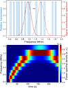 |
Fig. A.1 Upper: Relative transmission of the HFR filter resulting from the combination of the shape of the filter and the comb of chosen frequencies (blue lines). The Gaussian-shaped spectrum of the external signal is also shown (red lines). For sake of simplicity it peaks at 1. The solid and dotted lines refer to the spectrum of the external signal at two different time instants. The frequency drift of the spectrum over time is indicated by the arrow. Lower: synthetic HFR dynamic spectrum obtained by mimic the HFR response to an input frequency shifting Gaussian-shaped spectrum. |
The 50 center frequencies for bands sampled by HFR.
Appendix B Error in the determination of the plasma frequency
The uncertainty in the determination of ωp arises from the irregular comb-like response of the HFR filter, which implies that the frequency is not continuously sampled and that any detected peak frequency is quantized to the comb spacing. The uncertainty δωpe is therefore defined as
![Mathematical equation: $\[\delta \omega_{p e}=\sqrt{\left(\frac{\Delta f}{2}\right)^2+\left(\frac{\delta f_{b w}}{2}\right)^2}\]$](/articles/aa/full_html/2026/05/aa57868-25/aa57868-25-eq10.png) (B.1)
(B.1)
where Δf is the spacing between the center frequencies of adjacent comb teeth. Due to the non-uniform spacing of the HFR frequency sweep, Δf varies between about 50 and 200 kHz over the considered frequency range, with smaller spacings and therefore lower errors occurring at lower frequencies. As a result, δωpe ranges from about 30 to 200 kHz.
All Tables
All Figures
|
Fig. 1 Solar Orbiter trajectory (red) projected into the VSO XZ (a), XY planes (b) and in cylindrical coordinates (c). The bow shock (black dashed line) and the induced magnetospheric boundary (gray dashed line) from Martinecz et al. (2009) are also shown. |
| In the text | |
|
Fig. 2 Upper panel: magnetic field magnitude as a function of time around the CA to Venus. The different plasma regions are indicated by the colored bands: IM – induced magnetosphere; IP – ionopause; IS – ionosphere; MS – magnetosheath; BS – bow shock; SW – solar wind. The vertical dash-dot line marks the CA time. Lower panel: dynamic spectrum of the HFR power spectral density expressed in dB(V2/Hz). |
| In the text | |
|
Fig. 3 Electron temperatures as derived from the RPW/HFR data for the inbound (black) and outbound (red) trajectories as a function of the distance from Venus’ surface (upper) and SZA (lower). Error bars correspond to the uncertainty derived from Eq. (9). |
| In the text | |
|
Fig. 4 Electron density as derived from the RPW/HFR data for the inbound (black) and outbound (red) trajectories as a function of the distance from Venus’ surface (upper) and SZA (lower). Error bars represent the uncertainty discussed in the main text. |
| In the text | |
|
Fig. 5 Electron density (black dot) and temperature (red square), normalized to their maximum values, as a function of the SZA and altitude. The size of the marker is proportional to the values of electron density and temperature. The dashed line indicates the CA. |
| In the text | |
|
Fig. 6 In-situ electron temperatures measured by PVO/OETP during January 1, 2025–January 1, 1983 and October 7, 1989–October 7, 1992 intervals (black dots). Electron temperatures derived from SO/RPW/HFR data (light-blue squares). Upper: colored symbols correspond to median PVO/OETP temperatures computed over 50 km altitude bins for the full dataset (yellow crosses) and within a 30° × 30° cell centered on the average SO latitude and longitude in the VSO frame (magenta dots). The red diamond marks the average temperature measured by PSP during VGA3 (Tannous et al. 2024). Lower: median PVO/OETP temperatures calculated over 50 km altitude bins and 1.5° SZA intervals (magenta dots). Numbers above the colored markers indicate the altitude at the center of each bin. The average electron temperature measured by PSP is outside the x-axis range of the current plot (SZA=136°) and is not shown. The error bars of the binned OETP measurements represent the total uncertainty, including both statistical and systematic contributions. The statistical contribution is given by the standard error of the sample mean (defined as the sample standard deviation, σ, divided by the square root of the sample size, N) while a 5% systematic uncertainty is assumed (Theis 1993). |
| In the text | |
|
Fig. 7 Electron density, ne, and temperature, Te, pairs as derived from RPW/HFR (squares: inbound; triangles: outbound) and measured by PVO/OETP (small dots) in 50 km × 1.5° altitude-SZA cells centered on each HFR measurement. Large dots correspond to the median values in each cell. The red diamond marks the PSP measurement (ne = 144 ± 37 cm−3, Te = 4294 ± 464 K, Tannous et al. 2024) during the VGA3 at about 830 km from Venus’ surface. The HFR measurement at CA is also indicated. The color scale denotes the bin centers. The error bars of the binned OETP measurements represent the total uncertainty, including both statistical and systematic contributions. The statistical contribution is given by the standard error of the sample mean while systematic uncertainties of 5% and 10% are assumed for temperature and density, respectively (Theis 1993). |
| In the text | |
|
Fig. 8 Magnetic field components in the VSO frame and the total magnetic field acquired by MAG in the Venusian ionosphere. |
| In the text | |
|
Fig. 9 Electron temperatures derived from SO/RPW/HFR data (black), compared with SZA-binned (red) and full (blue) SO/MAG magnetic field intensity data, plotted as a function of time. |
| In the text | |
|
Fig. A.1 Upper: Relative transmission of the HFR filter resulting from the combination of the shape of the filter and the comb of chosen frequencies (blue lines). The Gaussian-shaped spectrum of the external signal is also shown (red lines). For sake of simplicity it peaks at 1. The solid and dotted lines refer to the spectrum of the external signal at two different time instants. The frequency drift of the spectrum over time is indicated by the arrow. Lower: synthetic HFR dynamic spectrum obtained by mimic the HFR response to an input frequency shifting Gaussian-shaped spectrum. |
| In the text | |
Current usage metrics show cumulative count of Article Views (full-text article views including HTML views, PDF and ePub downloads, according to the available data) and Abstracts Views on Vision4Press platform.
Data correspond to usage on the plateform after 2015. The current usage metrics is available 48-96 hours after online publication and is updated daily on week days.
Initial download of the metrics may take a while.