| Issue |
A&A
Volume 708, April 2026
|
|
|---|---|---|
| Article Number | A373 | |
| Number of page(s) | 18 | |
| Section | Extragalactic astronomy | |
| DOI | https://doi.org/10.1051/0004-6361/202555185 | |
| Published online | 28 April 2026 | |
The major merger–active galactic nucleus connection up to cosmic noon
1
SRON Netherlands Institute for Space Research, Landleven 12, 9747 AD, Groningen, The Netherlands
2
Kapteyn Astronomical Institute, University of Groningen, Postbus 800, 9700 AV, Groningen, The Netherlands
3
European Space Agency/ESTEC, Keplerlaan 1, 2201 AZ, Noordwijk, The Netherlands
4
Instituto de Radioastronomía y Astrofísica, Universidad Nacional Autónoma de México, A.P. 72-3, 58089, Morelia, Mexico
5
School of Physics and Astronomy, University of Nottingham, University Park, Nottingham, NG7 2RD, UK
★ Corresponding author: This email address is being protected from spambots. You need JavaScript enabled to view it.
Received:
16
April
2025
Accepted:
26
February
2026
Abstract
Galaxy major mergers are a potential mechanism for triggering active galactic nuclei (AGN) activity, but their role remains debated, particularly beyond the local Universe. We aim to shed light on the merger–AGN connection at z = 0.5–2, exploiting the multi-wavelength datasets and James Webb Space Telescope (JWST) observations in the COSMOS field. We construct a stellar mass-limited sample and identify AGN via mid-infrared (MIR) colours, X-ray detections, and spectral energy distribution (SED) fitting. We train convolutional neural networks to identify mergers with mock JWST observations. We create non-AGN and non-merger control samples matching the redshift, stellar mass, and star formation rate distributions of the AGN and mergers. We find AGN to be somewhat more frequent in mergers than in non-mergers, with excess ratios ranging from ∼2.5 (X-ray AGN) to ∼1.3 (MIR) and ∼1.1–1.2 (SED AGN). Similarly, AGN galaxies show a higher merger fraction (fmerg) than non-AGN controls. We then study fmerg as a function of relative and absolute AGN power, utilising the AGN fraction (fAGN) and accretion disc luminosity (Ldisc) parameters. We uncover a fmerg–fAGN relation with two regimes: fmerg stays roughly flat for less-dominant AGN (fAGN < 0.8) but increases at fAGN > 0.8 for the MIR and X-ray AGN, and more gently for SED AGN, where mergers appear to be the main triggering mechanism. Additionally, fmerg increases monotonically as a function of Ldisc, for all AGN types, reaching fmerg > 50% for the most luminous AGN (Ldisc ≳ 1046 erg s−1). Overall, our results suggest that major mergers can trigger AGN out to cosmic noon at z ∼ 2. Furthermore, the role of major mergers shows a clear dependence on AGN luminosity and remains the principal mechanism for fuelling the most powerful AGN.
Key words: techniques: image processing / galaxies: active / galaxies: evolution / galaxies: interactions
© The Authors 2026
 Open Access article, published by EDP Sciences, under the terms of the Creative Commons Attribution License (https://creativecommons.org/licenses/by/4.0), which permits unrestricted use, distribution, and reproduction in any medium, provided the original work is properly cited.
This article is published in open access under the Subscribe to Open model. This email address is being protected from spambots. You need JavaScript enabled to view it. to support open access publication.
1. Introduction
Under hierarchical structure formation, mergers play a crucial role in galaxy evolution. Mergers can contribute significantly to the stellar-mass assembly process as two or more galaxies collide and coalesce into a single, more massive galaxy (for a review, see Somerville & Davé 2015). During these interactions, gravity pulls and distorts the galaxies involved, changing their dynamics and morphology (Toomre & Toomre 1972; Conselice 2006). In addition, while rearranging the star and gas distributions, mergers have been observed to enhance star formation rates (SFRs; Martin et al. 2021; Bickley et al. 2022), to extreme levels in some cases (Mihos & Hernquist 1994; Cibinel et al. 2019). Mergers are also acknowledged as a viable mechanism for funnelling gas towards super-massive black holes (SMBHs; Hopkins et al. 2006; Blumenthal & Barnes 2018). Many simulations suggest that mergers can fuel accretion onto SMBHs, triggering active galactic nuclei (AGN; Di Matteo et al. 2005; Blecha et al. 2018), although others predict that mergers may be only a secondary path (Martin et al. 2018; Bhowmick et al. 2020; Byrne-Mamahit et al. 2023). Observational studies also find seemingly contradictory results. In the local Universe, some works support the scenario in which mergers trigger AGN (Urrutia et al. 2008; Hwang et al. 2012; Lackner et al. 2014; Goulding et al. 2018; Gao et al. 2020; Pierce et al. 2022), while others reject this picture (Reichard et al. 2009; Cisternas et al. 2011; Sabater et al. 2015; Smethurst et al. 2024). Higher-redshift studies, limited to much smaller samples, find similarly mixed results (Allevato et al. 2011; Kocevski et al. 2012, 2015; Mechtley et al. 2016; Fan et al. 2016; Marian et al. 2019; Silva et al. 2021; Bonaventura et al. 2025). Furthermore, some investigations reveal dependence on AGN luminosity and dust obscuration, indicating that mergers may be more important in triggering more luminous or dust-obscured AGN (Treister et al. 2012; Glikman et al. 2015; Ricci et al. 2017, 2021; Donley et al. 2018; Weigel et al. 2018; Ellison et al. 2019; Bickley et al. 2023; Euclid Collaboration: La Marca et al. 2026), although not all studies confirm these findings (Villforth et al. 2017; Hewlett et al. 2017).
The first issue in investigating the merger–AGN connection is the identification of mergers. Multiple methods have been used. Visual classification (Darg et al. 2010; Tanaka et al. 2023) is time consuming and difficult to reproduce, and is subject to low accuracy and incompleteness (Huertas-Company et al. 2015). The close-pair method provides an objective selection of pre-mergers (Knapen et al. 2015; Davies et al. 2015) but misses post-mergers. Non-parametric morphological statistics are reproducible and relatively fast (Conselice 2003; Lotz et al. 2004; Pawlik et al. 2016). Nevertheless, they also suffer from severe contamination (Huertas-Company et al. 2015). Other studies use machine learning (ML) techniques to combine several morphological parameters (Nevin et al. 2019; Snyder et al. 2019; Guzmán-Ortega et al. 2023; Hernández-Toledo et al. 2023). Deep learning (DL) techniques are also reproducible and quick to run once trained (Ackermann et al. 2018; Wang et al. 2020; Bickley et al. 2021; Ćiprijanović et al. 2020, 2021). However, their performance depends on the task assigned and is fundamentally limited by the quality of training data (for a review, see Margalef-Bentabol et al. 2024a). The second issue is the selection of AGN, which depends on complex multi-wavelength phenomena. The material accreting onto an SMBH emits radiation from different components (disc, dusty torus, jet, emission line regions), from radio to X-ray (for a review, see Alexander & Hickox 2012). However, not all AGN present the same signatures of current activity. Typically, AGN can be selected using mid-infrared (MIR) colours (Donley et al. 2007; Stern et al. 2012), X-ray detection (Koss et al. 2010), and optical emission line ratios and radio observations (Ellison et al. 2015; Gordon et al. 2019). The impact of different selections on the possible merger–AGN connection was demonstrated, for example, in Satyapal et al. (2014) and La Marca et al. (2024, hereafter LM24) which showed different AGN excesses in mergers compared to non-mergers, depending on the diagnostic used.
It is widely accepted that SMBHs and their host galaxies are intricately connected (Kormendy & Ho 2013). There is also a broad consensus that AGN identified through different diagnostics are associated with distinct host-galaxy properties (Heckman & Best 2014; Hickox & Alexander 2018). Radiative radio-quiet AGN mostly reside in host galaxies with typical stellar mass (M★) of 1010 − 11 M⊙ and SFRs that are typical of star-forming galaxies. Radiative radio-loud AGN usually inhabit more massive early-type galaxies with less ongoing star formation. Jet-mode AGN reside in massive or very massive early-type galaxies with little or no star formation. X-ray-selected AGN populate slightly more massive galaxies (Bongiorno et al. 2012; Mountrichas et al. 2022) than MIR-selected AGN (Azadi et al. 2017; Bornancini et al. 2022), whose hosts are usually more massive than optically selected type II AGN (Vietri et al. 2022). Several works found evidence for a correlation between AGN activity and star formation, which depends on the AGN type. MIR AGN are commonly hosted by galaxies on or above the star-forming main sequence (MS; Ellison et al. 2016; Azadi et al. 2017). X-ray AGN are found both in quenching galaxies (‘green valley’; Silverman et al. 2008; Mullaney et al. 2015; Azadi et al. 2015; Cristello et al. 2024) and star-forming galaxies (Aird et al. 2012; Rosario et al. 2012; Santini et al. 2012; Mountrichas et al. 2021).
In LM24, we investigated the merger–AGN connection at z ≲ 0.8, using a multi-wavelength dataset that allowed us to analyse different types of AGN over a wide range of luminosities. We measured the AGN fractional contribution to total galaxy light (fAGN) through spectral energy distribution (SED) fitting and reported a merger fraction–fAGN relation with two distinct regimes: a flat merger fraction trend for relatively weaker AGN (fAGN < 80%), and a steep increase for dominant AGN (fAGN ≥ 80%). However, it is unclear whether such trends hold at higher redshifts. This paper aims to address this question by expanding our analysis to z = 2 in the Cosmic Evolution Survey field (COSMOS; Scoville et al. 2007), using the recently released James Webb Space Telescope (JWST) COSMOS-Web images with high sensitivity and spatial resolution and the COSMOS2020 catalogue (Weaver et al. 2022). Furthermore, in LM24, we created mass and redshift-matched control samples of non-mergers and non-AGN. Now, thanks to more extensive multi-wavelength coverage, we can construct better controls by also considering SFRs.
This paper is organised as follows. In Sect. 2, we explain the sample selection from the COSMOS2020 catalogue and the associated multi-wavelength data. In Sect. 3, we first introduce the SED fitting tool used to derive galaxy properties and characterise the AGN contribution fraction (fAGN) to the total observed light. Then, we describe our AGN selection techniques, including MIR colours, X-ray detections, and SED fitting. Finally, we present the DL model used to identify mergers, which is trained on mock observations generated from cosmological simulations. In Sect. 4, we present a detailed comparison of AGN host galaxies and non-AGN host galaxies. After that, we investigate the merger–AGN connection using both binary AGN or non-AGN classification and continuous AGN parameters (i.e. fAGN and AGN luminosity). In Sect. 5, we present our main findings. Throughout the paper, we assume a flat ΛCDM universe with ΩM = 0.28, ΩΛ = 0.71, and H0 = 69.32 km s−1 Mpc−1 (Hinshaw et al. 2013).
2. Data
In this section, we first explain how we constructed our parent sample from the COSMOS2020 catalogue. Then, we introduce the JWST imaging data used to identify merging and non-merging galaxies.
2.1. Parent sample selection
The Hubble Space Telescope (HST) extensively observed with its Advanced Camera for Surveys (ACS) Wide Field Channel (WFC) F814W the COSMOS field (Koekemoer et al. 2007). The HST observations are integrated with ground-based broad- and narrow-band observations, resulting in the COSMOS2020 (Weaver et al. 2022) photometric catalogue, which spans from ultraviolet (UV) to the MIR. Measurements in the near-UV and far-UV come from the COSMOS Galaxy Evolution Explorer (GALEX) catalogue (Zamojski et al. 2007). Additional optical data are taken from the Canada-France-Hawaii Telescope Large Area U-band Deep Survey (CLAUDS; Sawicki et al. 2019) and the second public data release of the Hyper Suprime-Cam Subaru Strategic Program (PDR2 HSC-SSP; Aihara et al. 2019). Moreover, the Subaru Suprime-Cam provided imaging in seven broad and 12 medium bands (Taniguchi et al. 2007, 2015). The catalogue includes the near-IR broad and narrow band data from the UltraVISTA survey (data release 4; McCracken et al. 2012) and the MIR data from the four Spitzer/IRAC channels from the Cosmic Dawn Survey (Euclid Collaboration: Moneti et al. 2022).
The COSMOS2020 team performed source detection on a multi-band ‘chi-squared’ izYJHKS detection image using two different methods. In this work, we used the Farmer version, which utilises the SEP code (Barbary 2016). The Farmer catalogue photometry was made using the Tractor code (Lang et al. 2016). Two different photometric redshifts (photo-z) are listed, one computed using LePhare (Arnouts et al. 2002; Ilbert et al. 2006) and the other using eazy (Brammer et al. 2008). When spectroscopic redshifts are unavailable, we adopt the photo-z computed using LePhare, given its better performance (Weaver et al. 2022). Overall, the photo-z precision, given by the normalised median absolute deviation, is around 0.01 × (1 + z) at i < 24.0 mag and 0.03 × (1 + z) at 24.0 < i < 27.0 mag.
Following a recommendation by the COSMOS team, we set the flag_combined = 0 to avoid areas affected by bright stars. We also select sources that have the star/galaxy separation flag lp_type = 1 (galaxy) or = 2 (X-ray source). In addition, we focus our analysis on the redshift range 0.5 ≤ z ≤ 2 for two primary reasons. First, a reliable and detailed morphological classification requires a sufficient number of pixels. Second, at z > 2, the JWST F150W filter probes the rest-frame UV emission, which mainly traces star-forming regions (usually clumpy and disturbed). In extreme cases, different star-forming regions in the same galaxy may appear as separate systems in the UV. By restricting our study to z ≤ 2, we ensure that the data capture the rest-frame optical light, which correlates better with stellar mass and overall structure. Finally, the SED fitting procedure we employed provides qualitatively better results if data are available in the wavelength range where the AGN fraction will be measured. Because we are interested in the AGN fraction in the MIR regime, we required all sources to have at least two detections in the four IRAC channels with S/N > 5. Table 1 reports the number of detections in each survey after applying the MIR and redshift selections.
Total number of galaxies in the range 0.5 ≤ z ≤ 2 from each survey, after the MIR selection.
2.2. JWST COSMOS-Web
COSMOS-Web (Casey et al. 2023, PIs: Kartaltepe & Casey, ID = 1727) is a 255-hour JWST Treasury Program that observes the central area of the COSMOS field. The program covers a contiguous area of 0.54 deg2 with four NIRCam imaging filters (F115W, F150W, F277W, and F444W) and targets a 0.19 deg2 area with MIRI F770W imaging data.
We used the JWST/NIRCam F150W images on 0.28 deg2 reduced by Zhuang et al. (2024), using version 1.10.2 of the jwst1 pipeline with the Calibration Reference Data System (CRDS) version of 11.17.0. In addition, they adopted some custom steps for the NIRCam image reduction. Briefly, they carefully treated the ’wisp’ and ’claw’ features present in the images. Wisps are caused by scattered light coming off-axis and bouncing off the top secondary mirror strut, while claws are artefacts due to scattered light coming from extremely bright stars. Minimising the impact of these two features is important so as not to over-subtract the background. We refer to Sect. 2.1 of Zhuang et al. (2024) for a complete description of the data reduction. The final mosaics released2 showed an overall improved background subtraction compared to the public data release 0.2 by the COSMOS-Web team. Since we used JWST/F150W imaging data to identify mergers, we limited the COSMOS2020 catalogue to the area observed by the COSMOS-Web program and reduced by Zhuang et al. (2024), as shown in Fig. 1.
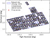 |
Fig. 1. COSMOS2020 sources observed by the COSMOS-Web program. Blue rectangles indicate the tiles reduced by Zhuang et al. (2024). Red squares are the X-ray sources identified by Marchesi et al. (2016). |
2.3. X-ray, far-IR, and sub-millimetre data
We included X-ray photometry from the Chandra COSMOS Legacy survey (Civano et al. 2016; Marchesi et al. 2016). We selected X-ray sources from the catalogue of optical and IR counterparts presented by Marchesi et al. (2016) that have a final counterpart identification Flag = 1 (secure) or = 10 (ambiguous), and a star flag Star ≠ 1, 10, 100 (which identify stars spectroscopically, photometrically, and visually, respectively). We then cross-matched this catalogue with our selected sources in COSMOS2020 within a radius of 1″ of the optical coordinates. We found a total of 270 cross-matched X-ray sources. The Marchesi et al. (2016) catalogue provides only upper limits for some sources. Nevertheless, we kept these sources since the SED fitting tool employed can deal with upper limits.
The following far-IR and sub-millimetre (sub-mm) data are available in the COSMOS field: i)Spitzer/MIPS 24 μm data provided by the COSMOS-Spitzer programme (Sanders et al. 2007); ii)Herschel/PACS maps from the PACS Evolutionary Probe (PEP; Lutz et al. 2011) survey; iii)Herschel/SPIRE maps from the Herschel Multi-tiered Extragalactic Survey (HerMES; Oliver et al. 2012). Wang et al. (2024) deblended these far-IR and sub-mm maps with a novel progressive and probabilistic approach. In this way, the multi-wavelength information, the full posterior, the variance, and the covariance between sources are exploited. In this paper, we used the deblended catalogue released by Wang et al. (2024) to add the far-IR and sub-mm data. Wang et al. (2024) constructed their initial prior catalogue from the COSMOS2020 catalogue. Therefore, we used the galaxy’s unique IDs to cross-match the sources. We found 13 924, 4392, and 1741 MIPS, PACS, and SPIRE counterparts, respectively. For galaxies with a measured far-IR flux below the corresponding total noise (instrumental plus confusion noise), we set the total noise to be the flux upper limit (see Table 3 in Wang et al. 2024).
3. Methods
In this section, we first describe the SED fitting method we employed, and then our AGN selections. In the second part, we discuss the deep learning algorithm and the mock galaxy images used to identify mergers.
3.1. CIGALE SED fitting
We estimated galaxy physical properties using the SED fitting tool Code Investigating GALaxy Emission (CIGALE; Burgarella et al. 2005; Noll et al. 2009; Boquien et al. 2019). The 2022.1 version3 includes AGN models and can exploit data from X-ray to radio wavelengths (Yang et al. 2020, 2022). The complete parameter space of the CIGALE configuration used is provided in Appendix A, Table A.1. Here, we briefly describe the CIGALE configuration. We employed a delayed−τ plus an optional exponential starburst star-formation history, which can model both early- and late-type galaxies, using small and large τ, respectively (Boquien et al. 2019). Moreover, including an optional exponential burst component can account for potential recent star formation. We utilised the Bruzual & Charlot (2003) single stellar population model, with Chabrier initial mass function (IMF) and solar metallicity; the modified Charlot & Fall (2000) as a dust attenuation law; and the Draine et al. (2014) models as dust emission templates.
We used the SKIRTOR model for the AGN component (Stalevski et al. 2012). SKIRTOR assumes a flared disc geometry for the dust distribution and models the dusty torus as a two-phase medium consisting of high-density clumps and a low-density medium which fills the space between the clumps in the 3D structure. We set CIGALE to measure the AGN fraction, fAGN, defined as the AGN contribution to total galaxy emission, in the rest-frame wavelength range 3 − 30 μm. We included the X-ray module Yang et al. (2020, 2022) for modelling X-ray emission from both AGN and galaxies (due to hot gas and X-ray binaries). When only upper limits are available, these values are passed on to CIGALE as such.
Figure 2 shows the stellar mass distribution of the sample as a function of z. We selected a stellar-mass complete sample (for both quiescent and star-forming galaxies) using the KS-based completeness function from Weaver et al. (2022) for the COSMOS2020 sample. As we train our DL models on galaxies more massive than 109 M⊙, it is reasonable to set this as a lower mass limit. Therefore, we select galaxies with M★ higher than the maximum of 109 M⊙ and the KS-based completeness limit. In addition, our sample is limited to galaxies with reliable SED fits (i.e. reduced χ2 < 5). After applying cuts on mass and χ2, we obtained 22 862 galaxies, excluding 2310 located at the edges of the JWST tiles. The final mass-complete sample consists of 20 552 galaxies between z = 0.5 and 2. The median CIGALE error is σ(log10 M★) = 0.1 for stellar mass, σ(log10SFR) = 0.2 for SFR, and σ(fAGN) = 0.1 for AGN fraction. We further assess the reliability of galaxy property measurements in Appendix A, with example best-fit SEDs.
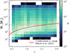 |
Fig. 2. Stellar mass vs redshift. The red line represents the KS-based completeness for the COSMOS2020 sample (Weaver et al. 2022). The dashed line indicates the simulations’ lower mass limit (M★ = 109 M⊙). |
Additionally, we ran CIGALE without SKIRTOR and X-ray modules, keeping all other parameters as in Table A.1. This test was meant to check whether galaxies could be fitted equivalently well without an AGN component. The output results helped identify a purer and more reliable sample of SED AGN, as described in the next subsection.
3.2. AGN selections
We selected AGN in three different ways. First, following Marchesi et al. (2016), we selected 104 secure X-ray AGN by requiring DET_ML (the maximum likelihood detection) > 10.8 in the hard or soft band. In about half of the cases (49/104) DET_ML is > 10.8 in both bands. In Fig. 3, we show the X-ray luminosity as a function of redshift, in both soft and hard bands, for the selected X-ray AGN. No sources in the hard band have luminosities LX < 1042 erg s−1, which is the threshold conventionally used to identify clear AGN from galaxies (Rosario et al. 2012). In the soft band, roughly 7% of the sources have 1041 < LX < 1042 erg s−1. However, excluding these sources does not affect our results, so we keep them in the sample.
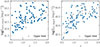 |
Fig. 3. Rest-frame soft (left) and hard (right) X-ray luminosities vs redshift for the selected X-ray AGN. Black arrows are upper limits. |
Second, we identify AGN by their MIR emission in galaxies with Spitzer/MIPS 24 μm flux F24 μm > 20 μJy, which is the 1σ total noise (instrument plus confusion noise). Then, we required S/N > 5 in each IRAC channel and applied the colour–colour criteria in Chang et al. (2017)4
 (1)
(1)
 (2)
(2)
 (3)
(3)
 (4)
(4)
where x = m3.6 μm − m5.8 μm and y = m4.5 μm − m8 μm. Magnitudes are in the AB system. This colour–colour selection is displayed in Fig. 4, left panel. In total, we found 159 MIR AGN. We show their rest-frame 6 μm luminosity in the right panel of Fig. 4.
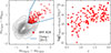 |
Fig. 4. Left: IRAC colour–colour space. Red crosses are the selected MIR AGN. Contours show the population satisfying the 24 μm flux and S/N requirements. The blue box indicates the Chang et al. (2017) selection. Right: Rest-frame 6 μm luminosity of the AGN component vs redshift for the selected MIR AGN. |
Third, we defined SED AGN as those galaxies where the inclusion of an AGN component significantly improves the fit to the observed photometry. To assess the necessity of the AGN component, we compared the CIGALE runs that include the AGN module with the run that excludes the AGN module. We classified a source as an SED AGN only if the relative improvement in the reduced χ2 exceeded 10% or the fit without the AGN component failed. Furthermore, to ensure that AGN identification is physically constrained by the hot dust emission rather than fitting degeneracies in the rest-frame near-infrared, we imposed a strict MIR photometric requirement: a detection with S/N > 5 in all four Spitzer/IRAC channels (3.6, 4.5, 5.8, and 8.0 μm). Finally, we required an AGN fraction fAGN > 0.2. This threshold exceeds the typical CIGALE median uncertainty of 0.1, minimising misclassifications, while the combination of the χ2 evaluation and MIR coverage criteria ensures the presence of a robust MIR excess due to the presence of an AGN.
In summary, SED AGN respect the following three criteria
 (5)
(5)
 (6)
(6)
 (7)
(7)
We found 1334 SED AGN in our sample. Figure 5 summarises the numbers and overlaps between the categories in our sample. Although our SED AGN incorporate most of the MIR and X-ray AGN (≈80%), these two diagnostics still identify unique AGN that are missed by the SED definition.
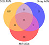 |
Fig. 5. Venn diagram of the three AGN types. |
We show the AGN luminosity distribution for the three classes in Fig. 6. As a proxy for the bolometric luminosity, we used Ldisc, the ‘accretion power’ parameter of CIGALE, which is equivalent to the angle-averaged AGN bolometric luminosity (Yang et al. 2018). In general, MIR and X-ray AGN exhibit intermediate-to-high Ldisc, with the MIR AGN constituting the brightest sample on average. Conversely, the SED AGN selection extends to a larger population of faint sources, particularly at z > 1.2, although the majority of this sample still shows intermediate luminosities. We show the fAGN distributions for the three AGN selections and the entire galaxy sample in Fig. 7. The galaxy population peaks at low fAGN values (mostly < 0.20) and monotonically decreases with increasing fAGN. The SED AGN follow this trend, but starting at fAGN ≥ 0.20. The MIR and X-ray AGN show different distributions. The MIR AGN distribution is roughly flat, with a slight skew towards high fAGN values. This is expected as we measure fAGN in the rest-frame 3 − 30 μm range. The X-ray distribution is also broadly uniform, with a peak at fAGN ≈ 0.2 − 0.3.
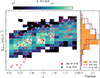 |
Fig. 6. AGN disc accretion luminosity as a function of redshift, for MIR (red crosses), X-ray (blue circles), and SED AGN (2D histogram). On the right margin, we display the Ldisc histogram distributions for the three AGN selections. |
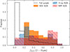 |
Fig. 7. Normalised AGN fraction distribution for the three AGN classes (SED: orange bars; X-ray: blue bars with vertical stripes; MIR: red bars with diagonal stripes) and the entire galaxy sample (dashed black line). |
3.3. Merger identification
We used convolutional neural networks (CNNs) trained on realistic mock images of simulated galaxies as our merger classifier. We employed two different simulations for this task. The IllustrisTNG cosmological hydrodynamical simulation consists of three different volumes varying in physical size and mass resolution (Marinacci et al. 2018; Naiman et al. 2018; Nelson et al. 2018; Pillepich et al. 2018; Springel et al. 2018). We used the highest resolution version of the TNG-100 box (hereafter referred to as TNG), whose side corresponds to ≈110.7 Mpc and has a baryonic matter resolution of 1.4 × 10⁶ M⊙. This mass resolution allowed us to select galaxies down to M★ = 109 M⊙. Galaxies were selected in the range z = 0.5–2 (corresponding to snapshot numbers 67 − 33). For each galaxy identified through the Subfind algorithm (Springel et al. 2001), TNG provides a complete merger history (Rodriguez-Gomez et al. 2015).
Horizon-AGN is a cosmological hydrodynamical simulation of a 100 Mpc3 h−1 comoving volume. It has a stellar mass particle resolution of 2 × 10⁶ M⊙ (Dubois et al. 2014), comparable to that of TNG-100. We identified galaxies with the AdaptaHOP algorithm, updated to construct merger trees (Tweed et al. 2009). In this case, galaxies were also selected in the z = 0.5–2 range and with M★ > 109 M⊙. For both simulations, we observed each object from three different projections.
3.3.1. Generation of mock galaxy images
We defined as mergers those galaxies that had a major merger (with a stellar mass ratio ≤4) in the last 300 Myr and/or will coalesce in the next 800 Myr. Galaxies not meeting these criteria were labelled as non-mergers. We found 45 850 and 42 630 mergers in TNG and Horizon-AGN, respectively. We selected the same number of non-mergers in both simulations, roughly matching the stellar mass and redshift distributions of mergers. We created mock F150W observations of simulated galaxies from three different points of view. To obtain reliable classifiers, it is crucial to include observational effects (Huertas-Company et al. 2019; Rodriguez-Gomez et al. 2019). We generated synthetic observations following Margalef-Bentabol et al. (2024a):
-
We created galaxy thumbnails with a physical size of 50 kpc × 50 kpc and the same pixel resolution as the real NIRCam images (0.03″/pixel). Each stellar particle contributes to the galaxy’s SED, determined by its mass, age, and metallicity. We derived these SEDs from the stellar population synthesis models of Bruzual & Charlot (2003). The integrated SED was passed through the F150W filter to generate a smoothed 2D projected map (Rodriguez-Gomez et al. 2019).
-
We convolved each image with the filter point spread function (PSF), randomly choosing one from the 80 PSF models derived by Zhuang et al. (2024). We then added Poisson noise to the convolved images as shot noise.
-
To make observations as realistic as possible, each mock observation was injected into real F150W sky cutouts. We created F150W cutouts that do not contain any bright source at the centre and without artefacts but still allow for possible background galaxies and faint sources. We generated random coordinates within the covered area and ensured that there were no z < 3 sources in COSMOS2020 within a radius of
 . This radius was derived from the estimated source density of COSMOS2020. The generated coordinates were used as the centres of our cutouts, which were 320 pixels across (corresponding to ∼ 60 kpc at z = 0.5). To ensure that no stellar spikes are present in the cutouts, we ran Kendall’s τ test (Kendall 1938) along both image axes. If a strong correlation among pixels was found, that is, a p-value < 0.001, the cutout was rejected5. For each mock galaxy, we randomly picked a sky cutout and injected the galaxy into its centre.
Although we previously explored incorporating dust via radiative transfer, we found the computational cost to be extremely high, while the impact on the resulting morphologies–and on classification performance–was minimal (Bottrell et al. 2019; Rodriguez-Gomez et al. 2019; Wang et al. 2020). Therefore, we opted to use dust-free simulations in this work.
To account for potentially bright AGN, we included a central point source in 20% of the simulated galaxies (randomly selected), using the PSF models derived by Zhuang et al. (2024). As performed by Margalef-Bentabol et al. (2026), the PSF contribution fraction (with values drawn uniformly between 0 and 1) was defined in relation to the host galaxy
 (8)
(8)
where FPSF and Fhost are the fluxes within a  aperture of the central source and the host galaxy, respectively.
Our CNN takes as input images of the same size. Thus, we resized all images to a common size of 256 pixels across, corresponding to ∼ 50 kpc at z = 0.5. Following Bottrell et al. (2019), all images were hyperbolic arcsin-scaled in the range 0–1, and the contrast of the central target was maximised as follows:
-
We took the hyperbolic arcsin of the sky-subtracted images. Values below −7 were converted to NaNs.
-
We computed the median of each image, amin, and the 99th percentile, amax, considering a central box of side 80 pixels.
-
All values < amin were set to amin, including NaNs. Values > amax were set to amax. Then, the clipped images were normalised by subtracting amin and dividing by amax − amin.
3.3.2. CNN training
We developed a CNN to classify galaxies into mergers and non-mergers, utilising the Keras framework for the TensorFlow platform (Chollet 2023; Abadi et al. 2016) for the architecture implementation. The CNN consists of four convolutional layers and three fully connected layers. The output map of each layer is passed to the next layer. For all layers, we adopted a rectified linear unit as an activation function. A stride of one pixel was used for the convolutional layers. We introduced dropout layers after each processing layer to prevent over-fitting. These dropout layers randomly set the input units to 0 at a rate specified by the user. To further prevent over-fitting, early stopping in the training phase was used. The architecture and specific hyper-parameters are reported in Appendix B, Table B.1.
We trained an identical CNN using mock galaxy observations from both the TNG and Horizon-AGN simulations. We designate the CNN trained on TNG images as TNG-CNN and the one trained on the Horizon-AGN dataset as HA-CNN. The CNN output is a score for each input image, in turn, used to make the classification. We split each mock galaxy sample into train, validation, and test sets, using a 80–10–10 split. We initially evaluated each model performance on its associated test set using common metrics such as ‘precision’, ‘recall’, and ‘F1-score’ calculated for the merger class. TNG-CNN has a precision of 0.74, a recall of 0.61, and an F1-score of 0.67 on the TNG test set. Overall, HA-CNN shows better performance with a precision of 0.76, recall of 0.69, and F1-score of 0.72.
3.3.3. Predicting on JWST/F150W images
To reliably distinguish morphological features, we restricted the sample to those with S/N > 10. We calculated S/N by performing aperture photometry with a circular aperture centred on each galaxy, with a radius of 2.5 kpc in the galaxy z. The background noise is calculated using 500 blank cutouts. In each blank cutout, we applied sigma clipping (σ = 3.0) and calculated the root mean square. Then, we computed the median background noise of the 500 cutouts. We found 13 789 galaxies with S/N > 10 in the range z ∈ [0.5; 2.0]. This is the sample of galaxies on which we focus in this paper.
We evaluated the performance of the models using a test set of real JWST/F150W images. For this task, three of us (ALM, LW, BMB) visually inspected 2000 galaxies, randomly sampled in the range 0.5 ≤ z ≤ 2. A galaxy was labelled as a merger or non-merger only if all three classifiers agreed on the class; otherwise, the galaxy was rejected. The identification of mergers was based on the presence of a companion of comparable size, morphological disturbances such as tidal tails or bridges, and highly irregular structures indicative of recent or ongoing interactions.
The final, visually inspected sample contained 891 non-mergers and 378 mergers and was used to measure the performance of the CNNs on the real observations. This test set was balanced to obtain an even number of mergers and non-mergers, randomly sampling 378 non-mergers among the 891 available. This step was repeated multiple times, but the final results did not change. For both models, we searched for the best threshold to divide mergers and non-mergers, defined as the threshold that maximises the F1 score, maintaining a precision > 0.80 for the merger class. The results are reported in Table 2. Overall, the two models show similar good performance in the visually inspected test set, with precision of ≃0.8 and recall of ≃0.7 for the merger class.
Overall CNN performance on the visual test set.
3.3.4. The combined CNN classifier
We followed LM24 to have even higher classification precision by combining the TNG-CNN and the HA-CNN into a single classifier (hereafter Comb-CNN). Comb-CNN works as a logic AND operator, as shown in Fig. 8: if both CNNs agreed on the class (merger or non-merger), then the image was classified as such; otherwise, it was labelled as ’unclassified’. We searched for the best thresholds using a similar approach as for the individual models. We looked for the combination of two thresholds (TTNG and THA) that gives the best F1 score, with the constraint of a merger class precision > 0.8. Additionally, as Comb-CNN excludes some galaxies, we ensured at every step that the test set contained at least 250 visually classified mergers and 250 non-mergers. For each threshold combination, the test set was re-balanced 20 times, and the metrics were calculated as the median value of the 20 drawings. Each threshold was varied in the range of 0.3–1.0, with a step of 0.01. As the best combination of thresholds, we found TTNG = 0.50 and THA = 0.56. The performance of Comb-CNN with these thresholds is reported in Table 2. Comb-CNN performs better than individual models, having a merger-class precision of 0.88 and a recall of 0.90. We show the confusion matrix of Comb-CNN with the best threshold combination in Fig. 9.
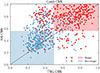 |
Fig. 8. Comb-CNN classification for the visually inspected test set (mergers: red circles; non-mergers: blue crosses). The scores predicted by the TNG-CNN and the HA-CNN are reported on the x- and y-axes, respectively. The shaded red or blue area defines the region of galaxies classified as mergers or non-mergers by the Comb-CNN. Sources in the white areas are labelled as unclassified. |
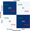 |
Fig. 9. Comb-CNN confusion matrix for the visually inspected test set. Each cell shows the number of objects at its centre, the fraction of objects normalised by column (green percentages) in the top left corner, and the fraction of objects normalised by row (red percentages) in the lower right corner. On the main diagonal, these percentages correspond to precision and recall, respectively. |
We used Comb-CNN and the best thresholds to classify all selected galaxies. Of the initial 13 789 galaxies, 8285 have been classified as mergers (2276) or as non-mergers (6009), while 5504 have been labelled as unclassified. Hereafter, we focus on the sample of classified galaxies. In Appendix C, we show some examples of galaxies identified as mergers and as non-mergers by our classifier.
4. Results
In this section, we present the properties of the AGN host galaxies, demonstrating the importance of constructing proper control samples. Then, we analyse the merger–AGN relation adopting a simple binary AGN or non-AGN classification and a continuous approach, exploring the relative and absolute AGN power.
4.1. The host galaxies of AGN and non-AGN
We defined non-AGN galaxies as those not identified as X-ray or MIR AGN and with fAGN < 10%. In Fig. 10, we show the SFR–M★ plane and the M★ distributions for the three types of AGN and the non-AGN. The X-ray AGN inhabit intermediate and high-mass galaxies, with a median value of 1010.9 M⊙. Many X-ray AGN are below the MS, appearing to be transitioning towards quiescence (the ‘green valley’). The MIR AGN tend to be hosted by intermediate-mass galaxies (with a median M★ of 1010.3 M⊙) on the MS, with the lowest fraction of quenched galaxies. The host galaxies of SED AGN exhibit a M* distribution comparable to that of MIR AGN (median M★ of 1010.3 M⊙), and generally follow the MS, while showing a secondary overdensity in the quenched and red-sequence region. In comparison, non-AGN have larger fractions of low-mass galaxies (with a median value ∼109.9 M⊙), and display both a star-forming MS and a passive red sequence. In Appendix D, we further investigate the SFR–M★ relation as a function of the AGN luminosity and for exclusive types of AGN.
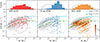 |
Fig. 10. SFR vs M★ for the three AGN types. We show the SED AGN as a 2D distribution. In each panel, the contours (from 10% to 90%, with intervals of 10%) represent the non-AGN distribution. The dashed blue and the dash-dotted green lines indicate the MS at z = 2 and z = 0.5 from Popesso et al. (2023), respectively. On top of each panel is the M★ distribution of the AGN and the corresponding non-AGN (grey). |
Our stellar mass distributions of the AGN host galaxies agree with previous results. Bongiorno et al. (2012) showed that the mass distribution of the previous generation of X-ray AGN in COSMOS peaks at 1010.9 M⊙. Mountrichas et al. (2022) selected X-ray AGN using the eROSITA Final Equatorial-Depth Survey (eFEDS) and found a median host M★ of 1011 M⊙. On selecting X-ray AGN from the XMM-XXL survey, Mountrichas et al. (2021) found an average host M★ ≃ 1010.9 M⊙ for type I AGN and M★ ≃ 1010.6 M⊙ for type II AGN. Similarly, Rosario et al. (2013) found that the peak in the AGN host galaxy mass distribution is at 1010.5 − 10.7 M⊙. Bornancini et al. (2022) and Azadi et al. (2017) observed a host mass distribution for MIR AGN comparable to the one we present, with a median value at 1010.5 M⊙. In a recent study of optically selected Type II AGN, Vietri et al. (2022) found that the stellar masses of AGN hosts have a median value of 109.5 M⊙, slightly lower than what we observe for the MIR and SED AGN.
The location of the X-ray AGN in the SFR–M★ plane agrees with what Cristello et al. (2024) observed. Similarly, Bongiorno et al. (2012) and Azadi et al. (2015) found that X-ray AGN often inhabit massive red galaxies. Mullaney et al. (2015) and Silverman et al. (2008) found that the host galaxies of X-ray AGN are on average below the MS. Previous studies also uncovered a SFR dependence on X-ray luminosity LX, with SFRs lower or comparable to those of star-forming galaxies at LX < 1044 erg s−1, and slightly enhanced SFRs at higher LX (Rosario et al. 2012; Santini et al. 2012; Mountrichas et al. 2021, 2022). These results seem to be in contrast to our Fig. 10. However, Mountrichas et al. (2021, 2022) excluded quiescent systems. Rosario et al. (2012) derived mean SFRs through stacking, which can be biased towards the star-forming population compared to the median distribution, while Santini et al. (2012) considered only galaxies detected in the far-IR. Ellison et al. (2016) found that MIR AGN have, on average, enhanced SFRs compared to non-active galaxies and are frequently hosted by massive star-forming galaxies, in agreement with our results. Azadi et al. (2017) also reported that IR-selected AGN lie on or above the MS. For AGN identified with optical spectroscopy, Vietri et al. (2022) found a broader distribution of SFRs than the MS, similar to that of non-AGN galaxies: massive galaxies have a larger fraction of quenched galaxies, while lower mass galaxies are on the MS. This picture is consistent with our SFR–M★ distribution for the SED AGN, which is most similar to that of non-AGN. Our results and previous findings underscore an important caveat in AGN selection: host galaxies of different AGN types systematically differ from each other. Thus, it is important to have control galaxies that match the AGN sample in stellar mass, redshift, and SFR.
4.2. Control samples
We compared the merger and the AGN populations to control samples of non-mergers or non-AGN, respectively. Specifically, the controls satisfied the following conditions
 (9)
(9)
 (10)
(10)
 (11)
(11)
where Δz = 0.03, ΔlogM★ = 0.1 dex, and ΔlogSFR = 0.3 dex. We chose these values based on the photo-z precision and the median errors for M★ and SFR. For each galaxy in the original sample, we required at least ten counterparts that satisfied these criteria. We randomly picked ten if more than ten controls were found. If there were fewer than ten controls, we iteratively increased the tolerance of each parameter by a factor of 1.5. This operation was performed up to a maximum of three times; otherwise, we rejected the galaxy. For non-AGN controls, we only considered galaxies that do not host any detected AGN.
To make a fair comparison with the results presented in LM24, we built control samples without matching SFRs and ran our experiments with these controls. However, the results were qualitatively the same, with all variations within 1σ uncertainties. Therefore, we did not report the results of this test.
4.3. Merger–AGN relation using a binary AGN classification
In the first set of experiments, we investigate the merger–AGN connection with a binary AGN or non-AGN classification. If mergers trigger AGN, we would expect a higher incidence of AGN in mergers than in non-merger controls. If mergers are the primary trigger, we should observe that most AGN are in mergers. We divided the sample into two redshift bins, z-bin 1 =[0.5; 1.25) and z-bin 2 =[1.25; 2.0], with roughly equal numbers of AGN.
4.3.1. AGN frequency in mergers and non-mergers
We show the frequency of AGN in mergers and non-merger controls in Fig. 11 and report the exact values in Appendix E, Table E.1. For all types of AGN and z-bins, we observe a marginally higher frequency of AGN in mergers, demonstrating that mergers are a viable way to fuel accretion onto SMBHs. We also calculated the AGN excess by taking the ratio of the AGN frequency in mergers relative to non-mergers. About 1.5% and 4% of mergers host MIR AGN in z-bins 1 and 2, respectively, compared to ∼1% and 3% in non-mergers. Hence, the MIR AGN excess is 1.3 − 1.4 in mergers, which is significant at 2σ level in z-bin 2 but is compatible with no excess in z-bin 1. Roughly 2% of the mergers host X-ray AGN in both z-bins, compared to < 1% in non-mergers. This leads to an X-ray AGN excess ratio of 2.6 in mergers (significant at ∼2.5σ), which is the highest among the three types of AGN. Around 14% and 22% of mergers host SED AGN in z-bins 1 and 2, respectively, compared to ∼12% and ∼18% in non-mergers. Consequently, the SED AGN excess is the lowest among the three types. The excess is almost negligible in z-bin 1 (1.10 ± 0.09), and modest (1.20 ± 0.07), although significant at ∼3σ, in z-bin 2.
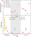 |
Fig. 11. Top: Frequency of AGN (MIR: red; X-ray: blue; SED: orange) in mergers, indicated with filled symbols, and non-merger controls, empty symbols. Bottom: AGN frequency in mergers divided by the AGN frequency in the relative non-mergers (i.e. AGN excess). |
Recent studies in z < 1 found higher MIR AGN excesses in mergers than what we observe (excesses ≃1.5–7; Goulding et al. 2018; Bickley et al. 2023; La Marca et al. 2024). Our X-ray AGN excess is in line with the results in Lackner et al. (2014). On the other hand, the X-ray AGN excess we find is larger than what was observed at lower redshift by Bickley et al. (2023, excess ≃1.8) and LM24, excess ≃1.9, but still within the 1σ uncertainty. Our results for SED AGN are slightly lower but still in agreement with previous studies of SED AGN (LM24) and of AGN selected with optical-emission-lines (Gao et al. 2020; Tanaka et al. 2023). Fewer studies investigated AGN frequency in mergers and non-mergers at z > 1. Our results are qualitatively in agreement with Silva et al. (2021), who observed a mild excess of AGN in mergers that decreases as a function of redshift. This experiment shows that mergers can trigger AGN, but it is unclear if there is a strong dependence on the redshift. There is some expectation (Kocevski et al. 2015) that mergers may play a less important role at intermediate and high redshifts and, consequently, the greater role that secular processes play in feeding SMBHs, due to the greater availability of cold gas (Tacconi et al. 2010).
4.3.2. Merger fraction in AGN and non-AGN
We report the merger fraction (fmerg) in AGN and non-AGN controls in Fig. 12 and Table E.2. For all z-bins and AGN types, fmerg is higher in AGN than in non-AGN controls, strengthening the merger–AGN connection. About half of the X-ray AGN in both z-bins are hosted by mergers (48% and 56%), while fmerg is 22% and 28% in the corresponding non-AGN controls. The MIR AGN are hosted by mergers in 27% (48%) of the cases in z-bin 1 (z-bin 2), while 18% (36%) of the non-MIR AGN controls are mergers. For SED AGN, fmerg is around 23% (40%) in z-bin 1 (z-bin 2), while fmerg is around 17% (34%) in the non-SED AGN controls. The merger fractions are larger in the second z-bin for all types of AGN, in agreement with the previously observed rising fmerg with increasing z (Ferreira et al. 2020).
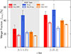 |
Fig. 12. Merger fraction in the AGN (filled bars) and non-AGN controls (empty bars), with the same colour coding as Fig. 11. |
Overall, we report only a slight enhancement in fmerg in AGN compared to non-AGN controls. fmerg is ∼50% only for the X-ray AGN in both z-bins and MIR AGN in z-bin 2, indicating that mergers might be the main triggering mechanism or at least play an important role in these cases. However, we also observe significant merger fractions in non-AGN controls. Hence, AGN could be ubiquitous in mergers and non-mergers but episodic. We should consider a scenario in which not all mergers trigger the AGN phase. In this case, the difference between fmerg in AGN and fmerg in non-AGN represents the real fraction of mergers that trigger AGN. For example, considering MIR AGN in z-bin 2, only 48%−36% = 12% of all MIR AGN are triggered solely by mergers. In a different case, it might be possible that all mergers trigger AGN, but the AGN happen to be ‘off’ in some galaxies, given the mismatch in the merger and AGN timescales. This scenario would imply that 48%+36% = 84% of MIR AGN are triggered by mergers.
Our results are qualitatively in agreement with previous studies. Mechtley et al. (2016) studied a sample of quasars up to z = 2 and observed a marginally larger fmerg in quasar hosts than in inactive galaxies. Similarly, Marian et al. (2019) and Kocevski et al. (2012) found only slightly larger fmerg in the X-ray AGN compared to inactive control galaxies. Villforth (2023) conducted a review and concluded that in most cases, fmerg in AGN is consistent with no excess over controls. Nevertheless, other studies reported higher fmerg. Fan et al. (2016) found that the most luminous dust-obscured AGN are more likely to be classified as disturbed, with a high fmerg (62%). With a larger sample including faint sources, Bonaventura et al. (2025) observed that a high fraction of AGN hosts are strongly disturbed. Similarly, Donley et al. (2018) found that more than 70% of MIR AGN are classified as interacting or highly disturbed. However, these studies are biased towards bright and heavily obscured objects, which are more supported observationally as being connected with major mergers (Ricci et al. 2017, 2021).
4.4. The merger link with AGN relative and absolute power
We now examine the merger–AGN connection using a continuous approach. We make use of the relative and absolute AGN power, traced by the AGN fraction (fAGN) and the AGN accretion disc luminosity (Ldisc), respectively.
4.4.1. The merger fraction and AGN fraction relation
We display the fAGN distribution for mergers and non-merger controls in Fig. 13. The MIR AGN show large fractions of host galaxies with fAGN > 0.7 for both mergers and non-mergers. This is expected because fAGN is measured in the 3 − 30 μm range, and the MIR diagnostics preferentially trace obscured AGN. However, mergers harbouring MIR AGN show a larger fraction at fAGN > 0.7 compared to non-mergers. For the X-ray AGN, the fAGN distributions appear to be bimodal, with peaks at 0.3 and 0.8 for both mergers and non-mergers. Non-mergers have larger fractions of galaxies with fAGN ≤ 0.3 than mergers. Finally, the fAGN distributions for the SED AGN do not show a significant difference between mergers and non-mergers, only a slightly larger fraction of mergers at fAGN ≥ 0.8. We ran two-sample Kolmogorov-Smirnov (KS; Hodges 1958) tests to measure the statistical difference between the distributions in mergers and non-mergers (reported in Fig. 13), which confirm that the mild differences are not statistically significant.
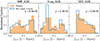 |
Fig. 13. AGN fraction normalised distributions for mergers (orange) and non-merger controls (empty blue bars), divided by AGN type. In each panel, we display the results of the KS-test run for the two populations. |
We present the fmerg–fAGN relationship for the three AGN types in Fig. 14. We computed fmerg in N bins (with N randomly sampled between 6 and 20) of fAGN, equally spaced in the range 0–1. The trends reported represent the running medians of 1000 bootstrap samples for each population. The MIR and SED AGN show a rather flat fmerg in the range fAGN = 0.1–0.6. At fAGN > 0.6, MIR AGN have an increase in fmerg while SED AGN have a more gentle increase in fmerg. X-ray AGN show a more complicated trend: a slightly increasing fmerg until fAGN = 0.6, followed by a mild decrease in fmerg in the range fAGN = 0.6–0.8, in turn followed by an increase fmerg at fAGN > 0.8. Moreover, half of the X-ray AGN inhabit mergers. Based on these results, we conclude that mergers could be the main triggering mechanisms for the most dominant MIR and X-ray AGN (fAGN > 0.8).
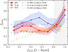 |
Fig. 14. Merger fraction as a function of AGN fraction for the MIR AGN (red crosses), X-ray AGN (blue circles), and SED AGN (orange triangles). The solid lines and coloured region show the running median and standard deviation of each relation. The dashed lines indicate the fits to the relations in LM24. The light grey area indicates the region where the relationships’ behaviours change strongly (see text). |
We compare the fmerg–fAGN relation with the same relation in LM24 at z < 0.8. The low-redshift relation revealed two different regimes for all types of AGN: a flat fmerg to fAGN < 0.8 and a subsequent steep rise in fmerg at fAGN > 0.8. To compare with the relation in COSMOS-Web, we parametrised the LM24 fmerg–fAGN relation, with details on the fitting method and results in Appendix F. In Fig. 14, we report the fitted relations by AGN type. Considering the fAGN < 0.8 regime, there is a qualitatively good agreement between our results and LM24, with a slight difference. The plateau level for each AGN selection is slightly different at low and high redshifts. Taking into account the same SED AGN definition adopted here (fAGN > 0.2), SED AGN have on average the same fmerg plateau value shown in LM24 but show a flatter trend. The MIR AGN show a larger merger fraction at z < 0.8 than at 0.5 < z < 2, possibly due to the different luminosity ranges covered. The contrary is true for the X-ray AGN, which are hosted more frequently by mergers at higher redshifts. Nevertheless, given the large uncertainties, our findings are consistent with no significant differences from the trend reported in LM24. Although similar in the low-dominance AGN regime, more differences emerge at fAGN > 0.8. MIR, X-ray, and SED AGN show a steeper rise at low redshift compared to high redshift. This is most evident for the SED AGN, where there is only a slight increase for the 0.5 < z < 2 galaxies.
Two aspects require further discussion. First, the reason why SED AGN do not show a steep increase fmerg for dominant AGN may be because SED AGN are usually fainter than MIR and X-ray AGN. Even relatively dominant SED AGN with fAGN > 0.8 might still be faint in absolute terms. Lower luminosities correspond to lower SMBH accretion rates, which secular processes could sustain if enough gas is available. Second, fmerg shows a steeper rise for dominant MIR and X-ray AGN at low z than at high z, hinting at a lower importance of mergers in triggering dominant AGN at cosmic noon than at lower redshifts. This may be possible, given the different gas supplies available. At higher z, galaxies have larger gas fractions and stochastic fuelling by internal processes could play a greater role than at lower z (Kocevski et al. 2012, 2015). At z < 1, galaxies generally have lower gas fractions, and so external sources are necessary to enlarge the gas content and fuel dominant AGN (Tang et al. 2025).
Nevertheless, it is worth noting that the availability of gas alone is not sufficient to trigger SMBH accretion. Efficient accretion also requires the removal of angular momentum, which can be achieved not only via major mergers but also by bars or secular instabilities, particularly in gas-rich discs (Combes 2001). Hence, a key difference might be that mergers at low-z are necessary not only to remove the angular momentum but also to bring in new cold gas to fuel nuclear activity. Thus, it is likely that the role of mergers, as a function of fAGN, evolves with cosmic time (and/or gas content): mergers gain importance in fuelling dominant AGN with decreasing z (or gas content), becoming the sole viable mechanism to feed the most dominant AGN at z = 0.
4.4.2. The merger fraction and Ldisc relation
Now we analyse the merger–AGN connection using the absolute AGN power. We show the normalised Ldisc distribution for mergers and non-merger controls in Fig. 15. Overall, the merger and non-merger distributions are similar for all AGN types, although in the case of SED AGN, mergers show larger fractions of bright AGN (Ldisc) compared to non-merger controls, as confirmed by the KS-test results. It is worth mentioning that, looking at the very bright end (Ldisc ≳ 1046 erg s−1), there is an excess in the fraction of mergers compared to the fraction of non-mergers also for MIR and X-ray AGN.
We plot the fmerg–Ldisc relation in Fig. 16, in the same way as for the fmerg–fAGN relation, with the only difference being the NLdisc bins evenly spaced on a logarithmic scale. For all three types of AGN, fmerg rises as a function of increasing Ldisc, with mergers accounting only for ≲20% of the faint AGN (Ldisc ≲ 1043 erg s−1) but being the dominant trigger of the brightest AGN (Ldisc ≳ 1046 erg s−1). These results imply that the role of mergers is directly linked to the absolute power of the AGN, with mergers being the most efficient process to fuel the most powerful AGN. We could also interpret these results from another angle, i.e., secular processes become less efficient in fuelling AGN activity above a certain threshold.
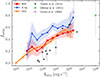 |
Fig. 16. Merger fraction–AGN luminosity relation for the three AGN types. The solid line and coloured region show the running median and standard deviation of each relation. Previous literature findings are reported. |
These findings align with most previous results in the literature. The early work of Urrutia et al. (2008) analysed a limited sample of bright quasars and found that > 80% of them exhibit clear signs of recent or ongoing major interactions. Similarly, Glikman et al. (2015) observed an fmerg of 80% for a sample of extremely bright quasars. Treister et al. (2012), Donley et al. (2018) and Euclid Collaboration: La Marca et al. (2026) also reported an increase in fmerg as a function of AGN luminosity, with mergers becoming the dominant mechanism for LAGN > 1045.5 erg s−1. However, other studies did not find a clear correlation between fmerg and AGN luminosity. For example, our results are at odds with those reported by Allevato et al. (2011), Hewlett et al. (2017), and Villforth (2023), which found no evidence to support the scenario in which the most luminous AGN reside mainly in mergers. However, the reasons for this conflict remain unclear. This may be due to the small sample sizes and/or the different selections of those studies, which makes a fair comparison difficult.
A further impediment in studying the merger–AGN connection is the timescales. While the AGN duty cycle usually lasts 10 − 100 Myr (Marconi et al. 2004), the major interactions occur over a wider range, from a few hundred Myr up to a few Gyr. Thus, even if all major mergers trigger the AGN, the AGN might be in an ‘off’ status when observed. Bearing in mind this complication, better datasets are necessary to obtain more accurate results, but there will always be intrinsic uncertainty in quantifying the merger–AGN link.
5. Summary and conclusions
In this paper, we examined the merger–AGN connection at 0.5 ≤ z ≤ 2 in the COSMOS-Web field. We selected a stellar-mass-limited sample with rich multi-wavelength data and then performed detailed SED decomposition. We identified AGN with three different diagnostics, MIR colours, X-ray detections, and SED modelling, and detected major mergers with the use of CNNs trained on mock observations from two independent cosmological galaxy formation simulations. We examined the merger–AGN relation first in terms of a binary active or non-active classification and then in terms of absolute and relative AGN power, using the AGN fraction (fAGN) and AGN accretion disc luminosity (Ldisc), respectively. Our main results are as follows.
-
A moderate AGN excess in mergers compared to non-mergers for all AGN types, with the largest excess measured for X-ray AGN (a factor of 2.6), and the lowest for SED AGN. Thus, mergers can trigger AGN activity also out to z = 2. Although these excesses are slightly lower than those at lower redshifts, it is unclear if there is a strong redshift dependence.
-
A relatively larger merger fraction in AGN host galaxies compared to non-AGN controls for all AGN selections. However, these results do not allow robust conclusions about the exact role of mergers in the triggering of AGN.
-
The relation fmerg–fAGN shows two regimes: a flat fmerg to fAGN ≈ 0.6 for SED and MIR AGN, a rise in fmerg at fAGN > 0.6 in the case of MIR AGN, and a more gentle increase in the case of SED AGN. X-ray AGN show a more complicated trend, still exhibiting an increase of fmerg at fAGN > 0.8. Although mergers are certainly only a secondary fuelling mechanism of relatively less dominant AGN, major mergers might be the principal channel to fuel nuclear activity in the most dominant AGN.
-
The relation fmerg–Ldisc shows a monotonic trend for all AGN selections: fmerg continues to increase as a function of increasing AGN disc luminosity. Mergers appear as the main fuelling mechanism of extremely bright AGN, independent of the selection method.
To conclude, our results confirm that major mergers are a viable path to trigger AGN and show that mergers are strongly connected to the most luminous and dominant AGN, although possibly to a lesser degree compared to previous results at z < 1. Major mergers still play a key role in fuelling the most powerful AGN, as secular processes might not be efficient in transporting large amounts of gas towards the central nuclei. To further confirm such a scenario, it is of pivotal importance to analyse larger samples of mergers and AGN to get more accurate measurements. In this direction, the planned observations of the European Space Agency survey mission Euclid (Euclid Collaboration: Mellier et al. 2024) will allow a significant extension of this work to a larger area and pinpoint the exact role of mergers in the triggering of AGN (Euclid Collaboration: La Marca et al. 2026). Moreover, future studies should focus on distinguishing pre- and post-mergers to understand which stages are more likely responsible for fuelling nuclear activity and to which AGN phase they are connected.
Data availability
Catalogues containing the galaxy morphological classification (merger/non-merger) and physical properties are available at the CDS via https://cdsarc.cds.unistra.fr/viz-bin/cat/J/A+A/708/A373, and from the Zenodo repository https://doi.org/10.5281/zenodo.18938309. The JWST data utilised here may be obtained from https://dx.doi.org/10.7910/DVN/1GDKDY.
Acknowledgments
We would like to thank the anonymous referee for their constructive comments that improved the robustness of this work. This publication is part of the project ‘Clash of the titans: deciphering the enigmatic role of cosmic collisions’ (with project number VI.Vidi.193.113) of the research programme Vidi which is (partly) financed by the Dutch Research Council (NWO). The training and testing of the CNN were carried out on the Dutch National Supercomputer (Snellius). We thank SURF (www.surf.nl) for the support in using the National Supercomputer Snellius. We thank the Center for Information Technology of the University of Groningen for support and access to the Hábrók high performance computing cluster. We would like to thank the COSMOS-Web team for designing this project and making it possible to have this rich, public multiwavelength data set that enables a broad range of community science. This work is based on observations with the NASA/ESA/CSA James Webb Space Telescope obtained from the Barbara A. Mikulski Archive at the Space Telescope Science Institute, which is operated by the Association of Universities for Research in Astronomy, Incorporated, under NASA contract NAS5-03127. Support for Program Nos. JWST-GO-02057 and JWST-AR-03038 was provided through a grant from the STScI under NASA contract NAS5-03127. This work is based in part on observations made with the NASA/ESA Hubble Space Telescope, obtained from the Data Archive at the Space Telescope Science Institute, which is operated by the Association of Universities for Research in Astronomy, Inc., under NASA contract NAS 5-26555.
References
- Abadi, M., Agarwal, A., Barham, P., et al. 2016, arXiv e-prints [arXiv:1603.04467] [Google Scholar]
- Ackermann, S., Schawinski, K., Zhang, C., Weigel, A. K., & Turp, M. D. 2018, MNRAS, 479, 415 [NASA ADS] [CrossRef] [Google Scholar]
- Aihara, H., AlSayyad, Y., Ando, M., et al. 2019, PASJ, 71, 114 [Google Scholar]
- Aird, J., Coil, A. L., Moustakas, J., et al. 2012, ApJ, 746, 90 [CrossRef] [Google Scholar]
- Alexander, D. M., & Hickox, R. C. 2012, New Astron. Rev., 56, 93 [Google Scholar]
- Allevato, V., Finoguenov, A., Cappelluti, N., et al. 2011, ApJ, 736, 99 [NASA ADS] [CrossRef] [Google Scholar]
- Arnouts, S., Moscardini, L., Vanzella, E., et al. 2002, MNRAS, 329, 355 [Google Scholar]
- Azadi, M., Aird, J., Coil, A. L., et al. 2015, ApJ, 806, 187 [NASA ADS] [CrossRef] [Google Scholar]
- Azadi, M., Coil, A. L., Aird, J., et al. 2017, ApJ, 835, 27 [NASA ADS] [CrossRef] [Google Scholar]
- Barbary, K. 2016, J. Open Source Software, 1, 58 [NASA ADS] [CrossRef] [Google Scholar]
- Bhowmick, A. K., Blecha, L., & Thomas, J. 2020, ApJ, 904, 150 [NASA ADS] [CrossRef] [Google Scholar]
- Bickley, R. W., Bottrell, C., Hani, M. H., et al. 2021, MNRAS, 504, 372 [NASA ADS] [CrossRef] [Google Scholar]
- Bickley, R. W., Ellison, S. L., Patton, D. R., et al. 2022, MNRAS, 514, 3294 [NASA ADS] [CrossRef] [Google Scholar]
- Bickley, R. W., Ellison, S. L., Patton, D. R., & Wilkinson, S. 2023, MNRAS, 519, 6149 [CrossRef] [Google Scholar]
- Blecha, L., Snyder, G. F., Satyapal, S., & Ellison, S. L. 2018, MNRAS, 478, 3056 [Google Scholar]
- Blumenthal, K. A., & Barnes, J. E. 2018, MNRAS, 479, 3952 [Google Scholar]
- Bonaventura, N., Lyu, J., Rieke, G. H., et al. 2025, ApJ, 978, 74 [Google Scholar]
- Bongiorno, A., Merloni, A., Brusa, M., et al. 2012, MNRAS, 427, 3103 [Google Scholar]
- Boquien, M., Burgarella, D., Roehlly, Y., et al. 2019, A&A, 622, A103 [NASA ADS] [CrossRef] [EDP Sciences] [Google Scholar]
- Bornancini, C. G., Oio, G. A., Alonso, M. V., & García Lambas, D. 2022, A&A, 664, A110 [NASA ADS] [CrossRef] [EDP Sciences] [Google Scholar]
- Bottrell, C., Hani, M. H., Teimoorinia, H., et al. 2019, MNRAS, 490, 5390 [NASA ADS] [CrossRef] [Google Scholar]
- Brammer, G. B., van Dokkum, P. G., & Coppi, P. 2008, ApJ, 686, 1503 [Google Scholar]
- Bruzual, G., & Charlot, S. 2003, MNRAS, 344, 1000 [NASA ADS] [CrossRef] [Google Scholar]
- Burgarella, D., Buat, V., & Iglesias-Páramo, J. 2005, MNRAS, 360, 1413 [NASA ADS] [CrossRef] [Google Scholar]
- Byrne-Mamahit, S., Hani, M. H., Ellison, S. L., Quai, S., & Patton, D. R. 2023, MNRAS, 519, 4966 [NASA ADS] [CrossRef] [Google Scholar]
- Casey, C. M., Kartaltepe, J. S., Drakos, N. E., et al. 2023, ApJ, 954, 31 [NASA ADS] [CrossRef] [Google Scholar]
- Chang, Y.-Y., Le Floc’h, E., Juneau, S., et al. 2017, ApJS, 233, 19 [Google Scholar]
- Charlot, S., & Fall, S. M. 2000, ApJ, 539, 718 [Google Scholar]
- Chollet, F. 2023, Keras: Deep Learning for Humans (Keras) [Google Scholar]
- Cibinel, A., Daddi, E., Sargent, M. T., et al. 2019, MNRAS, 485, 5631 [NASA ADS] [CrossRef] [Google Scholar]
- Ćiprijanović, A., Snyder, G. F., Nord, B., & Peek, J. E. G. 2020, Astron. Comput., 32, 100390 [CrossRef] [Google Scholar]
- Ćiprijanović, A., Kafkes, D., Downey, K., et al. 2021, MNRAS, 506, 677 [CrossRef] [Google Scholar]
- Cisternas, M., Jahnke, K., Inskip, K. J., et al. 2011, ApJ, 726, 57 [NASA ADS] [CrossRef] [Google Scholar]
- Civano, F., Marchesi, S., Comastri, A., et al. 2016, ApJ, 819, 62 [Google Scholar]
- Combes, F. 2001, arXiv e-prints [arXiv:astro-ph/0010570] [Google Scholar]
- Conselice, C. J. 2003, ApJS, 147, 1 [NASA ADS] [CrossRef] [Google Scholar]
- Conselice, C. J. 2006, ApJ, 638, 686 [NASA ADS] [CrossRef] [Google Scholar]
- Cristello, N., Zou, F., Brandt, W. N., et al. 2024, ApJ, 962, 156 [NASA ADS] [CrossRef] [Google Scholar]
- Darg, D. W., Kaviraj, S., Lintott, C. J., et al. 2010, MNRAS, 401, 1552 [NASA ADS] [CrossRef] [Google Scholar]
- Davies, L. J. M., Robotham, A. S. G., Driver, S. P., et al. 2015, MNRAS, 452, 616 [NASA ADS] [CrossRef] [Google Scholar]
- Di Matteo, T., Springel, V., & Hernquist, L. 2005, Nature, 433, 604 [NASA ADS] [CrossRef] [Google Scholar]
- Donley, J. L., Rieke, G. H., Pérez-González, P. G., Rigby, J. R., & Alonso-Herrero, A. 2007, ApJ, 660, 167 [Google Scholar]
- Donley, J. L., Kartaltepe, J., Kocevski, D., et al. 2018, ApJ, 853, 63 [NASA ADS] [CrossRef] [Google Scholar]
- Draine, B. T., Aniano, G., Krause, O., et al. 2014, ApJ, 780, 172 [Google Scholar]
- Dubois, Y., Pichon, C., Welker, C., et al. 2014, MNRAS, 444, 1453 [Google Scholar]
- Ellison, S. L., Patton, D. R., & Hickox, R. C. 2015, MNRAS, 451, L35 [NASA ADS] [CrossRef] [Google Scholar]
- Ellison, S. L., Teimoorinia, H., Rosario, D. J., & Mendel, J. T. 2016, MNRAS, 458, L34 [NASA ADS] [CrossRef] [Google Scholar]
- Ellison, S. L., Viswanathan, A., Patton, D. R., et al. 2019, MNRAS, 487, 2491 [NASA ADS] [CrossRef] [Google Scholar]
- Euclid Collaboration (Moneti, A., et al.) 2022, A&A, 658, A126 [NASA ADS] [CrossRef] [EDP Sciences] [Google Scholar]
- Euclid Collaboration (Mellier, Y., et al.) 2024, arXiv e-prints [arXiv:2405.13491] [Google Scholar]
- Euclid Collaboration (La Marca, A., et al.) 2026, A&A in press, http://dx.doi.org/10.1051/0004-6361/202554579 [Google Scholar]
- Fan, L., Han, Y., Fang, G., et al. 2016, ApJ, 822, L32 [Google Scholar]
- Ferreira, L., Conselice, C. J., Duncan, K., et al. 2020, ApJ, 895, 115 [NASA ADS] [CrossRef] [Google Scholar]
- Gao, F., Wang, L., Pearson, W. J., et al. 2020, A&A, 637, A94 [NASA ADS] [CrossRef] [EDP Sciences] [Google Scholar]
- Glikman, E., Simmons, B., Mailly, M., et al. 2015, ApJ, 806, 218 [Google Scholar]
- Gordon, Y. A., Pimbblet, K. A., Kaviraj, S., et al. 2019, ApJ, 878, 88 [NASA ADS] [CrossRef] [Google Scholar]
- Goulding, A. D., Greene, J. E., Bezanson, R., et al. 2018, PASJ, 70, S37 [NASA ADS] [CrossRef] [Google Scholar]
- Guzmán-Ortega, A., Rodriguez-Gomez, V., Snyder, G. F., Chamberlain, K., & Hernquist, L. 2023, MNRAS, 519, 4920 [CrossRef] [Google Scholar]
- Heckman, T. M., & Best, P. N. 2014, ARA&A, 52, 589 [Google Scholar]
- Hernández-Toledo, H. M., Cortes-Suárez, E., Vázquez-Mata, J. A., et al. 2023, MNRAS, 523, 4164 [CrossRef] [Google Scholar]
- Hewlett, T., Villforth, C., Wild, V., et al. 2017, MNRAS, 470, 755 [NASA ADS] [CrossRef] [Google Scholar]
- Hickox, R. C., & Alexander, D. M. 2018, ARA&A, 56, 625 [Google Scholar]
- Hinshaw, G., Larson, D., Komatsu, E., et al. 2013, ApJS, 208, 19 [Google Scholar]
- Hodges, J. L. 1958, Arkiv for Matematik, 3, 469 [NASA ADS] [CrossRef] [Google Scholar]
- Hopkins, P. F., Hernquist, L., Cox, T. J., et al. 2006, ApJS, 163, 1 [Google Scholar]
- Huertas-Company, M., Gravet, R., Cabrera-Vives, G., et al. 2015, ApJS, 221, 8 [NASA ADS] [CrossRef] [Google Scholar]
- Huertas-Company, M., Rodriguez-Gomez, V., Nelson, D., et al. 2019, MNRAS, 489, 1859 [NASA ADS] [CrossRef] [Google Scholar]
- Hwang, H. S., Park, C., Elbaz, D., & Choi, Y. Y. 2012, A&A, 538, A15 [NASA ADS] [CrossRef] [EDP Sciences] [Google Scholar]
- Ilbert, O., Arnouts, S., McCracken, H. J., et al. 2006, A&A, 457, 841 [NASA ADS] [CrossRef] [EDP Sciences] [Google Scholar]
- Kendall, M. G. 1938, Biometrika, 30, 81 [Google Scholar]
- Knapen, J. H., Cisternas, M., & Querejeta, M. 2015, MNRAS, 454, 1742 [NASA ADS] [CrossRef] [Google Scholar]
- Kocevski, D. D., Faber, S. M., Mozena, M., et al. 2012, ApJ, 744, 148 [NASA ADS] [CrossRef] [Google Scholar]
- Kocevski, D. D., Brightman, M., Nandra, K., et al. 2015, ApJ, 814, 104 [Google Scholar]
- Koekemoer, A. M., Aussel, H., Calzetti, D., et al. 2007, ApJS, 172, 196 [Google Scholar]
- Kormendy, J., & Ho, L. C. 2013, A&A Rev., 51, 511 [Google Scholar]
- Koss, M., Mushotzky, R., Veilleux, S., & Winter, L. 2010, ApJ, 716, L125 [Google Scholar]
- La Marca, A., Margalef-Bentabol, B., Wang, L., et al. 2024, A&A, 690, A326 [NASA ADS] [CrossRef] [EDP Sciences] [Google Scholar]
- Lackner, C. N., Silverman, J. D., Salvato, M., et al. 2014, AJ, 148, 137 [NASA ADS] [CrossRef] [Google Scholar]
- Lang, D., Hogg, D. W., & Mykytyn, D. 2016, Astrophysics Source Code Library [record ascl:1604.008] [Google Scholar]
- Lotz, J. M., Primack, J., & Madau, P. 2004, AJ, 128, 163 [NASA ADS] [CrossRef] [Google Scholar]
- Lutz, D., Poglitsch, A., Altieri, B., et al. 2011, A&A, 532, A90 [NASA ADS] [CrossRef] [EDP Sciences] [Google Scholar]
- Marchesi, S., Civano, F., Elvis, M., et al. 2016, ApJ, 817, 34 [Google Scholar]
- Marconi, A., Risaliti, G., Gilli, R., et al. 2004, MNRAS, 351, 169 [Google Scholar]
- Margalef-Bentabol, B., Wang, L., La Marca, A., et al. 2024a, A&A, 687, A24 [NASA ADS] [CrossRef] [EDP Sciences] [Google Scholar]
- Margalef-Bentabol, B., Wang, L., La Marca, A., & Rodriguez-Gomez, V. 2026, A&A, 706, A304 [NASA ADS] [CrossRef] [EDP Sciences] [Google Scholar]
- Marian, V., Jahnke, K., Mechtley, M., et al. 2019, ApJ, 882, 141 [CrossRef] [Google Scholar]
- Marinacci, F., Vogelsberger, M., Pakmor, R., et al. 2018, MNRAS, 480, 5113 [NASA ADS] [Google Scholar]
- Martin, G., Kaviraj, S., Volonteri, M., et al. 2018, MNRAS, 476, 2801 [NASA ADS] [CrossRef] [Google Scholar]
- Martin, G., Jackson, R. A., Kaviraj, S., et al. 2021, MNRAS, 500, 4937 [Google Scholar]
- McCracken, H. J., Milvang-Jensen, B., Dunlop, J., et al. 2012, A&A, 544, A156 [NASA ADS] [CrossRef] [EDP Sciences] [Google Scholar]
- Mechtley, M., Jahnke, K., Windhorst, R. A., et al. 2016, ApJ, 830, 156 [NASA ADS] [CrossRef] [Google Scholar]
- Mihos, J. C., & Hernquist, L. 1994, ApJ, 431, L9 [NASA ADS] [CrossRef] [Google Scholar]
- Mountrichas, G., Buat, V., Georgantopoulos, I., et al. 2021, A&A, 653, A70 [NASA ADS] [CrossRef] [EDP Sciences] [Google Scholar]
- Mountrichas, G., Buat, V., Yang, G., et al. 2022, A&A, 667, A145 [NASA ADS] [CrossRef] [EDP Sciences] [Google Scholar]
- Mullaney, J. R., Alexander, D. M., Aird, J., et al. 2015, MNRAS, 453, L83 [Google Scholar]
- Naiman, J. P., Pillepich, A., Springel, V., et al. 2018, MNRAS, 477, 1206 [Google Scholar]
- Nelson, D., Pillepich, A., Springel, V., et al. 2018, MNRAS, 475, 624 [Google Scholar]
- Nevin, R., Blecha, L., Comerford, J., & Greene, J. 2019, ApJ, 872, 76 [NASA ADS] [CrossRef] [Google Scholar]
- Noll, S., Burgarella, D., Giovannoli, E., et al. 2009, A&A, 507, 1793 [NASA ADS] [CrossRef] [EDP Sciences] [Google Scholar]
- Oliver, S. J., Bock, J., Altieri, B., et al. 2012, MNRAS, 424, 1614 [NASA ADS] [CrossRef] [Google Scholar]
- Pawlik, M. M., Wild, V., Walcher, C. J., et al. 2016, MNRAS, 456, 3032 [NASA ADS] [CrossRef] [Google Scholar]
- Pierce, J. C. S., Tadhunter, C. N., Gordon, Y., et al. 2022, MNRAS, 510, 1163 [Google Scholar]
- Pillepich, A., Nelson, D., Hernquist, L., et al. 2018, MNRAS, 475, 648 [Google Scholar]
- Popesso, P., Concas, A., Cresci, G., et al. 2023, MNRAS, 519, 1526 [Google Scholar]
- Reichard, T. A., Heckman, T. M., Rudnick, G., et al. 2009, ApJ, 691, 1005 [NASA ADS] [CrossRef] [Google Scholar]
- Ricci, C., Bauer, F. E., Treister, E., et al. 2017, MNRAS, 468, 1273 [NASA ADS] [Google Scholar]
- Ricci, C., Privon, G. C., Pfeifle, R. W., et al. 2021, MNRAS, 506, 5935 [NASA ADS] [CrossRef] [Google Scholar]
- Rodriguez-Gomez, V., Genel, S., Vogelsberger, M., et al. 2015, MNRAS, 449, 49 [Google Scholar]
- Rodriguez-Gomez, V., Snyder, G. F., Lotz, J. M., et al. 2019, MNRAS, 483, 4140 [NASA ADS] [CrossRef] [Google Scholar]
- Rosario, D. J., Santini, P., Lutz, D., et al. 2012, A&A, 545, A45 [NASA ADS] [CrossRef] [EDP Sciences] [Google Scholar]
- Rosario, D. J., Mozena, M., Wuyts, S., et al. 2013, ApJ, 763, 59 [NASA ADS] [CrossRef] [Google Scholar]
- Sabater, J., Best, P. N., & Heckman, T. M. 2015, MNRAS, 447, 110 [NASA ADS] [CrossRef] [Google Scholar]
- Sanders, D. B., Salvato, M., Aussel, H., et al. 2007, ApJS, 172, 86 [Google Scholar]
- Santini, P., Rosario, D. J., Shao, L., et al. 2012, A&A, 540, A109 [NASA ADS] [CrossRef] [EDP Sciences] [Google Scholar]
- Satyapal, S., Ellison, S. L., McAlpine, W., et al. 2014, MNRAS, 441, 1297 [Google Scholar]
- Sawicki, M., Arnouts, S., Huang, J., et al. 2019, MNRAS, 489, 5202 [NASA ADS] [Google Scholar]
- Scoville, N., Aussel, H., Brusa, M., et al. 2007, ApJS, 172, 1 [Google Scholar]
- Silva, A., Marchesini, D., Silverman, J. D., et al. 2021, ApJ, 909, 124 [Google Scholar]
- Silverman, J. D., Mainieri, V., Lehmer, B. D., et al. 2008, ApJ, 675, 1025 [NASA ADS] [CrossRef] [Google Scholar]
- Smethurst, R. J., Beckmann, R. S., Simmons, B. D., et al. 2024, MNRAS, 527, 10855 [Google Scholar]
- Snyder, G. F., Rodriguez-Gomez, V., Lotz, J. M., et al. 2019, MNRAS, 486, 3702 [NASA ADS] [CrossRef] [Google Scholar]
- Somerville, R. S., & Davé, R. 2015, ARA&A, 53, 51 [Google Scholar]
- Springel, V., White, S. D. M., Tormen, G., & Kauffmann, G. 2001, MNRAS, 328, 726 [Google Scholar]
- Springel, V., Pakmor, R., Pillepich, A., et al. 2018, MNRAS, 475, 676 [Google Scholar]
- Stalevski, M., Fritz, J., Baes, M., Nakos, T., & Popović, L. Č. 2012, MNRAS, 420, 2756 [Google Scholar]
- Stern, D., Assef, R. J., Benford, D. J., et al. 2012, ApJ, 753, 30 [Google Scholar]
- Tacconi, L. J., Genzel, R., Neri, R., et al. 2010, Nature, 463, 781 [Google Scholar]
- Tanaka, M., Koike, M., Naito, S., et al. 2023, PASJ, 75, 986 [NASA ADS] [CrossRef] [Google Scholar]
- Tang, S., Silverman, J. D., Liu, Z., et al. 2025, MNRAS, 538, 3001 [Google Scholar]
- Taniguchi, Y., Scoville, N., Murayama, T., et al. 2007, ApJS, 172, 9 [Google Scholar]
- Taniguchi, Y., Kajisawa, M., Kobayashi, M. A. R., et al. 2015, PASJ, 67, 104 [NASA ADS] [Google Scholar]
- Toomre, A., & Toomre, J. 1972, ApJ, 178, 623 [Google Scholar]
- Treister, E., Schawinski, K., Urry, C. M., & Simmons, B. D. 2012, ApJ, 758, L39 [NASA ADS] [CrossRef] [Google Scholar]
- Tweed, D., Devriendt, J., Blaizot, J., Colombi, S., & Slyz, A. 2009, A&A, 506, 647 [NASA ADS] [CrossRef] [EDP Sciences] [Google Scholar]
- Urrutia, T., Lacy, M., & Becker, R. H. 2008, ApJ, 674, 80 [Google Scholar]
- Vietri, G., Garilli, B., Polletta, M., et al. 2022, A&A, 659, A129 [NASA ADS] [CrossRef] [EDP Sciences] [Google Scholar]
- Villforth, C. 2023, Open J. Astrophys., 6, 34 [NASA ADS] [CrossRef] [Google Scholar]
- Villforth, C., Hamilton, T., Pawlik, M. M., et al. 2017, MNRAS, 466, 812 [NASA ADS] [CrossRef] [Google Scholar]
- Wang, L., Pearson, W. J., & Rodriguez-Gomez, V. 2020, A&A, 644, A87 [NASA ADS] [CrossRef] [EDP Sciences] [Google Scholar]
- Wang, L., La Marca, A., Gao, F., et al. 2024, A&A, 688, A20 [NASA ADS] [CrossRef] [EDP Sciences] [Google Scholar]
- Weaver, J. R., Kauffmann, O. B., Ilbert, O., et al. 2022, ApJS, 258, 11 [NASA ADS] [CrossRef] [Google Scholar]
- Weigel, A. K., Schawinski, K., Treister, E., Trakhtenbrot, B., & Sanders, D. B. 2018, MNRAS, 476, 2308 [NASA ADS] [CrossRef] [Google Scholar]
- Yang, G., Brandt, W. N., Vito, F., et al. 2018, MNRAS, 475, 1887 [NASA ADS] [CrossRef] [Google Scholar]
- Yang, G., Boquien, M., Buat, V., et al. 2020, MNRAS, 491, 740 [Google Scholar]
- Yang, G., Boquien, M., Brandt, W. N., et al. 2022, ApJ, 927, 192 [NASA ADS] [CrossRef] [Google Scholar]
- Zamojski, M. A., Schiminovich, D., Rich, R. M., et al. 2007, ApJS, 172, 468 [NASA ADS] [CrossRef] [Google Scholar]
- Zhuang, M.-Y., Li, J., & Shen, Y. 2024, ApJ, 962, 93 [Google Scholar]
All reduced F150W images used in this work are available at https://ariel.astro.illinois.edu/cosmos_web/.
Every CIGALE version is accessible at https://cigale.lam.fr/
Equation 3 presented in Chang et al. (2017) contains an error. After discussion with the authors, we report the correct version here.
The code used for this step is publicly available at https://github.com/Antonio-LM/Imaging-pipeline
The lower number statistics of MIR AGNs mainly led to this choice.
Appendix A: CIGALE parameters and reliability
We report in Table A.1 the complete configuration of CIGALE employed in this work. For each module, we provide the grid of parameters used to perform the SED decomposition. We used the default CIGALE values for the parameters not specified in Table A.1.
Fitting parameters in the CIGALE runs.
CIGALE offers the option to generate and analyse mock catalogues based on the best-fit model of each source of the dataset. When the mock analysis is performed, the code modifies each best flux by injecting Gaussian noise drawn from a distribution with the same standard deviation as the observed flux. The generated mock data were analysed in the same way as the observed data. The reliability of each estimated parameter can be examined by comparing the input and output values (the values from the best fit of the observed sample and the Bayesian values from the fit of the mock dataset, respectively). We used the mock analysis to study the precision of M★, SFR, and fAGN. We show this comparison in Fig. A.1, which reveals a good agreement between the ground truth and mock-estimated values for each parameter. M★ is recovered accurately across the whole mass range, with an increasing, but still small, scatter towards less massive galaxies. The SFRs show a similar trend, but in this case, the scatter is asymmetric, with the mock values overestimating the true SFR values. Overall, the AGN fraction is nicely recovered as well but with a larger dispersion around the 1-to-1 relation. Quantitatively, the median differences of the estimated M★, SFR, and fAGN of the mock data from the ground truth values are:
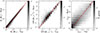 |
Fig. A.1. Comparison of the M★, SFR, and fAGN measurements (left, middle, and right panel, respectively) for the sources in the mock catalogue with the true values. The red lines indicate the 1-to-1 relations. |
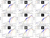 |
Fig. A.2. Examples of the CIGALE best-fit SEDs for galaxies with various levels of AGN contribution (increasing from left to right, upper to lower). The title of each panel gives the galaxy COSMOS2020 ID, redshift, reduced χ2, and the AGN fraction. Blue squares represent observed fluxes, while green triangles indicate upper limits. In each panel, we show the JWST/NIRCam F150W image of the galaxy. The cutouts have a physical size of 40 × 40 kpc and are displayed using a logarithmic stretch. |
The corresponding dispersions, computed as the MAD of the data, are 0.04, 0.06, and 0.09. Given these results, we conclude that CIGALE successfully recovers the true M★, SFR, and fAGN values of the mock sources. In Fig. ??, we display examples of the best-fit SEDs obtained with our CIGALE configuration. To illustrate the effect of different AGN fractions, we show examples with increasing fAGN, at various z.
To assess the quality of our SED fitting procedure, we compare the stellar masses obtained with the M★ computed by the COSMOS2020 team using a different SED fitting software (LePhare; Weaver et al. 2022). Figure A.3 shows an excellent agreement between the two M★ estimates, with most galaxies on the one-to-one relation. We calculate the median bias,
 (A.1)
(A.1)
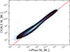 |
Fig. A.3. Comparison of the stellar mass measured by CIGALE in this work (y−axis) and the M★ provided in the COSMOS2020 catalogue, computed with LePhare (x−axis, Weaver et al. 2022). |
and the median absolute deviation (MAD),
 (A.2)
(A.2)
where ΔM★ = log10M★, LePhare − log10M★, CIGALE. We found a median bias of −0.09 and a MAD of 0.15.
Appendix B: CNN architecture
We present the CNN architecture and specific hyper-parameters adopted in this work in Table. B.1, including filter numbers and sizes, total number of trainable parameters, dropout rates, strides, and activation functions. All hyper-parameters values were chosen based on a grid search.
CNN architecture.
Appendix C: Example mergers and non-mergers
In Fig. C.1, we show some examples of galaxies labelled as mergers and non-mergers by our classifier. Galaxies are randomly selected in the two categories. In most cases, galaxies classified as mergers appear in pairs with different degrees of morphological disturbance. Non-mergers appear as isolated and regular galaxies, with spiral arms visible in some cases.
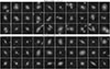 |
Fig. C.1. Random examples of galaxies classified as mergers (top 3 rows) and as non-mergers (bottom 3 rows) by our combined classifier. On top of each cutout (from the JWST/F150W images), we report the galaxy redshift and its unique ID. Cutouts have a physical size of 50 kpc × 50 kpc, displayed using a logarithmic stretch. |
Appendix D: MS – additional plots
We further explored the SFR vs stellar mass relation for AGN and non-AGN host galaxies. In Fig. D.1, we plot this relation for each AGN type, colour-coded by AGN accretion disc luminosity (Ldisc). The most luminous AGN are more likely to be hosted by star-forming galaxies than by low SFR ones, independently of AGN type. A slight correlation also appears with M★: the most luminous AGN reside in the most massive galaxies. In Fig. D.2, we show the same relation, but for MIR and X-ray AGN that are exclusively in that specific AGN class, i.e. we do not include AGN identified with multiple methods. Once again, X-ray AGN reside mostly in massive galaxies on or below the MS, while MIR AGN are in relatively less massive galaxies on or above the MS.
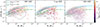 |
Fig. D.1. Contour plot illustrating the SFR vs M★ population distribution divided by AGN type, colour-coded by the AGN disc luminosity (Ldisc). In each panel, the contours (from 10% to 90%, with intervals of 10%) represent the non-AGN distribution. The dashed blue and the dash-dotted green lines indicate the MS at z = 2 and z = 0.5 from Popesso et al. (2023), respectively. |
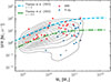 |
Fig. D.2. SFR vs M★ distribution, but in this case, both MIR and X-ray AGN types do not include the other AGN types. |
Overall, these trends reflect the general trend of AGN and non-AGN when all redshifts are combined and when overlapping between AGN types is allowed (Fig. 10). Therefore, we can conclude that: X-ray AGN are preferably hosted by giant, quenched or on the way to be quenched galaxies; MIR AGN are usually in intermediate/high M★ star-forming galaxies; SED AGN and non-AGN mostly follow the MS, but some are also found in the starburst and quenched regions.
Appendix E: Binary experiments results
In this appendix section, we report the numerical results of the merger–AGN relation adopting a binary AGN/non-AGN classification. Table E.1 shows the AGN frequency measured in mergers and non-mergers for all AGN types, divided into two redshift bins (results presented in Fig. 11). Table E.2 provides the merger fractions for all AGN types and relative non-AGN controls in the two redshift bins, as presented in Fig. 12.
Frequency of MIR-, X-ray-, and SED-selected AGN in mergers (M) and non-mergers (NM) in different redshift bins.
Merger fraction (fmerg) in galaxies hosting MIR-, X-ray-, and SED-selected AGN, and the fmerg relative to non-AGN controls.
Appendix F: fmerg–fAGN parametrisation
In this section, we detail the fitting procedure adopted to parametrise the fmerg–fAGN relation presented in LM24. In the case of MIR and X-ray AGN, we use a power law to fit the data, in the form:
 (F.1)
(F.1)
while a combination of two power laws is used for the SED AGN,
 (F.2)
(F.2)
where x = fAGN and y = fmerg. To enhance accuracy in the fits, we incorporate a sampling method. First, we uniformly sample the number of fAGN bins to divide the sample. The number of bins is drawn in the range of 6 − 20 for the X-ray and SED AGN, while the maximum number of bins allowed for the MIR AGN is set to 156. We calculate the fmerg and its uncertainty for each bin. To account for these uncertainties, which we assume follow a Gaussian distribution, we apply a bootstrapping method that varies the fractions within their errors. Next, we find the best-fit parameters for the data and repeat this process 10 000 times to ensure robustness. Finally, we calculate the best parameters as the median values of the 10 000 best fits. The best-fit parameters are reported in Table F.1.
The best-fit parameters of Eq. F.1 for X-ray and MIR AGNs, and of Eq. F.2 for SED AGNs.
All Tables
Total number of galaxies in the range 0.5 ≤ z ≤ 2 from each survey, after the MIR selection.
Frequency of MIR-, X-ray-, and SED-selected AGN in mergers (M) and non-mergers (NM) in different redshift bins.
Merger fraction (fmerg) in galaxies hosting MIR-, X-ray-, and SED-selected AGN, and the fmerg relative to non-AGN controls.
The best-fit parameters of Eq. F.1 for X-ray and MIR AGNs, and of Eq. F.2 for SED AGNs.
All Figures
|
Fig. 1. COSMOS2020 sources observed by the COSMOS-Web program. Blue rectangles indicate the tiles reduced by Zhuang et al. (2024). Red squares are the X-ray sources identified by Marchesi et al. (2016). |
| In the text | |
|
Fig. 2. Stellar mass vs redshift. The red line represents the KS-based completeness for the COSMOS2020 sample (Weaver et al. 2022). The dashed line indicates the simulations’ lower mass limit (M★ = 109 M⊙). |
| In the text | |
|
Fig. 3. Rest-frame soft (left) and hard (right) X-ray luminosities vs redshift for the selected X-ray AGN. Black arrows are upper limits. |
| In the text | |
|
Fig. 4. Left: IRAC colour–colour space. Red crosses are the selected MIR AGN. Contours show the population satisfying the 24 μm flux and S/N requirements. The blue box indicates the Chang et al. (2017) selection. Right: Rest-frame 6 μm luminosity of the AGN component vs redshift for the selected MIR AGN. |
| In the text | |
|
Fig. 5. Venn diagram of the three AGN types. |
| In the text | |
|
Fig. 6. AGN disc accretion luminosity as a function of redshift, for MIR (red crosses), X-ray (blue circles), and SED AGN (2D histogram). On the right margin, we display the Ldisc histogram distributions for the three AGN selections. |
| In the text | |
|
Fig. 7. Normalised AGN fraction distribution for the three AGN classes (SED: orange bars; X-ray: blue bars with vertical stripes; MIR: red bars with diagonal stripes) and the entire galaxy sample (dashed black line). |
| In the text | |
|
Fig. 8. Comb-CNN classification for the visually inspected test set (mergers: red circles; non-mergers: blue crosses). The scores predicted by the TNG-CNN and the HA-CNN are reported on the x- and y-axes, respectively. The shaded red or blue area defines the region of galaxies classified as mergers or non-mergers by the Comb-CNN. Sources in the white areas are labelled as unclassified. |
| In the text | |
|
Fig. 9. Comb-CNN confusion matrix for the visually inspected test set. Each cell shows the number of objects at its centre, the fraction of objects normalised by column (green percentages) in the top left corner, and the fraction of objects normalised by row (red percentages) in the lower right corner. On the main diagonal, these percentages correspond to precision and recall, respectively. |
| In the text | |
|
Fig. 10. SFR vs M★ for the three AGN types. We show the SED AGN as a 2D distribution. In each panel, the contours (from 10% to 90%, with intervals of 10%) represent the non-AGN distribution. The dashed blue and the dash-dotted green lines indicate the MS at z = 2 and z = 0.5 from Popesso et al. (2023), respectively. On top of each panel is the M★ distribution of the AGN and the corresponding non-AGN (grey). |
| In the text | |
|
Fig. 11. Top: Frequency of AGN (MIR: red; X-ray: blue; SED: orange) in mergers, indicated with filled symbols, and non-merger controls, empty symbols. Bottom: AGN frequency in mergers divided by the AGN frequency in the relative non-mergers (i.e. AGN excess). |
| In the text | |
|
Fig. 12. Merger fraction in the AGN (filled bars) and non-AGN controls (empty bars), with the same colour coding as Fig. 11. |
| In the text | |
|
Fig. 13. AGN fraction normalised distributions for mergers (orange) and non-merger controls (empty blue bars), divided by AGN type. In each panel, we display the results of the KS-test run for the two populations. |
| In the text | |
|
Fig. 14. Merger fraction as a function of AGN fraction for the MIR AGN (red crosses), X-ray AGN (blue circles), and SED AGN (orange triangles). The solid lines and coloured region show the running median and standard deviation of each relation. The dashed lines indicate the fits to the relations in LM24. The light grey area indicates the region where the relationships’ behaviours change strongly (see text). |
| In the text | |
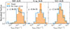 |
Fig. 15. AGN luminosity, Ldisc, normalised distributions divided by AGN type, as in Fig. 13. |
| In the text | |
|
Fig. 16. Merger fraction–AGN luminosity relation for the three AGN types. The solid line and coloured region show the running median and standard deviation of each relation. Previous literature findings are reported. |
| In the text | |
|
Fig. A.1. Comparison of the M★, SFR, and fAGN measurements (left, middle, and right panel, respectively) for the sources in the mock catalogue with the true values. The red lines indicate the 1-to-1 relations. |
| In the text | |
|
Fig. A.2. Examples of the CIGALE best-fit SEDs for galaxies with various levels of AGN contribution (increasing from left to right, upper to lower). The title of each panel gives the galaxy COSMOS2020 ID, redshift, reduced χ2, and the AGN fraction. Blue squares represent observed fluxes, while green triangles indicate upper limits. In each panel, we show the JWST/NIRCam F150W image of the galaxy. The cutouts have a physical size of 40 × 40 kpc and are displayed using a logarithmic stretch. |
| In the text | |
|
Fig. A.3. Comparison of the stellar mass measured by CIGALE in this work (y−axis) and the M★ provided in the COSMOS2020 catalogue, computed with LePhare (x−axis, Weaver et al. 2022). |
| In the text | |
|
Fig. C.1. Random examples of galaxies classified as mergers (top 3 rows) and as non-mergers (bottom 3 rows) by our combined classifier. On top of each cutout (from the JWST/F150W images), we report the galaxy redshift and its unique ID. Cutouts have a physical size of 50 kpc × 50 kpc, displayed using a logarithmic stretch. |
| In the text | |
|
Fig. D.1. Contour plot illustrating the SFR vs M★ population distribution divided by AGN type, colour-coded by the AGN disc luminosity (Ldisc). In each panel, the contours (from 10% to 90%, with intervals of 10%) represent the non-AGN distribution. The dashed blue and the dash-dotted green lines indicate the MS at z = 2 and z = 0.5 from Popesso et al. (2023), respectively. |
| In the text | |
|
Fig. D.2. SFR vs M★ distribution, but in this case, both MIR and X-ray AGN types do not include the other AGN types. |
| In the text | |
Current usage metrics show cumulative count of Article Views (full-text article views including HTML views, PDF and ePub downloads, according to the available data) and Abstracts Views on Vision4Press platform.
Data correspond to usage on the plateform after 2015. The current usage metrics is available 48-96 hours after online publication and is updated daily on week days.
Initial download of the metrics may take a while.