| Issue |
A&A
Volume 692, December 2024
|
|
|---|---|---|
| Article Number | A68 | |
| Number of page(s) | 18 | |
| Section | Planets, planetary systems, and small bodies | |
| DOI | https://doi.org/10.1051/0004-6361/202451846 | |
| Published online | 03 December 2024 | |
The distribution of the near-solar bound dust grains detected with Parker Solar Probe
Department of Physics and Technology, UiT The Arctic University of Norway,
9037,
Tromsø,
Norway
★ Corresponding author; samuel.kociscak@uit.no
Received:
9
August
2024
Accepted:
15
October
2024
Context. Parker Solar Probe (PSP) counts dust impacts in the near-solar region, but modeling effort is needed to understand the dust population’s properties.
Aims. We aim to constrain the dust cloud’s properties based on the flux observed by PSP.
Methods. We developed a forward model for the bound dust detection rates using the formalism of 6D phase space distribution of the dust. We applied the model to the location table of different PSP solar encounter groups. We explain some of the near-perihelion features observed in the data as well as the broader characteristic of the dust flux between 0.15 AU and 0.5 AU. We compare the measurements of PSP to the measurements of Solar Orbiter near 1 AU to expose the differences between the two spacecraft.
Results. We found that the dust flux observed by PSP between 0.15 AU and 0.5 AU in post-perihelia can be explained by dust on bound orbits and is consistent with a broad range of orbital parameters, including dust on circular orbits. However, the dust number density as a function of the heliocentric distance and the scaling of detection efficiency with relative speed are important to explain the observed flux variation. The data suggest that the slope of differential mass distribution, δ, is between 0.14 and 0.49. The near-perihelion observations, however, show the flux maxima, which are inconsistent with the circular dust model, and additional effects may play a role. We found an indication that the sunward side of PSP is less sensitive to the dust impacts than PSP’s other surfaces.
Conclusions. We show that the dust flux on PSP can be explained by noncircular bound dust and the detection capabilities of PSP. The scaling of flux with impact speed is especially important, and shallower than previously assumed.
Key words: Sun: corona / interplanetary medium / zodiacal dust
© The Authors 2024
 Open Access article, published by EDP Sciences, under the terms of the Creative Commons Attribution License (https://creativecommons.org/licenses/by/4.0), which permits unrestricted use, distribution, and reproduction in any medium, provided the original work is properly cited.
This article is published in open access under the Subscribe to Open model. Subscribe to A&A to support open access publication.
1 Introduction
The Parker Solar Probe (PSP) (Fox et al. 2016) and Solar Orbiter (SolO) (Müller et al. 2020) space missions are currently exploring the inner Solar System, conducting in situ measurements on an unprecedented scale and traversing regions never before reached by space probes. Through remote and in situ detections, they among others also enable unprecedented observations of the innermost region of the interplanetary dust cloud. Most of the interplanetary dust cloud originates from the asteroids and the comets of the Solar System and it is observed in the zodiacal light and its inner extension into the solar corona, called F-corona (see Koschny et al. 2019 for a recent review). While there were only a few in situ measurements of dust within 1 AU, this changed with SolO and PSP because of their experiments investigating plasma waves with antenna measurements: FIELDS (Bale et al. 2016) on PSP and Radio and Plasma Waves (RPW) (Maksimovic et al. 2020) on SolO are also sensitive to dust impacts. Earlier analyses of impact measurements of PSP (Szalay et al. 2020, 2021; Malaspina et al. 2020) and SolO (Zaslavsky et al. 2012; Kočiščák et al. 2023) showed that the observation included mainly dust on hyperbolic trajectories, which was carried away from the Sun due to the effect of the radiation pressure force, and dust in bound orbits determined by gravity. The hyperbolic grains, which are pushed outward as a result of the radiation pressure force, are often denoted as β meteoroids, since for those particles the ratio, β, of the radiation pressure force, Frp, and the gravity force, Fɡ, is roughly 0.5 or larger. Their motion is the typical central force problem, while the effective gravity force the grains are subjected to is reduced by a factor of (1 − β). Electromagnetic forces seem to have little influence in comparison, or affect only a small fraction of the dust (Mann & Czechowski 2021). It is assumed that the observed dust is created by dust-dust collisions near the Sun. This would imply that the relative amount of β meteoroids compared to dust in bound orbits decreases with increasing proximity to the Sun. We therefore investigate whether the observed dust fluxes in the close vicinity of the Sun could be due to dust in bound orbits. We also compare the dust fluxes that are observed with SolO and PSP.
The work is structured as follows. In Sect. 2, we present PSP and SolO and the previous results of other authors. We present the principle and the limitations of dust detection with electrical antennas in Sect. 3 along with the data from the two spacecraft, which we use in later analysis. In Sect. 4, we compare the dust measurements of the two spacecraft near 1 AU. In Sect. 5, we introduce the parametric forward model, which we use to explain the features observed in the dust flux measured by PSP in Sect. 6. We discuss the implications of the results in Sect. 7 and in Sect. 8 we summarize.
2 Parker Solar Probe and Solar Orbiter
2.1 Dust detection with Parker Solar Probe
PSP orbits the Sun on highly eccentric orbits between 0.05 AU and 1 AU. The orbital parameters change significantly during gravity assists, but remain nearly identical between the assists, forming several distinct orbital groups of nearly identical orbits. PSP has made 20 orbits around the Sun so far. PSP was found to be sensitive to impacts of dust grains on the spacecraft body (Szalay et al. 2020; Malaspina et al. 2020; Page et al. 2020) through the measurements of its FIELDS antenna suite (Bale et al. 2016). In addition to the electrical antennas, dust phenomena were observed with the Wide-Field Imager for PSP (WISPR) (Stenborg et al. 2021; Malaspina et al. 2022) and dust possibly damaged the Integrated Science Investigation of the Sun (IS⊙IS) instrument (Szalay et al. 2020).
It was found that the dust detection can be successfully modeled as a combination of bound dust and β meteoroids (Szalay et al. 2021). During the initial orbits, most impacts were attributed to β meteoroids. However, during the later orbits, in post-perihelia, where the relative speed between β meteoroids and the PSP is low, the dust counts are sometimes likely to be dominated by bound dust. The β value depends greatly on the grain’s size and β meteoroids have a typical size of l00 nm ≲ d ≲ 1 µm, since this is where β has its maximum (Kimura et al. 2003). The Lorentz force is negligible for β meteoroids and bound dust, due to the low Q/m < 1 × 10⁻⁷ e/mp (Czechowski & Mann 2010).
The size of the grains detected with antennas is estimated only indirectly. Based on the impact charge yields measured in laboratory hypervelocity experiments, and in combination with estimates of dust impact speed for individual dust populations based on first principles modeling, Szalay et al. (2021) estimated the lower size radius limit for detections as a function of time. They found that during orbits 8–16 of PSP, bound dust grains as small as r ≳ 300 nm near perihelia and r ≳ 2 µm near aphe-lia were detected, while β meteoroids as small as r ≳ 100 nm were detected during most of the orbit, except for post-perihelia, where the threshold was close to r ≳ 1 µm. We note that while r = 100 nm is close to the lower size limit of β meteoroids, r = 1 µm is close to the upper size limit.
Szalay et al. (2021) observed a clear double peak structure with a minimum in perihelion during orbits 4, 5, and 6 of PSP. The minimum was anticipated and at least partially explained by Szalay et al. (2020) as being due to an alignment between the nearly circular speed of bound dust and the purely azimuthal speed of PSP in the perihelion. Szalay et al. (2021) also explained the post-perihelion maximum as being potentially due to the encounter between PSP and the hypothesized Geminids β stream produced by the collisions between the bound dust cloud and the Geminids meteoroid stream.
2.2 Dust detection with Solar Orbiter
PSP’s observations of the inner zodiacal cloud are unique, and the closest available comparable observations are those of SolO (Mann et al. 2019). Similarly to PSP, SolO is equipped with electrical antennas of its RPW instrument (Maksimovic et al. 2020), which registers dust s impact on the body of the spacecraft through the dust’s electrical signatures (Soucek et al. 2021). Compared to PSP, Solo experiences much lower radial speed, and with its perihelia of about 0.3 AU, it does not go nearly as close to the Sun. Unlike PSP, the dust flux SolO measures is always dominated by β meteoroids (Zaslavsky et al. 2021; Kočiščák et al. 2023). Those were concluded to have a radius of r ≳ 100 nm (Zaslavsky et al. 2021) and β ≳ 0.5 (Kočiščák et al. 2023).
2.3 Components of the observed dust flux
One of the difficulties in explaining the observed flux is that several populations contribute to the detections (Mann et al. 2019; Szalay et al. 2020, 2021; Kočiščák et al. 2023), and therefore one must assume several components of the impact rate, which greatly decreases the fidelity of parameter estimation. As was debated by Szalay et al. (2020), bound dust and βmeteoroids are the main contributors to the dust flux on PSP. Interstellar dust grains (Mann 2010) were not yet reported by either of the spacecraft, but their presence in data is likely, even if they are a minor contributor to the overall detection counts.
A model for the β-meteoroid flux observed by both spacecraft must currently be built on many assumptions, as there are many unknowns to the population of β meteoroids. Any differences between the fluxes might be attributed to the properties of the population, or to the differences between the two spacecraft, which are numerous. The β meteoroid population was studied extensively by these spacecraft (Szalay et al. 2021; Zaslavsky et al. 2021; Kočiščák et al. 2023) and by other ones (Zaslavsky et al. 2012; Malaspina et al. 2014). Although we focus on the bound dust component, constraining this will implicitly provide information on β meteoroids, since they together make up the detected flux.
Bound dust grains are in bound orbits, and therefore have both positive and negative heliocentric speeds. In the special case of a circular orbit, the dust grain has zero heliocentric component of speed. β meteoroids are on outbound trajectories, with each of them having a positive heliocentric speed. The proportion of β meteoroids is the highest when the spacecraft has negative heliocentric speed. Conversely, the proportion of impacts of bound dust to all impacts is the highest when PSP’s radial speed is positive. The relative speed between PSP and bound dust is approximated well by PSP’s radial speed (Szalay et al. 2020), which was between 32 km s−1 and 72 km s−1 during orbital groups 1–5 between 0.15 AU and 0.5 AU. The relative speed between PSP and β meteoroids depends on their outward speed and the creation region, and was tens of km/s during the outbound legs of the studied orbits.
Szalay et al. (2020) assumed perfectly circular bound dust trajectories with β = 0 and β meteoroids originating at R0 = 5Rsun and having β = 0.5. Under these assumptions, they found the relative speed between PSP and bound dust to be higher at 0.15 AU < R < 0.5 AU for the sixth orbit and subsequent ones, compared to β meteoroids. A two-component fit to the data performed by Szalay et al. (2021) is consistent with the flux of bound dust being higher than the flux of β for 0.15 AU < R < 0.5 AU during the sixth orbit. In fact, the fit suggests that bound dust flux is more than a decade higher than in β-meteoroid flux for the sixth perihelion’s outbound leg at R = 0.2 AU. Although the exact numbers and distances are model-specific, the general trend is clear: the bound dust flux is higher than β-meteoroid flux for a good portion of the post-perihelion passage, especially for orbit 6 and later orbits.
3 Measurement technique
3.1 Antenna dust detection
When a dust grain collides with a spacecraft at a speed that exceeds a few km/s, the impact is followed by a release of a plume of a quasi-neutral charge (Friichtenicht 1962). The amount of this charge depends on many factors; most importantly, the grain s material and mass, and the impact speed. Depending on the spacecraft and the surrounding environment, a portion of the charge is collected by the spacecraft and the rest escapes from its vicinity. This process, which usually happens in µs, can be detected with fast measurements of electrical antennas, if such measurements are present. In this way, electrical antennas performing fast measurements act as dust detectors, while the whole surface of the spacecraft’s body is potentially sensitive to the impacts.
The configuration of the antennas, their location with respect to the impact site, and the material of the spacecraft surface are among the factors that influence the detection efficiency the most (Shen et al. 2023; Collette et al. 2014). Both the FIELDS instrument of PSP and the RPW instrument SolO are equipped with multiple thick cylindrical antennas close to their respective sun-facing heat shields (Bale et al. 2016; Maksimovic et al. 2020). Some of these antennas operate in the monopole configuration for both spacecraft, in which the voltage is measured between the antenna and the spacecraft body. This is the preferable configuration for dust detection, since it makes the body a more sensitive target (Meyer-Vernet et al. 2014), in comparison to dipole antennas. In dipole configuration, voltage is measured between two antennas, and such measurement is not directly sensitive to the potential of the body.
Since detections are recorded on the body of the spacecraft, the effective cross section of the body is important to establish. One of the differences between PSP and SolO is the shape. The body of SolO, excluding the solar panels, has a rough cuboid shape (ESA 2023). The body of PSP, excluding the solar panels, has a more cylindrical shape (Garcia 2018). The difference between a cuboid and a cylinder is of no consequence to dust modeling within the plane of ecliptic, but is a factor if there is an inclination between the spacecraft’s trajectory and that of the dust.
3.2 Parker Solar Probe’s potential
The potential of the spacecraft has an influence on the amplitude of the generated signal, which was studied in a laboratory previously (Collette et al. 2016; Shen et al. 2023), and this affects the detection efficiency. In the absence of a direct measurement, the floating potential of PSP can be approximated by the average of the DC voltages, Vi, between the antenna, i, and the spacecraft (Bale et al. 2020). If the antennas are on the local plasma potential, then the antennas measure voltage between the spacecraft body and the ambient plasma. The dependence of the spacecraft potential on the heliocentric distance is shown in Fig. 1. To reduce the amount of data to show, points were drawn uniformly randomly from the first 30 months of the mission and the potential was inferred this way, using DFB_WF_DC data product of FIELDS (Malaspina et al. 2016). There are many factors beyond the heliocentric distance that influence the final potential (Guillemant et al. 2012, 2013). Even so, one can see that the potential is mostly positive outside of 0.3 AU and close to zero at around 0.2 AU, and that it suddenly changes inward of 0.15 AU. The potential of PSP’s Thermal Protection System (TPS) heat shield is presumably different again, since its sunward side is not conductively coupled to the spacecraft, as is discussed in Sect. 3.3. Nevertheless, these data suggest that the dust detection process does not change significantly with the heliocentric distance, if the spacecraft is outside of 0.15 AU. This distance coincides with the distance of ≈0.16 AU, inside of which the heat shield was estimated to become conductively coupled to the spacecraft body (Diaz-Aguado et al. 2021). These two distances are possibly related.
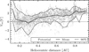 |
Fig. 1 Spacecraft potential estimated as the average of four DC antenna measurements. |
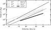 |
Fig. 2 Mass-normalized impact charge yield for several common spacecraft materials, assuming 10−14 kg dust. MLI stands for the multi-layer insulation of Solar Terrestrial Relations Observatory (STEREO). References: 1 - McBride & McDonnell (1999), 2 – Grün (1984), 3 – Collette et al. (2014), 4 – Shen (2021). All experiments were done with iron grains. |
3.3 Influence of the heat shield
Both PSP and SolO are protected from the extreme near-solar conditions by heat shields. The heat shields have different surface materials than the rest of the spacecraft. The sunward side of PSP’s TPS heat shield is, in addition, on a different potential to the rest of the body. These both influence dust detection. The sunward side of PSP’s heat shield is made of alumina, which is nonconductive and not conductively connected to the spacecraft body (Reynolds et al. 2013; Diaz-Aguado et al. 2021). The shield only becomes conductively coupled to the spacecraft body through plasma currents, once the spacecraft is inside of ≈0.16 AU (Diaz-Aguado et al. 2021). The sunward side of SolO’s heat shield is made of titanium and is conductively coupled to the rest of the spacecraft body (Damasio et al. 2015). The heat shields are exposed to dust impacts and even impacts on the nonconductive heat shield of PSP generate impact plasma (Shen 2021), which is potentially identified in the antenna measurements. Unlike impacts in the spacecraft parts connected conductively with the body ground, impacts on the heat shield only produce a dipole response, which is more directionally dependent (Shen et al. 2023) and generally weaker (Mann et al. 2019). Moreover, the amount of charge generated by impacts on the PSP’s heat shield is comparably lower, with respect to other common spacecraft materials (see Fig. 2).
3.4 Data
In the present work, we have used the data of FIELDS-detected dust counts along the trajectory of PSP, made available by Malaspina et al. (2023). The data are built on the TDSmax data product of the FIELDS instrument (Bale et al. 2016), and assume that all the fast electrical phenomena strong enough in the monopole measurement detected over quiet-enough periods of time contain dust impacts. This was demonstrated to be a good approximation of the actual dust count, with a false positive rate of about 10.5% and a miss rate of about 7% (Malaspina et al. 2023). The data are structured in intervals of 8 h, and contain the impact count in the time interval corrected for undercounting. The data also contain the total effective observation time in the 8 h interval, corrected for the time during which wave activity made dust detection ineffective. The data product is described in detail by Malaspina et al. (2023). The data from orbits 1-16, and therefore from the first five orbital groups, are examined.
In addition to the PSP data, we have also used SolO dust data. SolO detects dust with the electrical antennas of RPW instrument, and we used the convolutional neural network (CNN) data product provided by Kvammen (2022). The data product builds on the dataset of time-domain-sampled triggered electrical waveform data and was shown to have a low false positive error rate of about 4 % and a miss rate of about 3% (Kvammen et al. 2022).
Near alignments of speed and heliocentric distance between PSP and SolO.
4 PSP and SolO dust flux comparison
Although SolO and PSP have very different orbits at any given time, a direct comparison of dust fluxes can be done for several points near 1 AU, where the two spacecraft had a similar heliocentric distance and speed – albeit at different times and different helio-ecliptic latitudes. Six such time intervals were found and are listed in Table 1. Three of these are in pre-perihelion, with negative heliocentric radial speed (vr < 0) and three are in post-perihelion (vr > 0). In pre-perihelion, the ram direction of the spacecraft lies between azimuthal and sunward. The proportion of impacts on the heat shield is likely higher than in post-perihelion, when the ram direction lies between azimuthal and anti-sunward.
We compare the 14-day average flux, F, during the six alignments (7 days before and 7 days after the alignment), and the comparison is shown in Fig. 3. The flux implied by SolO is a factor of two to three higher than the flux implied by PSP. Since the flux per unit area and time are compared, the ratio depends on the cross sections, which are here assumed to be 6.11 m2 and 10.34 m2 for PSP and SolO, respectively. Part of the difference might be due to the difference between instruments and detection algorithms, leading to a different size sensitivity. The detection algorithm on PSP’s FIELDS, for example, applies a signal threshold of 50 mV (Malaspina et al. 2023), which has to be surpassed in order for detection to count. This threshold, in combination with the dust speed and mass distribution, influences the total detected counts.
One can see from Fig. 3 that the relative detection rate of PSP with respect to SolO is higher in post-perihelia than in pre-perihelia. Unlike PSP, SolO’s body is covered with conductive materials on all sides. If SolO is assumed to be equally sensitive to dust impacts from all sides, this implies that the sunward side of PSP is less sensitive than the rest of the spacecraft. This is possibly related to the nonconductive nature of the PSP’s heat shield. A less sensitive heat shield would also contribute to the lower overall flux by reducing the effective cross section of PSP.
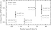 |
Fig. 3 Comparison of the 14 day cumulative flux (centered on the indicated day) observed with PSP and with SolO during their near alignments. The error bars are ±σ, bootstrapped assuming Poisson distribution. See Table 1 for the heliocentric locations, velocity components, and fluxes corresponding to the individual points. |
5 Description of the model
In this section, we present a parametric model for bound dust detection rate on a spacecraft, which we use to explain some of the observed features of the impact rate recorded on PSP. The model was built using the formalism of 6D distribution function over space r = (x, y, z) and velocity v = (vx, vy, vz): f(r, v) = f(x, y, z, vx, vy, vz), similarly to how this is done in plasma theory. A single population of bound dust is assumed. The dust number density n(r) was evaluated as
 (1)
(1)
where the unit of n is [n] = m−3. The flux, j(r), measured by the spacecraft, was evaluated as the first moment of relative speed between the spacecraft and the dust. For example, the flux through a stationary test loop oriented perpendicular to the x-axis is
 (2)
(2)
where the unit of jx is [n] = m−3 s−1. The model in this form does not include the distribution of masses, and merely assumes that all the dust grains are detected on contact with the spacecraft, regardless of the impact speed, vimpact, or grain mass, m. The focus of the model is not to explain the absolute amount of the detected dust; the model works with a multiplicative prefactor.
The spatial scaling of density, n(r), is assumed spherically symmetric:
 (3)
(3)
where r is the distance from the Sun. This allows for the presented study of the exponent, γ.
An important component of the model is the 6D distribution function, f, which describes the dust cloud and is derived in Appendix A to be in the shape
 (4)
(4)
where  is the radial speed of dust given by
 (5)
(5)
which is Eq. (A.30). The independent integration variable for the moments of f (such as Eq. (2)) was chosen to be the dust azimuthal speed, vϕ. The integration boundaries are then the lowermost and highermost speeds that the dust grains might have, given their eccentricity, e, and the effective gravity, µ(β). Therefore,
 (6)
(6)
which is Eq. (A.33).
The model captures dust’s eccentricity, e, inclination, θ, radiation pressure to gravity ratio, β, and the fraction of retrograde dust grains in the population, rp. The tilt of the dust cloud is not included, as it is not higher than a few degrees (Mann et al. 2006), and therefore inconsequential for the current effort. The model can be generalized to the out-of-ecliptic case by assuming dependence on the distance from the ecliptic plane, z. Yet, the spacecraft of interest operate very close to the ecliptic plane and the current assumption is deemed to be sufficient for the present study. The model is capable of capturing the dependence of the flux through the surface, i, denoted ji, on the impact speed by evaluating a moment different from |vimpact|. In this work, we assume the dependence
 (7)
(7)
where ϵ is the relative speed exponent, equivalent to the 1 + αδ used in several publications (Szalay et al. 2021; Zaslavsky et al. 2021; Kočiščák et al. 2023), where α is the proportionality exponent in the charge generation equation,
 (8)
(8)
and δ is the slope of the cumulative mass distribution,
 (9)
(9)
The model treats all the parameters, e; θ; β; rp; γ; ϵ, as single values (degenerate distributions). This can be, owing to the linearity, generalized to a sum of terms approximating an arbitrary distribution of these parameters, if desired. The model might in principle deal with an arbitrary shape of the spacecraft, but since the spacecraft of interest is PSP, a cylindrical shape with the axis pointing toward the Sun is assumed.
Practically, the model evaluates the flux on the spacecraft, given the position and the speed of the spacecraft. It is therefore straightforward to use the model to generate flux profiles starting with a position table of the spacecraft of interest, which is presently PSP.
The derivation of the equations and a detailed discussion of the model is provided in Appendix A. Namely: in Sect. A.1, the assumptions on the distribution function f are explained, and in Sect. A.2, the orbital dynamics equations are laid out, which are needed to integrate the flux. The integration is done in Sect. A.3 and normalization of the flux to a known number density at 1 AU is explained in Sect. A.4. Section A.5 examines the assumption of power-law scaling of perihelia dust density, which is an important assumption for the derivation. The model from Sects. A.1–A.5 includes the free parameters e; β; γ, and in Sect. A.6 we generalize the model to account for the remaining parameters, θ; rp; ϵ.
6 Observed flux and model results
In this section, we compare the post-perihelion data of each orbit with the results of the model for orbital parameters representing each of the encounter groups. These are described in Appendix B. We chose the post-perihelion region for two reasons. First, the bound dust impacts are more frequent than those of β meteoroids in this region. Second, if the sunward side of PSP is less sensitive to dust impacts, this matters the least in post-perihelia, since the sunward side is less exposed. We study post-perihelia outward of 0.15 AU, since inward the dust detection process might change, as the properties of PSP change close to the Sun, as well as to avoid the possible dust depletion zone. In the next step, we also study the near-perihelion minimum of flux observed in the data in order to see which features of the dust cloud included in the model might cause the dip.
6.1 Scaling of flux with distance
One of the features that the model should reproduce is the scaling of the observed flux with the heliocentric distance. In this section, we compare the model results to the data in the region between 0.15 AU and 0.5 AU, where the flux is dominated by bound dust impacts.
Inspection of the data shows that, with the exception of the first orbital group, which has its perihelion outside of 0.15 AU, the flux scales approximately as j ∝ R−2.5 over the outbound leg of each orbit. This is shown in Fig. 4. A variation is observed between individual orbits within the same orbital group, which was previously attributed to the stochastic nature of the dust cloud (Malaspina et al. 2020).
The base model was considered: e = 0; θ = 0; rp = 0; β = 0; γ = −1.3; ϵ = 1. This is in line with the assumption of particles on circular orbits, with no inclination, no radiation pressure, without retrograde grains, and with spatial number density scaling as n ∝ R−1.3 and the assumption that every grain is always detected, if an impact happened: j ∝vimpact. It is found that this assumption is not compatible (Fig. 5) with the slope observed in the data (Fig. 4), since the dependence produced by the model is appreciably shallower than ∝ R−2.5.
We studied which combination of parameters changes the slope to the desired ∝ R−2.5. It was found that parameters e;θ;β;rp all influence the slope in the desired direction (see Appendix C), yet even in the most favorable case they do not suffice to explain the slope observed in the data, as is shown in Fig. 5. It is also seen from Fig. 5 that the flux during the later orbits especially is influenced very little by these four parameters. The explanation therefore lies at least partially in the scaling of density with the two parameters not yet varied: the heliocentric distance exponent, γ, and the relative speed exponent, ϵ. These both influence the slope appreciably, as is seen in Figs. 6 and 7. We see that in the case of all the other parameters being equal to the base value, γ ≈ 3, or ϵ ≈ −3 show nearly flat plots, and therefore serve as upper estimates of the values. Many combinations of the six parameters are capable of reproducing the right slope. We therefore studied the range of combinations that reconstructs the slope acceptably well. A viable combination of parameters is shown in Fig. 8, but we note that the slope is not very sensitive to changes in e; θ; β; rp. Viable combinations of the most influential parameters, γ and ϵ, are shown in Fig. 9, where the other four parameters are included together in two cases: the base case, and the upper estimate, the dashed case from Fig. 5. Figure 9 shows −2 < γ < −1, which is the range of expected values of γ for bound dust (Ishimoto & Mann 1998).
We find our results compatible with previously reported γ ≈ 1.3 (Leinert et al. 1981; Stenborg et al. 2021), in which case 2 < ϵ < 2.5.
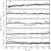 |
Fig. 4 Flux as detected by PSP in the outbound part of each orbit, compensated for by R−2 5, grouped by orbital groups. Individual encounters within a group are distinguished by markers of different shape or color. The solid lines are the power-law least squares fits to the observed flux, an exponent of which is shown in the top left corner of each panel. To demonstrate the approximate accuracy of the R−2 5 scaling, the dashed lines are the power-law fits of the data, with the exponent offset by ±0.3 from the least squares fit. |
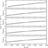 |
Fig. 5 Base model-predicted flux shown with a solid line, compensated for by R−2.5. The slope is considerably shallower than oc R−2.5; hence, the inclining trend after the compensation. The model-predicted flux in the case of e = 0.5; θ = 45°; rp = 10%; β = 0.5; γ = −1.3; ϵ = 1 is shown with the dashed line. Even these rather extreme assumptions do not suffice to explain the slope observed in the data. |
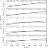 |
Fig. 6 Base model-predicted flux shown with a solid line. In addition, the influence of the heliocentric distance exponent, γ, on the slope is demonstrated. |
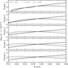 |
Fig. 7 Base model-predicted flux shown with a solid line. In addition, the influence of the velocity exponent, ϵ, on the slope is demonstrated. |
 |
Fig. 8 Base model-predicted flux shown with a solid line. In addition, the model with parameters e = 0.1; θ = 10°; rp = 0.03; β = 0.05; γ = −1.9; ϵ = 2 is shown as a representative of a viable option. |
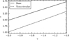 |
Fig. 9 Combinations of y and ϵ that produce a profile approximately matching the slope of −2.5 in the region of 0.15 AU < R < 0.5 AU. The base model assumes e = 0; θ = 0; rp = 0; β = 0 and the noncircular model assumes rather extreme e = 0.5; θ = 45°; rp = 0.1; β = 0.5. |
6.2 Near-Sun profile
The model is capable of reproducing features observed in the data close to perihelia. Notably, there is a distinct minimum in the measured flux in the perihelion. This minimum was attributed to the velocity alignment between PSP and bound dust (Szalay et al. 2021), which is implicitly included in the present model as well. In this section, the near-solar flux is studied as a function of the free parameters of the model.
The observational data are shown in Fig. 10 and the near-perihelion minimum is apparent. We note that the flux is not symmetric around perihelia due to the presence of β meteoroids pre-perihelia, where the relative speed between them and the spacecraft is high. We focus on the post-perihelia, as we seek to find a consistency between these and the model predictions. We also note that the PSP perihelia lie well inside the β-meteoroid creation region (Szalay et al. 2021), where the β-meteoroid grains still have an important angular momentum and their trajectories are therefore similar to the trajectories of bound dust grains, making the distinction less clear.
The base model predicted flux is shown in Fig. 11 and we note that it is symmetric around the perihelia: since only the bound dust population is assumed, and the heat shield is assumed to be as sensitive as the rest of the spacecraft, there is nothing to cause the asymmetry. The same set of vertical lines, approximately corresponding to the heliocentric locations of the maxima, are shown symmetric around the perihelia in Figs. 10 and 11. There is no post-perihelion maximum in orbital group 1; the vertical line is based solely on the pre-perihelion maximum. In the case of the base model (as before, e = 0; θ = 0; rp = 0; β = 0; γ = −1.3; ϵ = 1), the maxima in the flux are predicted to be decidedly closer to the perihelia than what is observed. It is observed in the same figure that by varying the velocity exponent, ϵ, the location of the expected maxima is moved, possibly to the extent that it is consistent with the data. None of the other parameters influences the location of the maxima of the flux appreciably and they are shown and discussed in Appendix D. They do, however, influence the relative depth of the near-perihelion flux minimum. Increasing any value except for the velocity exponent, ϵ, would result in a shallower perihelion dip (see the comparison on the influence of each individual parameter in Appendix D). We note that the dip is predicted to be shallower (approximately 50 % of the maximum) than what is observed (less than 25 % of the maximum) even in the base case.
Figure 12 shows the same combination of parameters as Fig. 8 does, which was found to be reasonable and viable to explain the observed post-perihelion slope. Even with this reasonably conservative parameter choice, the perihelion dip is a lot less pronounced, due to a less sharp alignment between the spacecraft’s and the dust’s speed. It is also observed that ϵ is less effective at changing the position of the maxima if other parameters are higher than in the base model. Therefore, we find it unlikely that the near-perihelion dip is solely due to the velocity alignment between the dust cloud and the spacecraft.
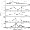 |
Fig. 10 Detection rate of dust impacts near perihelion. The data from individual solar encounters are grouped according to orbital groups. Individual encounters within a group are distinguished by markers of different shapes or colors. |
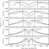 |
Fig. 11 Base model-predicted flux near the perihelia shown with a solid line. Different values of e are shown for comparison. The same vertical dashed lines as in Fig. 10 are shown for reference. |
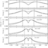 |
Fig. 12 Base model-predicted flux near the perihelia shown with a solid line. In addition, the model with parameters e = 0.1; θ = 10°; rp = 0.03; β = 0.05; y = −1.9; ϵ = 2 is shown as a representative of a viable option. |
7 Discussion
To extract physical information from the dust counts data of PSP and SolO, we performed different analyses in different helio-spheric regions. In this section, we discuss our results with respect to the heliocentric distance.
7.1 Near 1 AU
Near 1 AU, a comparison between PSP and SolO is possible and shows that PSP detects fewer dust impacts compared to SolO (see Fig. 3), especially in pre-perihelia. This is possibly an instrumental effect of smaller-sized dust being detected more effectively with SolO. As PSP’s sunward side, where the heat shield is, has a different surface material to the rest of the spacecraft, it is possibly less sensitive to dust impacts than the rest of the spacecraft (see Fig. 2). This implies that β-meteoroid impacts might be underrepresented in the data, as these are more likely to impact on the heat shield side, compared to the bound dust grains. Other instrumental effects might play a role, such as the position of antennas, and/or the presence of solar panels.
Beyond the likely instrumental cause of the difference in the flux on PSP and SolO, physical explanations are possible. Small submicron dust with r < 100 nm might be influenced by electromagnetic force. It was shown for dust of radius r ≤ 30 nm that the flux might change both with the solar cycle, which is on the order of years (Poppe & Lee 2022), and with solar rotation, which is on the order of days (Poppe & Lee 2020; Mann & Czechowski 2021) even in the case of a symmetric source. A similar, albeit weaker effect might play a role for r ≈ 100 nm dust as well. The individual points in space where we compared PSP and SolO (Fig. 3) are separated by months or weeks for a given spacecraft, and pre-perihelion and post-perihelion data points alternate in time. Therefore, a possible long-term change from 2019 to 2022 does not strongly affect the result. Due to the low number of data points, we cannot dismiss the possible influence of a well-timed short-term variation, which needs to be on the order of 25% to explain the observed difference. With the low number of points, a stochastic counting error is not negligible, but the points are based on tens and hundreds of detections, each of which are over 14 days, leading to error bars that are smaller than the observed variance.
We note that the points of similar heliocentric distance and speed between PSP and SolO lie on different heliocentric longitudes. Localized sources of β meteoroids (Szalay et al. 2021) or the interstellar dust (Mann 2010) might contribute to the difference observed between the spacecraft, although there are no indications of localized β-meteoroid sources at 1 AU. The perihelia of SolO in 2022 and 2023 are oriented close to the upstream direction of the interstellar dust, which means that more interstellar dust is likely present in the pre-perihelion data than in the post-perihelion data. The interstellar dust flux, fIS D, was reported to be coming from the heliocentric longitude of approximately λ ≈ 250 ° with the flux of fIS D < 0.036 m−2h−1 between 2016 and 2020 (Racković Babić 2022). This is an order of magnitude lower than the pre-perihelia SolO fluxes reported here (Table B.1). Although the interstellar dust might contribute to the difference, its flux is too low to explain the whole difference.
7.2 Between 0.15 AU and 0.5 AU
Between 0.15 AU and 0.5 AU, we were looking for the solutions of a parametric bound dust model, which would explain the observed slope of the detected flux. The two lines of ϵ(γ) in Fig. 9 may be regarded as upper and lower estimates of the velocity exponent, ϵ. We find that ϵ lies between 1.5 and 2.7, assuming a value for the exponent, γ, between −2 and −1. This is much lower than the previously assumed 4.15 (Szalay et al. 2021). We note that the bound dust that contributes to the results is mostly of the µm and sub-µm size. For a reasonably conservative α ≈ 3.5 (Collette et al. 2014) in ϵ = 1 + αδ, it is implied that 0.14 < δ < 0.49, which is a much lower value than δ ≈ 0.9 observed for larger dust (Grün et al. 1985; Pokorný et al. 2024). The value of α is better constrained than the value of δ. This is therefore an indication that the mass distribution may not be a single power law in the mass range of interest and at all heliocentric distances. However, this makes sense because of the narrow mass interval: the power-law distribution of masses was described over 20 decades of magnitude in mass (Grün et al. 1985), while PSP detects grains that span less than two orders of magnitude (Malaspina et al. 2023). Since the dust in question is bound, there is a necessary depletion in the small-size region, as small dust (r ≲ 100 nm) is not bound, due to high β. Interestingly, our value is compatible with δ ≈ 0.34, which was reported by Zaslavsky et al. (2021) for β meteoroids, which are also limited in mass, and the power-law distribution of masses is therefore also problematic.
We keep in mind that additional effects might influence the observed slope of ∝ R−2.5, beyond what is included in the model. However, such dependences make the interpretation of the fit values complicated and we are not aware of any findings that suggest that these other dependences are strong in the studied region. Furthermore, the solutions we found (Figs. 8 and 9) are consistent with the observed slope. The dependence of the mass distribution on distance, which influences the result, is hard to estimate, but there are indications that it changes closer to the Sun.
A recent study of the PSP/FIELDS data product (Szalay et al. 2024) found the cumulative mass distribution slope between 0.1 AU and 0.25 AU to be δ ≈ 1.1 ± 0.3, which is considerably higher than the δ < 0.49 implied by the results of this work. The work by Szalay et al. (2024) is focused on the region closer to the Sun, compared to this work (between 0.15 AU and 0.5 AU), and one of the conclusions of that work is that in the near-solar region, the value is the highest. Furthermore, the study worked with the assumption of circular grains, which in our case leads to the e, and by extension δ, being close to our upper estimate.
7.3 Near perihelia
We studied the compatibility between the bound dust model and the observed perihelion dip. A similar dip is formed due to the velocity alignment between the spacecraft and the bound dust, but the dip is too shallow and readily smeared out by nonzero eccentricity, inclination, or other parameters. It seems unlikely that the grains in the micrometer size range would be on mostly circular orbits, since β for such grains is significant (Wilck & Mann 1996) and the grains are likely formed in collisions of bigger dust grains (Ishimoto & Mann 1998). Furthermore, high-eccentricity α meteoroids were suggested (Sommer 2023) as a possible explanation of the post-perihelion flux enhancement observed by PSP during orbits 4 and 5 (Szalay et al. 2021).
If the near-perihelion dip is not due to the velocity alignment, other factors might contribute to the dip, and we list several of them. First, the dust number density is believed to diminish closer to the Sun. A dust-free zone was hypothesized to exist (Russell 1929), since the dust grains do not survive for long in the extreme conditions near the Sun. It was estimated using WISPR that a dust depletion zone enveloping the dust-free zone lies inward of 19 Rsun ≈ 0.09 AU and the dust-free zone likely lies inward of 5 Rsun ≈ 0.023 AU (Stenborg et al. 2021). Such a dust depletion zone may explain the apparent depletion of dust near perihelia.
The second possible explanation for the dip is ineffective detection. The antenna detection process is very much dependent on the spacecraft’s charge state and the surrounding environment (Shen et al. 2021; Racković Babić et al. 2022; Shen et al. 2023). An indication that the process changes rapidly inward of 0.15 AU is that the spacecraft’s potential seems to be a steep function of the heliocentric distance in this region, potentially disturbing the otherwise effective dust detection. For example, the heat shield becoming conductively coupled to the spacecraft’s body inward of ≈0.16 AU (Diaz-Aguado et al. 2021) also changes the spacecraft’s charge state (see Sect. 3.2 for the discussion of the spacecraft potential).
The third possible contribution to the dip is that if the relative speed between the dust and the spacecraft is higher than a certain threshold, all the bound dust grains are detected, and therefore the flux plateaus. This would not produce the dip on its own, but would lead to a shallower growth near the Sun compared to the case in which the proportionality of flux to ∝vϵ is assumed all the way.
In addition to these three explanations, we note that the minima near perihelion might be the result of maxima before and after perihelion, rather than a depletion. Such maxima might result from either crossing the Geminids β stream (Szalay et al. 2021), or the spacecraft getting more sensitive to dust impacts, possibly due to a higher potential (Fig. 1) and/or better sensitivity of the heat shield.
7.4 Further work
We developed a model to describe bound dust impact rates onto spacecraft, which works with sharp values for the free parameters but which is easily generalized to distributions. Other free parameters can feasibly be included, such as the tilt of the dust cloud with respect to the ecliptic plane, which might be useful for modeling the flux once the orbit of SolO becomes more inclined. Developing a similar model for dust on hyperbolic trajectories, such as β meteoroids or interstellar dust, is straightforward. The distribution of inclinations and eccentricities within β-meteoroid cloud is worthy of future investigation.
The masses are presently treated in a crude way, assuming power-law distribution of masses, which translates to the efficiency of detection. As we argue, the assumption of power-law distributed masses might not be justified. A 7D distribution function describing masses, in addition to the phase space, would offer a more nuanced model, but would push the limits of what information can possibly be retrieved from the data.
8 Conclusions
The impact rate model that we have developed in this work takes into account dust cloud parameters: the eccentricity, e, inclination, i, radiation pressure to gravity ratio, β, and retrograde dust fraction, rp. In addition, the model takes into account semiempir-ical parameters: the exponent, γ, of number density dependence on heliocentric distance and the exponent, ϵ, of the detection rate dependence on the impact speed. We compared the model results to the dust count data of the first 16 orbits of PSP.
Although the model does produce a dip in flux due to the velocity alignment between the dust and the spacecraft in the circular dust base case, the dip is not sufficient and is smeared away easily, especially with nonzero eccentricity. The dip observed close to each of the perihelia for the third and subsequent orbits of PSP in the data is not reproduced either as deeply or as widely by the model. Therefore, other effects contribute to the dip beyond the velocity alignment; namely, the dust depletion zone or instrumental effects.
The parameters of the dust cloud, e, i,β, rp, each have a minor influence on the model profile, while the semiempirical parameters, γ and ϵ, are crucial. By varying these, we can reproduce the observed dependence of flux in the post-perihelion region on the heliocentric distance between 0.15 AU and 0.5 AU, where the influence of β dust is expected to be the lowest. The parameter ϵ, which represents the combined influence of the dust mass distribution and impact charge production, is found to be lower than what was previously used for PSP dust data analysis, and likely between 1.5 and 2.7. This is consistent with the slope, δ, of differential mass distribution of µm and sub-µm dust between 0.14 and 0.49, which is shallower than what was reported for bigger bound dust further away from the Sun.
A comparison of the dust counts of PSP and SolO shows that PSP observed comparatively less dust in pre-perihelia than in post-perihelia, with a difference of about 25%. This suggests that PSP’s sun-facing side, and therefore the heat shield (TPS), offers a less dust-sensitive target compared to the other surfaces of PSP. Because of this instrumental effect, the observations are not incompatible with a stationary and symmetric dust cloud. However, due to the low number of data points, we cannot reject the possibility that the effect is physical, and attributable to short-term temporal or spatial variation in the cloud.
Acknowledgements
Author contributions: Concept: SK, AT, IM. Model development: SK, AT. Data analysis: SK, AT. Interpretation: SK, IM, AT. Manuscript preparation: SK, IM. SK and AT were supported by the Tromsø Research Foundation under the grant 19_SG_AT. This work on dust observations in the inner heliosphere received supported from the Research Council of Norway (grant number 262941 and 275503). SK appreciates the constructive discussions with Jakub Vaverka, Libor Nouzák, Jamey Szalay, Mitchell Shen, and Arnaud Zaslavsky, and the assistance of David Malaspina with interpreting the PSP dust data. The code and the data set used in this work are publicly available at https://zenodo.org/records/13284890. Authors sincerely thank the anonymous reviewer for constructive comments.
Appendix A Integrating the phase-space density
Appendix A.1 Phase-space density
Assume there is a time-invariant dust density f in the usual 6D phase space:
 (A.1)
(A.1)
which is normalized to number density as
 (A.2)
(A.2)
which is a very useful way of looking at it, since n(r) can be measured remotely for bigger (≳ 1 µm) dust grains. We note that we disregarded grain size for now, the density n represents the number density of suitable dust grains, whatever the suitability criteria are.
Since the Solar System near the ecliptic is our main goal, we will introduce simplifying assumptions on f:
We assume that the plane x ⊗ y is the ecliptic, with (0, 0) point being the Sun and assume that all the grains within the distribution move within this plane, with no poleward component of the speed vz.
We assume that the dust cloud has a rotational symmetry around the z axis, and for convenience we are going to use the density
 expressed using (r, ϕ) instead of (x, y), where
  and ϕ is the angle of rotation around z axis, measured from an arbitrary ray in the ecliptic.
We assume the dust grains don’t collide. Then we make use of Liouville’s theorem on the space (r, v).
The first assumption is translated to f using degenerate distributions δ(·) as
 (A.3)
(A.3)
The second assumption is translated using r, ϕ as
 (A.4)
(A.4)
where the first three arguments of f are all position arguments, where  has a position, angle, and a position arguments. We also use a more compact 3D distribution f, with the meaning
 (A.5)
(A.5)
since we assumed rotational symmetry in ϕ. The third assumption has the form of
 (A.6)
(A.6)
provided that the points (r1, v1), (r2, v2) (or, alternatively expressed points (r1, vr,1, vϕ,1), (r2, vr,2, vϕ,2)) share the same trajectory of the system in the phase space. We note that we use velocity, not the momentum, which is justified, since we assume the mass conservation dm/dt = 0 for each particle. We assume the dust cloud is composed of bound dust grains, each of them on a heliocentric orbit. Then Eq. A.6 holds for any two points of an orbit of a grain. If we assume all the grains follow the same gravity field with the effective gravitational parameter
 (A.7)
(A.7)
where β is the grain’s radiation pressure to gravity ratio and κMSun is the solar gravitational parameter. Then all the grains which acquire the state of (r1, v1) will also acquire the state of (r2, v2), if this a valid solution for one of them. Therefore, we may study f in a convenient point of the orbit of our choice while being assured, it remains the same throughout the orbit. We are soon going to see that the perihelion of the orbit of a dust grains is a convenient point.
Appendix A.2 Orbital mechanics
To study the density f in a point of the orbit of our choice, we must describe the orbits and be able to translate between the points within the orbit. From Eq. A.6 we know that
 (A.8)
(A.8)
provided that the spacecraft state in perihelion (rperi, 0, vperi) shares the same orbit with a general state (r, vr, vϕ). By applying the laws of orbital motion, we are going to find the relationship between the points (rperi, 0, vperi) and (r, vr, vϕ). We know the angular momentum is conserved:
 (A.9)
(A.9)
as well as the energy is
 (A.10)
Substituting vperi from the angular momentum, we get
 (A.11)
and multiplying by r2 we get
 (A.12)
The two formal solutions of this equation are
 (A.13)
where (+) and (−) correspond to the aphelion and perihelion respectively, since we didn’t assume anything other than a stationary point yet. Hence, (−) corresponds to the true rperi and substituting back for a, b, c and substituting for vperi from Eq. A.9 we get
 (A.14)
These two equations are what was needed to solve Eq. A.8. However, our goal is to study different eccentricities. Since an arbitrary distribution of eccentricities is straightforward to approximate with a linear combination of sharp-eccentricity terms, we will now focus on a sharp eccentricity e. Assuming that all the grains are not only exposed to the same effective gravity µ, but they also have the same orbital eccentricity e, it is apparent that only one speed vperi is allowed in the perihelion rperi, which conforms to the eccentricity e (★). Vis-viva equation in perihelion gives
 (A.15)
Substituting for vperi from Eq. A.9, we get
 (A.16)
This equation is the bond between an arbitrary r, vr, vϕ and the only corresponding rperi, vperi given the eccentricity e.
As a reasonable simplification (Giese et al. 1986), we assume the number density n(x,y, z) in the ecliptic depends on the heliocentric distance:
 (A.17)
where γ is a parameter, reasonably constrained by experiment. We normalized the expression by the number density at r0, which might be for example 1 AU. Assume this dependence (∝ rγ) holds for the distribution of dust grains in their perihelia (see Sect. A.5), which is surely an acceptable assumption, at least for low e, since at low e, the difference between rperi and raph is very small.
Appendix A.3 Velocity moments’ integration
The net flux of particles through the x-plane is the first speed moment
 (A.18)
The SI unit is [jx] = m−2 s−1. We are however not interested in the net flux jx but the total flux jtot,x onto the plane x. For the stationary plane x, we have
 (A.19)
Should the probe be moving in +x-direction with the speed of vp,x, the detected net flux is going to be
 (A.20)
Since we assumed all the dust being concentrated around the ecliptic plane (Eqs. A.3 and A.5),
 (A.21)
And since we align the x axis with the probe, the speed vx = vr is the radial dust speed and vy = vϕ is the azimuthal dust speed, both in the unit of translational speed (as not to confuse with the angular speed  ). The flux measured on radially oriented surfaces of the probe is
 (A.22)
and, analogically, the flux measured on the azimuthally oriented surfaces as
 (A.23)
where vp.azim is the azimuthal speed of the probe (prograde, locally in +y-direction).
To obtain the most convenient form of f in an easily integrable shape, we use two additional pieces of information: 1. the dependence on the heliocentric distance (Eq. A.17), and 2. the fact, that Eqs. A.16 and A.14 must be demanded consistent, which is the equivalent to the (★) claim. We are shortly going to integrate f over vr and vϕ, as in Eqs. A.22 and A.23. We know that not all combinations of vr, vϕ are possible given r, e. Instead of integrating in two dimensions, we will integrate in vr ⊗ vϕ space along the path vr(vϕ) given by (★). Hence, we relate Eqs. A.16 and A.14 with the goal of obtaining vr(vϕ):
 (A.24)
This quadratic equation has two solutions for vr:
 (A.25)
These solutions correspond to the radial speeds of pre-perihelion (in-going, vr < 0) and post-perihelion (out-going, vr > 0) dust, as at a given r and with a given vϕ. Since f of the dust cloud is assumed stationary, the grains do not collide and are in repetitive orbits, therefore there are exactly as many in-going as out-going.
Now to get a convenient shape of f, assuming separable power-law scaling with distance (consistently with Eq. A.17):
 (A.26)
where in the first step we expressed the condition A.25 and newly used a 2D distribution f according to  and in the second step we expressed the condition that n(r) ∝ rγ using a new
  and we lost the normalization. Since Liouville’s theorem says that the density is the same along the trajectory of the grain, it is the same in perihelion as well, and its moments are the same, and therefore integrating over z, vz, vr in an arbitrary time (LHS) and in perihelion (RHS):
 (A.27)
Since µ(1 + e) is a plain number, and except for  we only have
  and
and  and we demand the equality for arbitrary r, vϕ, the only thinkable solution for
  is of the form
 (A.28)

where the only suitable solution is b = y. Therefore,  with Eq. A.26 and Eq. A.25) give
 (A.30)
The last parenthesis of this equation may be interpreted as the integration trajectory in the vr ⊗ vϕ space. Since our integration parameter of the contraction from the vr ⊗ vϕ space to a 1D space of the path is going to be vϕ, we need the integration boundaries for vϕ. The integration boundaries are given by the lowermost and the uppermost vϕ the probe may encounter, given r,e. The lowest possible vϕ corresponds to the probe being in aphelion, whereas the highest corresponds to it being in the perihelion. We use Eq. A.25, and both in the perihelion and in the aphelion, we get vr = 0, and hence
 (A.31)
and this quadratic equation in  has two solutions:
 (A.32)
corresponding to the highest possible vϕ (in the case r is the perihelion) and the lowest possible (in the case r is the aphelion). Negative vϕ would correspond to the dust grains on retrograde orbits and are disregarded as we only want to include pro-grade dust grains for now. These are, therefore, our integration boundaries:
 (A.33)
We note that these correspond to the degenerate solutions of Eq. A.25, which makes sense, since Eq. A.25 defines a cyclic trajectory in the vr ⊗ vϕ space.
Radial flux

The expression contains two terms:  , which have the boundaries vr > vp,rad and vp,rad > vr respectively, which corresponds to flux on the sun-facing (+) and on the anti-sunward (−) respectively. We translate these boundaries from vr to vϕ in order to integrate over the parameter vϕ using the Heaviside function. Each of these two has two variants: post-perihelion (post, vr > 0) and pre-perihelion (pre, vr < 0) dust, as
  in Eq. A.25. Thus, we get four integral terms, each with a prefactor of 1/2:
 (A.35)
 (A.36)
 (A.37)
 (A.38)


We note that even and odd terms are straightforward to join as the only difference is the complementary Heaviside, but in the present shape it is easy to account for different effective areas from front and from the back of the probe in this function, since front and back terms are separated. Eqs. A.35 – A.38 are straightforward to evaluate numerically, for example with Monte Carlo integration, drawing values of vphi between the boundaries (Eq. A.33).
Azimuthal flux

The expression contains two terms:  , which have the boundaries vϕ > vp,azim and vp,azim > vϕ respectively. Since we assume prograde dust only (vϕ > 0), and pre-perihelion and post-perihelion have the same effect on the azimuthal flux, there is no further multiplication of terms, as in the case of radial flux.
![$\eqalign{ & j_{azim}^ + = \int_ {\mathop \smallint \nolimits^ _{{v_{p,azim}}}^\infty } \left( {{v_\phi } - {v_{p,azim}}} \right)v_\phi ^\gamma \delta \left( {{v_r} \pm \tilde v} \right)d{v_r}d{v_\phi } \cr & \,\,\,\,\,\,\,\,\,\, = \mathop \smallint \nolimits^ _{{v_{p,azim}}}^\infty \left( {{v_\phi } - {v_{p,azim}}} \right)v_\phi ^\gamma d{v_\phi } \cr & \,\,\,\,\,\,\,\,\,\,\,\left. { = \mathop \smallint \nolimits^ _{\max \left[ {\sqrt {{{(1 - e)\mu } \over r}} ,{v_{p,azim}}} \right]}^{\max \,\,\,\left[ {\sqrt {{{(1 + e)\mu } \over r}} ,{v_{p,azim}}} \right]}\left( {{v_\phi } - {v_{p,azim}}} \right)} \right)v_\phi ^\gamma d{v_\phi } \cr & \,\,\,\,\,\,\,\,\,\,\, = \left[ {{{v_\phi ^{\gamma + 2}} \over {\gamma + 2}} - {{v_\phi ^{\gamma + 1}{v_{p,azim}}} \over {\gamma + 1}}} \right]_{\max \left[ {\sqrt {{{(1 - e)\mu } \over r}} ,{v_{p,azim}}} \right]}^{\max \left[ {\sqrt {{{(1 + e)\mu } \over r}} ,{v_{p,azim}}} \right]}, \cr} $](/articles/aa/full_html/2024/12/aa51846-24/aa51846-24-eq67.png) (A.42)
(A.42)
![$\eqalign{ & j_{{\rm{azim }}}^ - = \int_ {\int_{ - \infty }^{{v_{p,azim}}} {\left( {{v_\phi } - {v_{p,azim}}} \right)} } v_\phi ^\gamma \delta \left( {{v_r} \pm \tilde v} \right)d{v_r}d{v_\phi } \cr & \,\,\,\,\,\,\,\,\,\, = \int_{ - \infty }^{{v_{p,{\rm{ azim }}}}} {\left( {{v_\phi } - {v_{p,azim}}} \right)} v_\phi ^\gamma d{v_\phi } \cr & \,\,\,\,\,\,\,\,\,\, = \int_{\min }^{\min } {_{\left[ {\sqrt {{{(1 - e)\mu } \over r}} ,{v_{p,azim}}} \right]}^{\left[ {\sqrt {{{(1 + e)\mu } \over r}} ,{v_{p,azim}}} \right]}} \quad \left( {{v_\phi } - {v_{p,azim)}}} \right)v_\phi ^\gamma d{v_\phi } \cr & \,\,\,\,\,\,\,\,\,\, = \left[ {{{v_\phi ^{\gamma + 2}} \over {\gamma + 2}} - {{v_\phi ^{\gamma + 1}{v_{p,azim}}} \over {\gamma + 1}}} \right]_{\min \left[ {\sqrt {{{(1 - e)\mu } \over r}} ,{v_{p,azim}}} \right]}^{\min \left[ {\sqrt {{{(1 + e)\mu } \over r}} ,{v_{p,azim}}} \right]}, \cr} $](/articles/aa/full_html/2024/12/aa51846-24/aa51846-24-eq68.png) (A.43)
(A.43)
where we very liberally ignored δ0(vr ± …), but since we integrate in vr over ℝ, it doesn’t matter where exactly this mass is accounted for. Altogether we have
 (A.44)
which is easy and straightforward to evaluate. Finally,
 (A.45)
Appendix A.4 Normalization
To normalize the flux properly to a known value of density at 1 AU in the unit of m−3, we need to evaluate the number density at r0, which might conveniently be 1 AU. If we don’t do that, then Eqs. A.35 - A.38, A.42, A.43 all vary as  for low e. Let’s evaluate n(r = r0) for the parameter e. Analogically to Eqs. A.40 and A.44:
![$\eqalign{ & \,n = \delta (z)\int_ {\int_ f } \left( {r,{v_r},{v_\phi }} \right)d{v_r}d{v_\phi }, \cr & \,\,\,\, = \delta (z)Cr_0^\gamma \int_ {\int_ {v_\phi ^\gamma } } \delta \left( {{v_r} \pm \tilde v} \right)d{v_r}d{v_\phi } \cr & \,\,\, = \delta (z)Cr_0^\gamma \int_{\sqrt {{{(1 - e)\mu \mu } \over {{r_0}}}} }^{\sqrt {{{(1 + e)\mu } \over {{r_0}}}} } {v_\phi ^\gamma } d{v_\phi } \cr & \,\,\, = \delta (z)Cr_0^\gamma \left[ {{{v_\phi ^{\gamma + 1}} \over {\gamma + 1}}} \right]_{\sqrt {{{(1 - e)\mu } \over {{r_0}}}} }^{\sqrt {{{(1 + e)\mu } \over {{r_0}}}} } \cr & \,\,\,\left. { = \delta (z)Cr_0^\gamma {1 \over {\gamma + 1}}\left[ {v_\phi ^{\gamma + 1}} \right]} \right]_{\sqrt {{{(1 - e)\mu } \over {{r_0}}}} }^{\sqrt {{{(1 + e)\mu } \over {{r_0}}}} } \cr & \,\,\, = \delta (z)Cr_0^\gamma {1 \over {\gamma + 1}}\left( {{{\left( {{{(1 + e)\mu } \over {{r_0}}}} \right)}^{{{\gamma + 1} \over 2}}} - {{\left( {{{(1 - e)\mu } \over {{r_0}}}} \right)}^{{{\gamma + 1} \over 2}}}} \right) \cr & = \delta (z)Cr_0^\gamma {1 \over {\gamma + 1}}{\left( {{\mu \over {{r_0}}}} \right)^{{{\gamma + 1} \over 2}}}\left( {{{(1 + e)}^{{{\gamma + 1} \over 2}}} - {{(1 - e)}^{{{\gamma + 1} \over 2}}}} \right). \cr} $](/articles/aa/full_html/2024/12/aa51846-24/aa51846-24-eq72.png) (A.46)
(A.46)

where [n] = m−3 at the distance of r0.
Appendix A.5 Number density assumption
To derive the fluxes following the assumption of number density scaling as n ∝ rγ, we conveniently assumed the equivalence,
 (A.48)
Here we demonstrate the validity of this assumption. Assume a dust grain is in orbit with the perihelion rperi and aphelion:
 (A.49)
where e is the eccentricity. The grain therefore spends time at the heliocentric distance, r,
 (A.50)
and the time spent, and therefore the probability 𝑔(r) the grain will be (in random time) found at r it spends at r is proportional to the inverse of the radial speed |vr|:
 (A.51)
where v and vϕ are the total and azimuthal speeds of the grain. Then we have from the vis-viva equation
 (A.52)
and vϕ is obtained using momentum conservation as
 (A.53)
where the perihelion speed vperi is also obtained from vis-viva as
 (A.54)

Obtaining r from rperi is a random process governed by the probability density function 𝑔(r|rperi). We can therefore draw a sample of rperi according to 𝑔(rperi) and transform rperi to r using the density 𝑔(r|rperi) derived here. Figure A.1 shows the γ compensated probability density function of 𝑔(rperi) before the transformation and 𝑔(r) after the transformation. A compensated density plot shows a constant, if the slope of the density is the value, for which we compensate, that is γ in our case. As is observed, the dependence n ∝ rγ is really retained after the transformation, if  is assumed.
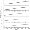 |
Fig. A.1 Sample of rperi drawn according to |

Appendix A.6 Generalization
Already included parameters The integrals for flux jtot,red and jtot, azim as derived and expressed in Sect. A.3 already allow for evaluation of the flux along a trajectory of a spacecraft, given the eccentricity of the dust’s orbits e, radiation pressure to gravity ratio β distance-scaling parameter γ and cuboid-approximated spacecraft areas, since the flux is evaluated for each of the relevant spacecraft sides independently.
Retrograde grains The simplest addition is the fraction of retrograde grains in the dust cloud. Until, now all the dust grains were considered prograde, but the fraction of retrograde dust is taken into account by weighted summing of the flux encountered along the true spacecraft trajectory, with the flux encountered by mirrored (retrograde) spacecraft trajectory.
Higher exponent of the relative speed If the detection is effective regardless of the impact speed, the flux is proportional to the relative speed between the spacecraft and the dust cloud. If the flux is assumed proportional to an exponent, ϵ, of velocity, which is higher than unity, for instance because of the detection threshold size variation with the impact speed, this is taken into account by evaluating the higher moment of (vr − vp,rad) and (vϕ − vp,azim) in the terms of Eqs. A.40 and A.44 respectively, which is straight forward. We note that the normalization needs to be adjusted in this case as well, as a scale relative velocity v0 has to be introduced, at which the number density is measured.
Inclination A single inclination angle θ different from zero can be introduced, under the assumption that all the grains share the same inclination value, albeit in different (non-parallel) orbital planes, that is with random ascending nodes. Under this assumption, a spacecraft in the ecliptic plane will only encounter dust grains of this given inclination θ. As discussed in Sect. 2.2, it is reasonable to approximate PSP by a cylinder. This makes no difference compared to a cuboid approximation, until θ ≠ 0 is examined.
We note that an arbitrary inclination of the orbital plane of each of the grains does not play a role in jtot,rad. For the azimuthal component, we need to evaluate the moment |vϕ − vp,azim| over the f, as a function of inclination θ. We assume the cylindrical symmetry,
 (A.56)
which we then need to integrate to
 (A.57)


Since by definition | · | > 0,
 (A.60)
which we evaluate easily, for example with Monte Carlo integration, drawing values of vphi between the integration boundaries (Eq. A.33).
Representative orbital parameters for PSP’s encounter groups.
We note that both nonzero eccentricity and nonzero inclination make the assumption of non-interacting grains problematic, but the collisional evolution of the dust cloud is beyond the scope of this work, and taken care of in reality by the micrometer dust cloud being constantly replenished by the product of collision of bigger grains.
Appendix B Model trajectories of PSP
Every PSP’s solar encounter is different from the previous one, even within the same orbital group. This is solely because of the motion of the Sun, which in the first approximation orbits around the common barycenter of the Sun — Jupiter system, which lies outside of the solar photosphere. PSP orbits the Sun on an orbit with perihelion distance sufficiently close to the Sun, so that this effect plays a role when the distance from the Sun is critical. This is however not as consequential as to change the results presented in this work. To get rid of the effect, we study fictitious, simplified solar encounters, which are assumed to lie in the ecliptic plane (z = 0) and which represent the actual ones well. The parameters of the encounters which we use for the present study are listen in Table B.1.
Appendix C The flux slope scaling with orbital parameters
In Sect. 6.1 we claimed that the parameters: e; θ;β; rp all act to make the slope of flux steeper, when their values differ from the base case, but in the case of the later orbits, they tend to lead to very little change. Their influence is independently shown in Figs. C.1–C.4.
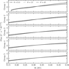 |
Fig. C.1 Base model-predicted flux (solid line). In addition, the influence of eccentricity on the slope is demonstrated. |
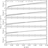 |
Fig. C.2 Base model-predicted flux (solid line). In addition, the influence of inclination on the slope is demonstrated. |
Appendix D The near-perihelia flux dependence on other parameters
In Sect. 6.2 we claimed that the parameters: e;θ;β;γ,rp do not change the location of the flux maxima appreciably. They however make the magnitude of the near-perihelia dip smaller, especially the parameter e does. Their influence is independently shown in Figs. D.1–D.5.
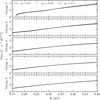 |
Fig. C.3 Base model-predicted flux (solid line). In addition, the influence of β value on the slope is demonstrated. |
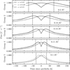 |
Fig. C.4 Base model-predicted flux (solid line). In addition, the influence of retrograde fraction on the slope is demonstrated. |
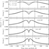 |
Fig. D.1 Base model-predicted flux (solid line). In addition, the influence of eccentricity on the slope is demonstrated. |
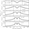 |
Fig. D.2 Base model-predicted flux (solid line). In addition, the influence of inclination is shown. |
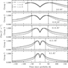 |
Fig. D.3 Base model-predicted flux (solid line). In addition, the influence of β value is shown. |
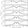 |
Fig. D.4 Base model-predicted flux (solid line). In addition, the influence of the spatial density scaling with heliocentric distance γ is shown. |
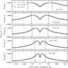 |
Fig. D.5 Base model-predicted flux (solid line). In addition, the influence of the retrograde fraction is shown. |
References
- Bale, S., Goetz, K., Harvey, P., et al. 2016, Space Sci. Rev., 204, 49 [Google Scholar]
- Bale, S., Goetz, K., Bonnell, J., et al. 2020, arXiv e-prints [arXiv:2006.00776] [Google Scholar]
- Collette, A., Grün, E., Malaspina, D., & Sternovsky, Z. 2014, J. Geophys. Res.: Space Phys., 119, 6019 [NASA ADS] [CrossRef] [Google Scholar]
- Collette, A., Malaspina, D., & Sternovsky, Z. 2016, J. Geophys. Res.: Space Phys., 121, 8182 [NASA ADS] [CrossRef] [Google Scholar]
- Czechowski, A., & Mann, I. 2010, ApJ, 714, 89 [Google Scholar]
- Damasio, C., Defilippis, P., Draper, C., & Wild, D. 2015, in 45th International Conference on Environmental Systems ICES-2015-7612-1, 6 [Google Scholar]
- Diaz-Aguado, M., Bonnell, J., Bale, S., Wang, J., & Gruntman, M. 2021, J. Geophys. Res.: Space Phys., 126, e2020JA028688 [CrossRef] [Google Scholar]
- ESA. 2023, ESA Science Satellite Fleet – Solar Orbiter 3D model, accessed: 19.3.2023 [Google Scholar]
- Fox, N., Velli, M., Bale, S., et al. 2016, Space Sci. Rev., 204, 7 [Google Scholar]
- Friichtenicht, J. 1962, Rev. Sci. Instrum., 33, 209 [NASA ADS] [CrossRef] [Google Scholar]
- Garcia, M. 2018, NASA-3D-Resources/3D Models/Parker Solar Probe, commit: 39dc094 [Google Scholar]
- Giese, R., Kneissel, B., & Rittich, U. 1986, Icarus, 68, 395 [NASA ADS] [CrossRef] [Google Scholar]
- Grün, E. 1984, in The Giotto Spacecraft Impact-induced Plasma Environment, 39 [Google Scholar]
- Grün, E., Zook, H. A., Fechtig, H., & Giese, R. 1985, Icarus, 62, 244 [NASA ADS] [CrossRef] [Google Scholar]
- Guillemant, S., Génot, V., Matéo-Vélez, J.-C., Ergun, R., & Louarn, P. 2012, Annales Geophysicae, 30, 1075 [NASA ADS] [CrossRef] [Google Scholar]
- Guillemant, S., Génot, V., Velez, J.-C. M., et al. 2013, IEEE Trans. Plasma Sci., 41, 3338 [CrossRef] [Google Scholar]
- Ishimoto, H., & Mann, I. 1998, Planet. Space Sci., 47, 225 [NASA ADS] [CrossRef] [Google Scholar]
- Kimura, H., Mann, I., & Jessberger, E. K. 2003, ApJ, 583, 314 [NASA ADS] [CrossRef] [Google Scholar]
- Kočiščák, S., Kvammen, A., Mann, I., et al. 2023, A&A, 670, A140 [NASA ADS] [CrossRef] [EDP Sciences] [Google Scholar]
- Koschny, D., Soja, R. H., Engrand, C., et al. 2019, Space Sci. Rev., 215, 1 [CrossRef] [Google Scholar]
- Kvammen, A. 2022, ML Dust Detection, https://github.com/AndreasKvammen/ML_dust_detection [Google Scholar]
- Kvammen, A., Wickstrøm, K., Kociscak, S., et al. 2022, EGUsphere [preprint], https://egusphere.copernicus.org/preprints/2022/egusphere-2022-725/ [Google Scholar]
- Leinert, C., Richter, I., Pitz, E., & Planck, B. 1981, A&A, 103, 177 [NASA ADS] [Google Scholar]
- Maksimovic, M., Bale, S., Chust, T., et al. 2020, A&A, 642, A12 [NASA ADS] [CrossRef] [EDP Sciences] [Google Scholar]
- Malaspina, D., Horányi, M., Zaslavsky, A., et al. 2014, Geophys. Res. Lett., 41, 266 [NASA ADS] [CrossRef] [Google Scholar]
- Malaspina, D. M., Ergun, R. E., Bolton, M., et al. 2016, J. Geophys. Res.: Space Phys., 121, 5088 [NASA ADS] [CrossRef] [Google Scholar]
- Malaspina, D. M., Szalay, J. R., Pokorný, P., et al. 2020, ApJ, 892, 115 [NASA ADS] [CrossRef] [Google Scholar]
- Malaspina, D. M., Stenborg, G., Mehoke, D., et al. 2022, ApJ, 925, 27 [NASA ADS] [CrossRef] [Google Scholar]
- Malaspina, D. M., Toma, A., Szalay, J. R., et al. 2023, ApJS, 266, 21 [NASA ADS] [CrossRef] [Google Scholar]
- Mann, I. 2010, ARA&A, 48, 173 [NASA ADS] [CrossRef] [Google Scholar]
- Mann, I., & Czechowski, A. 2021, A&A, 650, A29 [NASA ADS] [CrossRef] [EDP Sciences] [Google Scholar]
- Mann, I., Köhler, M., Kimura, H., Cechowski, A., & Minato, T. 2006, A&AR, 13, 159 [NASA ADS] [CrossRef] [Google Scholar]
- Mann, I., Nouzak, L., Vaverka, J., et al. 2019, Ann. Geophys., 37, 1121 [Google Scholar]
- McBride, N., & McDonnell, J. 1999, Planet. Space Sci., 47, 1005 [CrossRef] [Google Scholar]
- Meyer-Vernet, N., Moncuquet, M., Issautier, K., & Lecacheux, A. 2014, Geophys. Res. Lett., 41, 2716 [NASA ADS] [CrossRef] [Google Scholar]
- Müller, D., Cyr, O. S., Zouganelis, I., et al. 2020, A&A, 642, A1 [NASA ADS] [CrossRef] [EDP Sciences] [Google Scholar]
- Page, B., Bale, S. D., Bonnell, J., et al. 2020, ApJS, 246, 51 [NASA ADS] [CrossRef] [Google Scholar]
- Pokorný, P., Moorhead, A. V., Kuchner, M. J., Szalay, J. R., & Malaspina, D. M. 2024, Planet. Sci. J., 5, 82 [CrossRef] [Google Scholar]
- Poppe, A., & Lee, C. 2020, J. Geophys. Res.: Space Phys., 125, e2020JA028463 [NASA ADS] [CrossRef] [Google Scholar]
- Poppe, A., & Lee, C. 2022, J. Geophys. Res.: Space Phys., 127, e2022JA030317 [NASA ADS] [CrossRef] [Google Scholar]
- Racković Babić, K., Zaslavsky, A., Issautier, K., Meyer-Vernet, N., & Onic, D. 2022, A&A, 659, A15 [NASA ADS] [CrossRef] [EDP Sciences] [Google Scholar]
- Racković Babić, K. 2022, PhD thesis, Université Paris sciences et lettres; Univerzitet u Beogradu [Google Scholar]
- Reynolds, E. L., Driesman, A., Kinnison, J., & Lockwood, M. K. 2013, in AIAA Guidance, Navigation, and Control (GNC) Conference, 4879 [Google Scholar]
- Russell, H. N. 1929, ApJ, 69, 49 [Google Scholar]
- Shen, M.-H. 2021, PhD thesis, University of Colorado at Boulder [Google Scholar]
- Shen, M. M., Sternovsky, Z., Garzelli, A., & Malaspina, D. M. 2021, J. Geophys. Res.: Space Phys., 126, e2021JA029645 [Google Scholar]
- Shen, M. M., Sternovsky, Z., & Malaspina, D. M. 2023, J. Geophys. Res.: Space Phys., 128, e2022JA030981 [NASA ADS] [CrossRef] [Google Scholar]
- Sommer, M. 2023, Planet. Space Sci., 236, 105751 [NASA ADS] [CrossRef] [Google Scholar]
- Soucek, J., Píša, D., Kolmasova, I., et al. 2021, A&A, 656, A26 [CrossRef] [EDP Sciences] [Google Scholar]
- Stenborg, G., Howard, R., Hess, P., & Gallagher, B. 2021, A&A, 650, A28 [NASA ADS] [CrossRef] [EDP Sciences] [Google Scholar]
- Szalay, J., Pokorný, P., Bale, S., et al. 2020, ApJS, 246, 27 [NASA ADS] [CrossRef] [Google Scholar]
- Szalay, J., Pokorný, P., Malaspina, D., et al. 2021, Planet. Sci. J., 2, 185 [NASA ADS] [CrossRef] [Google Scholar]
- Szalay, J. R., Pokorný, P., & Malaspina, D. M. 2024, Size distribution of small grains in the inner zodiacal cloud [Google Scholar]
- Wilck, M., & Mann, I. 1996, Planet. Space Sci., 44, 493 [Google Scholar]
- Zaslavsky, A., Meyer-Vernet, N., Mann, I., et al. 2012, J. Geophys. Res.: Space Phys., 117 [CrossRef] [Google Scholar]
- Zaslavsky, A., Mann, I., Soucek, J., et al. 2021, A&A, 656, A30 [NASA ADS] [CrossRef] [EDP Sciences] [Google Scholar]
All Tables
All Figures
|
Fig. 1 Spacecraft potential estimated as the average of four DC antenna measurements. |
| In the text | |
|
Fig. 2 Mass-normalized impact charge yield for several common spacecraft materials, assuming 10−14 kg dust. MLI stands for the multi-layer insulation of Solar Terrestrial Relations Observatory (STEREO). References: 1 - McBride & McDonnell (1999), 2 – Grün (1984), 3 – Collette et al. (2014), 4 – Shen (2021). All experiments were done with iron grains. |
| In the text | |
|
Fig. 3 Comparison of the 14 day cumulative flux (centered on the indicated day) observed with PSP and with SolO during their near alignments. The error bars are ±σ, bootstrapped assuming Poisson distribution. See Table 1 for the heliocentric locations, velocity components, and fluxes corresponding to the individual points. |
| In the text | |
|
Fig. 4 Flux as detected by PSP in the outbound part of each orbit, compensated for by R−2 5, grouped by orbital groups. Individual encounters within a group are distinguished by markers of different shape or color. The solid lines are the power-law least squares fits to the observed flux, an exponent of which is shown in the top left corner of each panel. To demonstrate the approximate accuracy of the R−2 5 scaling, the dashed lines are the power-law fits of the data, with the exponent offset by ±0.3 from the least squares fit. |
| In the text | |
|
Fig. 5 Base model-predicted flux shown with a solid line, compensated for by R−2.5. The slope is considerably shallower than oc R−2.5; hence, the inclining trend after the compensation. The model-predicted flux in the case of e = 0.5; θ = 45°; rp = 10%; β = 0.5; γ = −1.3; ϵ = 1 is shown with the dashed line. Even these rather extreme assumptions do not suffice to explain the slope observed in the data. |
| In the text | |
|
Fig. 6 Base model-predicted flux shown with a solid line. In addition, the influence of the heliocentric distance exponent, γ, on the slope is demonstrated. |
| In the text | |
|
Fig. 7 Base model-predicted flux shown with a solid line. In addition, the influence of the velocity exponent, ϵ, on the slope is demonstrated. |
| In the text | |
|
Fig. 8 Base model-predicted flux shown with a solid line. In addition, the model with parameters e = 0.1; θ = 10°; rp = 0.03; β = 0.05; γ = −1.9; ϵ = 2 is shown as a representative of a viable option. |
| In the text | |
|
Fig. 9 Combinations of y and ϵ that produce a profile approximately matching the slope of −2.5 in the region of 0.15 AU < R < 0.5 AU. The base model assumes e = 0; θ = 0; rp = 0; β = 0 and the noncircular model assumes rather extreme e = 0.5; θ = 45°; rp = 0.1; β = 0.5. |
| In the text | |
|
Fig. 10 Detection rate of dust impacts near perihelion. The data from individual solar encounters are grouped according to orbital groups. Individual encounters within a group are distinguished by markers of different shapes or colors. |
| In the text | |
|
Fig. 11 Base model-predicted flux near the perihelia shown with a solid line. Different values of e are shown for comparison. The same vertical dashed lines as in Fig. 10 are shown for reference. |
| In the text | |
|
Fig. 12 Base model-predicted flux near the perihelia shown with a solid line. In addition, the model with parameters e = 0.1; θ = 10°; rp = 0.03; β = 0.05; y = −1.9; ϵ = 2 is shown as a representative of a viable option. |
| In the text | |
|
Fig. A.1 Sample of rperi drawn according to |
| In the text | |
|
Fig. C.1 Base model-predicted flux (solid line). In addition, the influence of eccentricity on the slope is demonstrated. |
| In the text | |
|
Fig. C.2 Base model-predicted flux (solid line). In addition, the influence of inclination on the slope is demonstrated. |
| In the text | |
|
Fig. C.3 Base model-predicted flux (solid line). In addition, the influence of β value on the slope is demonstrated. |
| In the text | |
|
Fig. C.4 Base model-predicted flux (solid line). In addition, the influence of retrograde fraction on the slope is demonstrated. |
| In the text | |
|
Fig. D.1 Base model-predicted flux (solid line). In addition, the influence of eccentricity on the slope is demonstrated. |
| In the text | |
|
Fig. D.2 Base model-predicted flux (solid line). In addition, the influence of inclination is shown. |
| In the text | |
|
Fig. D.3 Base model-predicted flux (solid line). In addition, the influence of β value is shown. |
| In the text | |
|
Fig. D.4 Base model-predicted flux (solid line). In addition, the influence of the spatial density scaling with heliocentric distance γ is shown. |
| In the text | |
|
Fig. D.5 Base model-predicted flux (solid line). In addition, the influence of the retrograde fraction is shown. |
| In the text | |
Current usage metrics show cumulative count of Article Views (full-text article views including HTML views, PDF and ePub downloads, according to the available data) and Abstracts Views on Vision4Press platform.
Data correspond to usage on the plateform after 2015. The current usage metrics is available 48-96 hours after online publication and is updated daily on week days.
Initial download of the metrics may take a while.