| Issue |
A&A
Volume 693, January 2025
|
|
|---|---|---|
| Article Number | A322 | |
| Number of page(s) | 11 | |
| Section | Stellar structure and evolution | |
| DOI | https://doi.org/10.1051/0004-6361/202451415 | |
| Published online | 29 January 2025 | |
LAMOST J171013+532646: A detached short-period noneclipsing hot subdwarf + white dwarf binary
1
Key Laboratory of Optical Astronomy, National Astronomical Observatories, Chinese Academy of Sciences, Beijing 100101, China
2
Yunnan Observatories, Chinese Academy of Sciences, Kunming 650011, China
3
School of Astronomy and Space Science, University of Chinese Academy of Sciences, Beijing 100049, China
4
International Centre of Supernovae, Yunnan Key Laboratory, Kunming 650216, People’s Republic of China
5
Department of Astronomy, Xiamen University, Xiamen Fujian 361005, China,
⋆ Corresponding authors; This email address is being protected from spambots. You need JavaScript enabled to view it.
; This email address is being protected from spambots. You need JavaScript enabled to view it.
Received:
7
July
2024
Accepted:
28
November
2024
Abstract
We present an analysis of LAMOST J171013.211+532646.04 (hereafter J1710), a binary system comprising a hot subdwarf B star (sdB) and a white dwarf (WD) companion. Multi-epoch spectroscopy revealed an orbital period of 109.20279 minutes, consistent with TESS and ZTF photometric data. This means that this is the sixth detached system known to harbor a WD companion with a period shorter than two hours. J1710 is remarkably close to Earth. It is situated at a distance of only 350.68−4.21+4.20 pc, with a Gaia G-band magnitude of 12.59. This renders it conducive for continuous observations. The spectral temperature is around 25 164 K, in agreement with fitting results (25301−743+839 K) based on a spectral energy distribution. The TESS light curve displays ellipsoidal variation and Doppler beaming without eclipsing features. Through fitting the TESS light curve using the Wilson-Devinney code, we determined the masses for the sdB (M1= 0.44−0.07+0.06 M⊙) and the compact object (M2= 0.54−0.07+0.10 M⊙); the compact object likely is a WD. Furthermore, MESA models suggest that the sdB, with a helium core mass of 0.431 M⊙ and a hydrogen envelope mass of 1.3 × 10⁻³ M⊙, is in the early helium main-sequence phase. The MESA binary evolution shows that the J1710 system is expected to evolve into a double WD system. This means that it is an important source of low-frequency gravitational waves.
Key words: binaries: general / subdwarfs / white dwarfs
© The Authors 2025
 Open Access article, published by EDP Sciences, under the terms of the Creative Commons Attribution License (https://creativecommons.org/licenses/by/4.0), which permits unrestricted use, distribution, and reproduction in any medium, provided the original work is properly cited.
This article is published in open access under the Subscribe to Open model. This email address is being protected from spambots. You need JavaScript enabled to view it. to support open access publication.
1. Introduction
Hot subdwarf B stars (sdBs) reside on the extreme horizontal branch in the Hertzsprung-Russell diagram. They are characterized by an extremely thin hydrogen-rich and helium-poor envelope layer and undergo helium-core burning. The typical mass of sdBs is 0.46 M⊙ (Heber 1986, 2016). Most sdBs are located in compact binaries with orbital periods Porb < 10 days (Maxted et al. 2001; Napiwotzki et al. 2004). For sdBs in binary systems, the interaction between the two companion stars is pivotal for the hot subdwarf B star (sdB) formation. Primary formation channels encompass stable Roche-lobe overflow (RLOF), common-envelope (CE) ejection, and double helium white dwarf (WD) merging. The prevailing current expectation is that short-period sdB binaries are formed by the loss of a substantial amount of angular momentum during the CE phase, which leads to the loss of most of the envelope mass (Han et al. 2002, 2003).
Kupfer et al. (2015) analyzed 142 solved sdB binaries from various samples and found that approximately half of them have WD companions. The majority of known sdB + WD binary systems has relatively long orbital periods, and little or no mass transfer occurs before the sdB evolves into a WD. Currently, only five detached systems with a WD companion are known to have Porb < 2 h (Vennes et al. 2012; Kupfer et al. 2017a,b; Pelisoli et al. 2021; Kupfer et al. 2022). However, for instance, object OW J074106.0-294811.0 has an orbital period of only 44 minutes, and the analysis suggests that its sdB might instead be a helium WD with a mass of 0.32 M⊙ (Kupfer et al. 2017a). Similar to the CD-30 ° 1122 system with a 70-minute orbital period, these compact sdB + WD binaries could be Type Ia supernova progenitors (Vennes et al. 2012; Geier et al. 2013). The most compact known sdB binary in which the sdB fills its Roche lobe is ZTF J213056.71+442046.5, with an orbital period of only 39 minutes (Kupfer et al. 2020). Furthermore, the determination of the system parameters and evolutionary stages of these systems, involving sdBs and WDs, might reveal previously unknown processes during the CE phase.
The sdB binaries may evolve into double white dwarf (DWD) systems, making them potential gravitational wave (GW) sources for space-based interferometers such as the Laser Interferometer Space Antenna (LISA), the TianQin project, and the Astrodynamical Middle-frequency Interferometric GW Observatory (AMIGO), which are designed to detect millihertz and submillihertz signals and signals at even lower frequencies. They are also expected to significantly enhance our ability to detect and study DWD systems, which will provide valuable insights into the binary evolution process before a merger (Ni 2018; Seto 2020; Amaro-Seoane et al. 2023). No GW events from DWD mergers have been detected so far. However, the LISA mission and the Taiji program (a planned space-based GW detector with a similar sensitivity and capable of operating in tandem with LISA) are expected to detect approximately 10 000 DWD systems, most of which are anticipated to lie within the frequency range of 3–6 mHz (Edwards et al. 2001; Hu & Wu 2017; Ruan et al. 2020; Cai et al. 2024; Colpi et al. 2024). The detection of GWs from individual systems during their inspiral and merger phases will deepen our understanding of the merger processes and provide new opportunities to study the detailed structure of the Milky Way (Jennrich & Binétruy 2011).
Using the Large Sky Area Multi-Object Fiber Spectroscopic Telescope (LAMOST) data, Lei et al. (2018) first identified J1710, a system containing an sdB star, and provided its basic atmospheric parameters. In this paper, we present a comprehensive analysis of J1710 using optical spectroscopy, the Gaia Data Release 3 (Gaia DR3) parallax (Gaia Collaboration 2021), and light curves from the Transiting Exoplanet Survey Satellite (TESS) (Ricker et al. 2014) and the Zwicky Transient Facility (ZTF) (Bellm et al. 2019). We conclude that it consists of an sdB star with a WD companion, with an orbital period shorter than two hours.
This paper is organized as follows. In Sect. 2 we compile and provide existing data and new observations. Section 3 describes the methods and results of our data analysis. In Sect. 4 we discuss the stellar parameters and binary evolution of J1710. Finally, our conclusions are summarized in Sect. 5. For clarity, we designate the visible sdB component, whose orbital radial velocity varies, as the primary (star 1), and the unseen WD as the secondary (star 2).
2. Observations and data reduction
2.1. Spectroscopic observations
With the release of LAMOST (Wang et al. 1996; Su & Cui 2004) DR10 data1, the total number of spectra released as of 2023 has exceeded 20 million. J1710 was observed by LAMOST on two nights in 2013 and 2016, and six subexposure spectra (R ≈ 1800) were acquired that cover the wavelength from 3700 to 9100 Å. All spectra were processed by LAMOST pipeline, and the detailed results are presented in Table 1 (Bai et al. 2017, 2021). One spectrum from 2013 was excluded because the signal-to-noise ratio (S/N) near dawn was too low (S/N = 14). The radial velocity (RV) variations in the remaining LAMOST spectra exceed 400 km/s.
Spectroscopic observations and estimated parameters of J1710.
Given the significant RV variation observed in the LAMOST spectra, J1710 was observed on three nights in 2021 using the Double Spectrograph (DBSP) instrument mounted on the 200-inch Hale Telescope (P200) at Palomar Observatory2. Eight individual spectra were acquired that covered a wavelength range of 3900–5500 Å in the blue band and 5800–7400 Å in the red band. The resolutions were approximately 2100 in the blue band and approximately 3200 in the red band. All raw data from the P200 telescope were processed using the IRAF package (Tody 1986, 1993), and the RVs were determined using the template cross-correlation method described in Bai et al. (2021).
On February 23, 2022, the Canada-France-Hawaii Telescope (CFHT)3 also conducted observations of J1710 and obtained two high-resolution spectra using ESPaDOnS (Donati et al. 2003). ESPaDOnS is an optical spectropolarimeter with a wavelength coverage between 3600 and 10 000 Å. The mean spectral resolution of the spectra is approximately 85 000, with an exposure time of 1100 s and an average S/N of about 33. The relevant information is summarized in Table 1.
2.2. Light curves
J1710, as TIC 367779738 in TESS input catalog, has been observed multiple times by TESS (Ricker et al. 2014) from 2019 to 2023 with cadences of 20, 120, 200, and 600 seconds. Given the period of approximately 109 minutes obtained from the RV analysis, data with a 120-second cadence for sectors 50–53 were downloaded from the Mikulski Archive for Space Telescopes (MAST)4. We used the SAP-FLUX light curves at 120-second cadence because their uncertainty is lower.
We retrieved the J1710 light curves from ZTF5 (Bellm et al. 2019) in the g, r, and i bands, which span four years from September 2018 to August 2022. To improve the data quality, data points with a catflags value of zero and those within one standard deviation of the mean value of the chi flag for each band were retained.
The TESS and ZTF light curves were normalized separately and were combined to yield two normalized light curves. A Lomb-Scargle periodogram analysis (Lomb 1976; Scargle 1982) was conducted using the ASTROPY library (Astropy Collaboration 2018) in Python, and we identified an orbital period of P = 109.203(3) minutes. No pulsation features were detected in the power spectrum of the TESS light curve.
3. Methods and results
3.1. Spectral parameters
We employed model spectra from previous studies that classified J1710 as an sdB (Lanz & Hubeny 2007; Nemeth et al. 2014; Hubeny & Lanz 2017) and used the UlySS package (Koleva et al. 2009; Wu et al. 2014) to fit the optical spectra of J1710 and derive stellar parameters. An example spectrum fit is shown in panel a of Fig. 1.
 |
Fig. 1. Spectrum fit of J1710. Panel a displays the LAMOST combined spectrum in the blue band (green) and its best-fitting model (red). The absorption lines of H and He are labeled. Panel b presents the fit residuals. Panel c shows fits of vrot sin i to the helium lines observed in the reduced CFHT spectra. The normalized fluxes of the single lines are shifted for clarity. |
In panel a of Fig. 1, the LAMOST spectrum (green line) exhibits prominent hydrogen Balmer and HeI lines, suggesting that the visible star likely is an sdB. Upon careful examination of the CFHT high-resolution spectra, the absence of emission line features indicates that the Roche lobe of the visible star is not filled. Several weaker lines of CII, NII, OII, MgII, AlIII, SiIII, SII, TiIII, VIII, and FeIII were identified. A more detailed analysis of the metallicity is beyond the scope of this work.
The best-fitting parameters for each observed spectrum were determined by minimizing the χ2 value, and they are listed in Table 1. The mean and standard deviation of these parameters were calculated and adopted as the final values: Teff = 25164 ± 663 K, log g = 5.68 ± 0.08 dex, and log(n(He)/n(H)) = −2.26 ± 0.09 dex. The CFHT spectra had an exposure time of 1100 s, accounting for 17% of the period, and their S/N is low and significantly affects the broadening of the absorption lines. Therefore, a Gaussian smoothing was applied to the CFHT spectra to reduce the resolution to 25 000. Additionally, based on the RV curve fit in Sect. 3.2, corrections for long exposures were applied to the CFHT spectra. The RV at each second of the exposure was calculated and added to the model spectra. These velocity-shifted spectra were then summed and normalized before they were compared to the observed spectra. From the four HeI lines (4026, 4471, 4921, and 5875 Å), the projected rotational velocity vrot sin i was determined to be 89 ± 12 km/s, as shown in panel c of Fig. 1 and summarized in Table 2.
Summaries of the parameters for J1710.
3.2. Orbital parameters
We corrected for phase smearing of the RV data from the spectra following the method outlined in Yuan et al. (2023). The corrected RVs were then analyzed using TheJoker (Price-Whelan et al. 2017), yielding an orbital period P = 109.20279 ± 0.00003 minutes, an eccentricity e = 0.013 ± 0.011, an RV semi-amplitude K1 = −223.3 ± 3.8 km/s, and a systemic velocity V0 = −40.5 ± 7.3 km/s. The corrected RV values are provided in Table 1.
Considering J1710 as a compact binary system with a short period and a nearly circular orbit (e ≈ 0), we assumed the orbit to be circular (e = 0). Using the aforementioned orbital parameters as priors and fixing the period at P = 109.20279 minutes, we fit the phase-folded RVs with a sinusoid and performed a Markov hain Monte Carlo (MCMC) sampling. The derived orbital parameters are  km/s, V0 = −36.5 ± 2.0 km/s, and T0 = 2459744.03573 ± 0.00012 days, as presented in Fig. 2.
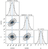 |
Fig. 2. Results of the sinusoidal RV fit using the MCMC technique. The eccentricity e is fixed to 0. For convenience, T0* is defined as (T0 − 2459744.03573)×10 000. The derived reference ephemeris is T0 = 2459744.03573 ± 0.00012 days, with an RV semi-amplitude of |

Using the parameters from the best light-curve fit (see Section 3.5), we performed an MCMC analysis on the TESS light curve by varying the period and T0. The light curve generated by the Wilson-Devinney code was expressed in phase and flux, while the observed TESS light curve was expressed in time (dates) and flux. To compare the two, the observed light curve was folded into the phase domain for each combination of period and T0. We then used the MCMC sampling to evaluate the match between the theoretical and observed light curves. The resulting ephemeris is
 (1)
(1)
where E corresponds to the epoch, and ϕ = 0 marks the point when the visible star is farthest from the observer. Given the continuous and densely sampled TESS data from four sectors, the derived T0 is highly accurate, and this ephemeris was adopted as the final one.
When P = 109.20279 minutes and K = 222.2 km/s, with e = 0, the binary mass function is
 (2)
(2)
where q = M2/M1 denotes the mass ratio, and i signifies the orbital inclination.
3.3. Spectral energy distribution fit
The correction of the Gaia DR3 (Gaia Collaboration 2023) parallax of J1710 to ϖ = 2.85 ± 0.03 mas according to Lindegren et al. (2021) yields a distance of 350.87 ± 3.70 pc. Based on this distance, the Bayestar2019 map (Green et al. 2019) provides values of E(B − V) = 0.018, 0.018, and 0.027 for the 16th, 50th, and 84th percentiles of the reddening at this coordinate, respectively. Additionally, based on the 2D dust maps by Schlegel et al. (1998) and Planck Collaboration Int. XLVIII (2016), we identified E(B − V) values of 0.013 and 0.02. Combining this information, we adopted E(B − V) = 0.018 ± 0.01 and used this as a prior to fit the spectral energy distribution (SED).
The SED of the visible star was fit using the models from the TüBingen NLTE Model-Atmosphere Package (TMAP) (Werner et al. 2012). In the left panel of Fig. 3, we combined the photometric data spanning from the ultraviolet to the infrared, and the SED was accurately fit with a model of a single sdB (red line).
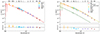 |
Fig. 3. SED fit of J1710. The left panel displays the broad SED and observed photometry for the single sdB component (red), and the right panel includes an additional WD component (green). However, aligning the Galaxy Evolution Explorer (GALEX) photometry values in the right panel results in a deviation of the total flux (yellow) from the observed photometry in other bands. The photometric data sources include GALEX (Lasker et al. 2008), Gaia (synthetic photometry derived from Gaia BP/RP mean spectra in the Sloan Digital Sky Survey (SDSS) u-band, aquamarine; Gaia Collaboration 2022), the AAVSO Photometric All-Sky Survey (APASS) (Henden et al. 2015), the Two Micron All-Sky Survey (2MASS) (Cutri et al. 2003), and the Wide-field Infrared Survey Explorer (WISE) (W1 and W2, brown; Cutri et al. 2021). The Pan-STARRS (PS1) observations of J1710 in the g, r, i, z, and y bands (12.67, 13.04, 13.31, 13.35, and 13.62 mag) obtained through the VizieR Photometry Viewer exceeded the limiting magnitudes for bright stars in these bands, as indicated in Table 11 of Chambers et al. (2016), except for the y band. Therefore, APASS photometric data were used instead of PS1 data. |
An MCMC approach was used to minimize the residuals between the observational SED and the TMAP model, enabling the derivation of errors on the parameters. We adopted prior assumptions for the effective temperature, surface gravity, and distance. The best-fitting parameters include the effective temperature  , which is consistent with the value obtained from the spectral fitting (Teff = 25164 K), reddening
  , radius R1 = 0.164 ± 0.004 R⊙, distance
  , and luminosity log(L/L⊙) = 1.00 ± 0.03. The results of this analysis are presented in Fig. 4, and these parameters are listed in Table 2.
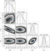 |
Fig. 4. Corner plot of the SED fit results for J1710 with a single component using the TMAP model. |
Using the Koester model (Koester 2010) to account for the flux contribution from the companion WD, we show the result in the right panel of Fig. 3. The sdB model flux remains consistent with that in the left panel. At a WD temperature of 46 848 K, the total model flux (yellow line) shows residuals close to zero in the ultraviolet band compared to the SED. However, significant deviations are observed in other bands, and the companion star contributes approximately 4% of the flux in the optical bands. Thus, the MCMC analysis likely only captured the parameters of the visible star, indicating that the effective temperature of the companion WD is probably lower than 46 848 K. Consequently, the luminosity of the companion WD can be neglected.
3.4. Extinction and kinematics
Based on the extinction law of Cardelli et al. (1989) and the effective wavelengths of various bands, when considering  , the extinctions calculated in the g, r, i, Gaia G, and TESS bands are listed in Table 2. The mean apparent magnitude and absolute magnitude in the Gaia G band are 12.59 and 4.81 ± 0.04, respectively.
The proper motion for J1710 provided by Gaia DR3 is pmra = 0.75 ± 0.05 mas/yr and pmdec = −13.34 ± 0.05 mas/yr. Additionally, the system velocity is −36.5 ± 2.0 km/s, resulting in a 3D motion in LSR of −28.6 ± 0.3 km/s, −20.5 ± 1.2 km/s, −14.9 ± 0.9 km/s, indicating a thin-disk object (Pthin ≈ 98.3%) (Johnson & Soderblom 1987; Ramírez et al. 2013). We employed the bootstrapping method to estimate the uncertainties.
3.5. Light-curve fit
Using the established ephemeris, the TESS data were phase-folded and rebinned into 400 data points, and the ZTF data were phase-folded for each band. The resulting normalized light curves are shown in Fig. 5, where the ellipsoidal variation in the primary star dominates. Additionally, Doppler beaming is observed, which leads to an asymmetric light curve due to the large RV amplitude. This in turn results in a higher flux when the visible star approaches Earth compared to when it moves away (Hermes et al. 2012).
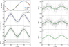 |
Fig. 5. Folded RV curve, normalized light curves, and model light curves in the ZTF g, r, and i bands and in the TESS band. The photometric data points are represented as black points in all folded light curves. The gray shading indicates the errors. The model light curves generated from the Wilson-Devinney code are depicted in green for their respective bands. Panel a1 illustrates the calculated RV curve using the best-fit values K1 = 222.2 km/s and Vsys = −36.5 km/s. Detailed spectroscopic information is provided in Table 1. Panel b1 displays the fitting results when the inclination is highest and the companion star temperature is highest. The model light curve is shown in blue. No significant features of the companion star are discernible. Panel c1 presents the TESS light curve and the well-fit model light curve. The companion star temperature is fixed at 20 000K and the other parameters are set to their mean values, as described in the main text. The residuals are depicted in panel d1. Panels a2, b2, and c2 show the ZTF light curves and the corresponding model light curves. |
To determine the binary properties, the Wilson-Devinney code (Wilson & Devinney 1971; Wilson 1979, 1990, 2012) was used to fit the TESS light curves and RVs simultaneously. Assuming a circular orbit and synchronized stellar rotation periods with the orbital period, we obtained the projected rotational velocity vrot sin i = 89 ± 12 km/s, corresponding to an orbital inclination  . In this compact binary system composed of an sdB and a WD, the reflection effect is negligible because the WD is much smaller.
Some additional information was incorporated as input for the orbital solution. The orbital period was fixed to 109.20279 minutes, as derived in Section 3.2. The primary star temperature was constrained to 25 301 K, as determined in Sect. 3.3. Additionally, the primary star radius, obtained from high-precision SED fitting and Gaia parallax data, served as a reliable reference. The limb-darkening coefficients in logarithmic form (e = 0.27, f = 0.15) and the Doppler-beaming coefficients (β = 1.47) were fixed based on the tables of Claret et al. (2020), with values closest to the atmospheric parameters for the TESS filter. Given the high effective temperature of the primary star, the gravity-darkening exponent (GR) and bolometric albedo (ALB) were set to one. The companion star has no visible observational features. Its temperature was fixed at 20 000 K, and a large potential Ω2 was assigned to ensure a small radius.
Through 50 000 bootstrap-fitting samples, the uncertainty of the orbital solution was evaluated, and the final results are presented in Fig. 6. The mass ratio q, semimajor axis (SMA), orbital inclination i, and the gravitational potential of the visible star Ω1 were treated as free parameters. The orbital inclination  , distance D = 350.68 ± 4.20 pc, and extinction AT = 0.022 ± 0.014 were sampled using Gaussian distributions. For each set of sampled parameters, the code iterated to derive optimal values for the semimajor axis SMA, mass ratio q, gravitational potential Ω1, and the corresponding inclination i. The derived values are
  ,
,  , R1 = 0.164 ± 0.002 R⊙, SMA = 0.75 ± 0.01 R⊙,
  , and
, and  dex, with the optimal zeropoint flux in the TESS-band CALIB of 0.1734 erg s−1 cm−3. The sdB star fills approximately 61% of its Roche lobe. Due to the absence of eclipses in the light curve, larger uncertainties remain for parameters such as the mass. The best-fitting model is shown in panel c1 of Fig. 5.
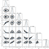 |
Fig. 6. Bootstrapping sampling results for the TESS band light curve using the Wilson-Devinney code. The diagonal elements present the probability distribution of each parameter. The percentiles of 16%, 50%, and 84% are denoted by vertical lines. Star 1 denotes the visible component, and star 2 denotes the invisible compact component. The uncertainties in inclination, distance, extinction, gravity darkening, and other parameters were all considered. See the text for more details. |
To assess the impact of the companion star temperature and orbital inclination on the light-curve fitting, the orbital inclination was fixed at its maximum value, i = 68°, while the temperature of the companion star was adjusted to its maximum value, T2 = 46 848 K, as depicted in panel b1 of Fig. 5. Under these conditions, the model light curve (blue line) remains consistent with the TESS data (black dots) and shows no distinctive features. Consequently, this scenario does not provide additional constraints on parameters such as the temperature of the companion star. Thus, as discussed in Sect. 3.3, the flux contribution from the companion star was disregarded. For all other cases, the temperature of the companion star was held constant at T2 = 20 000 K. With the inclination fixed at 55° and considering the effects of ellipsoidal variation and Doppler beaming, as shown in panel c1, the model light curve (green line) fits the TESS data well. the residuals are depicted in panel d1.
According to Eggleton (1983), the Roche radius of the companion can be approximated as
 (3)
(3)
where a is the orbital separation between the two stars. Kepler’s third law relates the orbital separation and period. For M2 ranging from 0.47 to 0.64 M⊙, the Roche radius RRL2 varies from 0.28 to 0.32 R⊙, all of which is smaller than the radii of main-sequence stars with a corresponding mass. The absence of emission lines in the spectra suggests that J1710 does not exhibit strong mass transfer, indicating that the companion must be a WD with a radius smaller than its Roche radius.
J1710 is saturated in the PS1 images in the g, r, and i bands and falls within the ZTF saturation limits of approximately 12.5 to 13.2 magnitudes6 (Chambers et al. 2016; Masci et al. 2019). Moreover, the ZTF magnitudes exhibit significant scatter, which makes the data unreliable for a light-curve fitting. Therefore, using the best-fit parameters from the light-curve model, synthetic light curves were generated in the g, r, and i bands, were normalized, and were compared with the observed ZTF light curves. Since the ZTF magnitudes are calibrated using the PS1 system (Masci et al. 2019), the ZTF magnitudes were converted in to SDSS using the PS1-to-SDSS relation (Tonry et al. 2012), as shown in panels a2, b2, and c2 of Fig. 5. The amplitudes of the J1710 light curves are influenced by various factors, including the temperature and ellipticity of the primary star, the relative sizes of the stars, and the surface brightness. The model light curves in these three bands (green lines) generally agree with the ZTF data (black dots; the gray lines represent the errors). This validates the reliability of our results.
4. Discussions
4.1. Modeling the sdB
The system position in the color-magnitude diagram is depicted in the left panel of Fig. 7. Different samples are represented by different colors: green for sdB, blue for sdO, and gold for sdOB, following the definitions provided in Lei et al. (2021), with respective sample sizes of 169, 22, and 63. The sample of objects within a radius of 100 parsec is depicted as gray points, consistent with the approach used in Pelisoli & Vos (2019), where they were shown as black points in their Figure 1. The comparison with Figure 1 of Heber (2016) further emphasizes that the visible star in J1710 is an sdB.
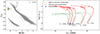 |
Fig. 7. Color-magnitude diagram and evolutionary tracks for five sdB models derived from a 2.16 M⊙ main-sequence progenitor. In the left panel, the gray data points represent sources within 100 parsecs in the Gaia DR3 dataset, and the green, blue, and gold points indicate candidate sources identified as sdB, sdO, and sdOB stars, respectively. The right panel shows MESA evolutionary tracks of sdB model stars with different hydrogen envelope masses, with or without convective overshooting. When the helium core mass is 0.431 M⊙ and the envelope mass is 0.0013 M⊙, the evolutionary track covers the observed data and corresponding 1σ error region. |
The results we obtained so far suggest that J1710 comprises a compact binary system hosting an sdB with a period shorter than two hours. The visible star is estimated to have a mass of  , and the companion star, a WD, is estimated to have a mass of
  . According to the classical formation theory of sdBs, the primary energy loss mechanism involves the ejection of the sdB hydrogen envelope through a CE phase (Han et al. 2002, 2003; Heber 2016). This process significantly reduces the orbital period.
To understand the current evolutionary status of the sdB, we used the code Modules for Experiments in Stellar Astrophysics (MESA), specifically, version r23.05.1 (Paxton et al. 2011, 2013, 2015, 2018, 2019; Jermyn et al. 2023), to model single-star evolution. The models were initialized with a metallicity Z = 0.02 and initial masses ranging from 1 to 5 M⊙, starting from the pre-main-sequence phase. For simplicity, atomic diffusion mixing, stellar wind, and rotation were excluded. At the tip of the red giant branch, the built-in tool named relax mass was used to artificially remove the hydrogen envelope with the aim to determine the helium core mass and hydrogen envelope mass at the birth of the sdB. This procedure matches the current observational parameters of the visible star ( , log(L/L⊙) = 1.00 ± 0.03).
When we modeled the evolution of sdBs and considered convective overshooting, we applied an exponential overshoot with the recommended value from Herwig (2000) (fov = 0.016) at all convective boundaries, with the mixing length parameter α set to 1.8. This resulted in breathing pulsations when the core helium abundance (Yc) was lower than 0.2. These pulsations can cause fluctuations in the core size with stellar luminosity and radius (Caloi 1989; Li & Li 2021). Despite the long recognition of breathing pulsations, uncertainties persist, and they might be numerical artifacts rather than genuine physical phenomena (Paxton et al. 2019). Therefore, for reference, we also modeled the sdBs without overshooting. The stellar evolution calculations were terminated when helium was depleted at the stellar center (Yc < 10−3).
The right panel of Fig. 7 shows that for an initial stellar mass of 2.16 M⊙, the sdB model (comprising a 0.431 M⊙ helium core and a 0.0013 M⊙ hydrogen envelope) closely matches the observed parameters of the visible star (indicated by the blue cross). This result is based on the specific MESA version and the physical parameter settings used in our analysis. For other typical sdB models, for instance, one with a mass of 0.47 M⊙, the temperature, luminosity, and log g values do not correspond to the observed data presented in Sect. 3. The sdB parameters derived from our model are Teff = 25 284 K, log(L/L⊙) = 1, log g = 5.64 dex, and R1 = 0.164 R⊙, with an age of approximately 12 Myr in the sdB phase. These parameters are highly consistent with the observed results in Sect. 3, and this confirms the robustness and reliability of the results we obtained.
4.2. Binary evolution
We employed the MESA binary evolution module to evolve the sdB and WD in J1710 together to investigate when the sdB would fill its Roche lobe, and whether J1710 would evolve into an AM CVn system, or alternatively, whether GW radiation dominates orbital shrinkage, leading to a DWD system merger. Assuming fully conservative mass transfer from the sdB to the WD during the RLOF phase, we followed the mass-transfer rates prescribed by Ritter (1988). All angular momentum losses were assumed to arise from gravitational wave radiation.
The current sdB models were obtained as described in Sect. 4.1, with evolutionary tracks stopping when they reached the observed Teff and log(L/L⊙) values. Because we lack detailed information about the WD, we adopted the results from the SED fit in Sect. 3.3. The fit suggests that the WD temperature is below 46 848 K. Assuming an sdB mass of 0.432 M⊙, we determined the WD mass to be 0.54 M⊙ based on the mass function. We constructed a WD model with a C/O core using the make_co_wd test case in MESA, and evolved a 0.54 M⊙ WD model until log(L/L⊙) = − 1.2, where the WD temperature is approximately 23 701 K, consistent with the SED fit. The initial orbital period was set to 109.20279 minutes, and the evolution was halted when the luminosity of the primary (sdB) dropped below log(L/L⊙) = − 1. The final results, shown in Fig. 8, indicate that the J1710 system will evolve into a DWD and will eventually merge.
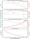 |
Fig. 8. Binary evolution of J1710 from the present day until the sdB star evolves into a WD, modeled using the MESA code. In the top two panels, the moment when the sdB phase ends is marked with a star. In each subplot, the green lines correspond to the left vertical axis, and the red lines correspond to the right vertical axis. Detailed descriptions of the panels are provided in Sect. 4.2. |
Fig. 8 illustrates the binary system evolution from the present until the sdB becomes a WD. The top panel shows the evolution of the primary star luminosity (green line) and central density (red line) over time. Approximately 89 Myr from now, when the core helium abundance of the sdB drops to Yc < 10−3 (marked with a star), the sdB phase ends and the star transitions to the WD phase. When the primary luminosity falls below log(L/L⊙) = − 1 and its central density exceeds 6 g cm−3, the sdB has fully transformed into a WD.
The second panel displays the Roche-lobe filling factor (green line) and the mass of the sdB (red line) over time. The Roche-lobe filling factor, defined as the ratio of the sdB radius to its Roche-lobe radius, remains below one throughout the evolution, indicating that no significant mass transfer occurs. Moreover, the sdB mass remains constant, which further confirms the absence of mass exchange before the system becomes a DWD. Thus, no AM CVn system is formed.
The third panel shows the orbital period (green line) and its decay (red lines) over time. The red lines compare the orbital period decay predicted by the MESA model with that expected from GW radiation alone. The lines overlap, indicating that orbital shrinkage and angular momentum loss are solely driven by GW emission. The fourth panel illustrates the decreasing temperature (green line) and luminosity (red line) of the WD as it cools over time. The results demonstrate that the sdB star will not fill its Roche lobe before it becomes a WD, and no mass transfer occurs in the system.
When the primary star has a mass of M1 = 0.432 M⊙ and the secondary has a mass of  , GW radiation is the only mechanism for orbital shrinkage, ultimately leading to the merger of the two degenerate companions. The merger timescale for such a double-degenerate system can be estimated using the following formula (Chandra et al. 2021):
 (4)
(4)
With an orbital period of 1.82 hours, the merger timescale ranges from 180 to 231 Myr, which roughly matches the evolutionary age of the system indicated in Fig. 8. This confirms that the J1710 binary system will merge within a Hubble time.
4.3. In the absence of tidal synchronization
Tidal synchronization is a debated topic for stars with convective cores and radiative envelopes like sdBs, as the exact dissipation mechanisms remain elusive. In Sect. 3.5 we assumed tidal synchronization. The tidal synchronization time can be estimated simply as (Hilditch 2001)
![Mathematical equation: $$ \begin{aligned} t_{\text{ sync}} = 10^4 \left[\frac{(1+q)}{2q}\right]^2 P^4, \end{aligned} $$](/articles/aa/full_html/2025/01/aa51415-24/aa51415-24-eq32.gif) (5)
(5)
where tsync is in years. For an orbital eccentricity e = 0, q = M2/M1 = 1.24 as derived in Sect. 3.5, and P = 109.20279 minutes, the synchronization time is about 0.27 years. Therefore, J1710 likely reaches tidal synchronization very quickly.
However, current observations suggest that tidal synchronization has not been achieved in many sdB binaries. For example, in the J162256+473051 system, the orbital period is 0.069789 days, while the rotation period is 0.115156 days, indicating that the sdB star rotation is not synchronized with its orbital motion (Schaffenroth et al. 2014). A similar nonsynchronous behavior is observed in other systems, such as KIC 11179657 (Pablo et al. 2012) and PG1142-037 (Reed et al. 2016), which also display longer rotation periods than expected for synchronization. These observations further reinforce the notion that tidal synchronization is a rare feature in many sdB binary systems.
Moreover, Preece et al. (2018) estimated the tidal synchronization timescale using tidal dissipation theories that account for dissipation via turbulent convection. Their results suggest that in most observed cases, the synchronization timescale significantly exceeds the lifetime of the sdB star. However, recent work by Ma & Fuller (2024) challenges these assumptions, particularly in regard to the treatment of tidal dissipation through gravity waves. While earlier models such as those by Geier et al. (2010), Pablo et al. (2012), and Preece et al. (2018) assumed efficient damping of gravity waves near the stellar surface, Ma & Fuller (2024) suggested that these waves may be less effectively damped than previously thought, potentially leading to much faster tidal synchronization. Their findings indicate that the synchronization timescale is primarily determined by the orbital period, with a weaker dependence on the mass of the companion star.
Although the tidal synchronization assumption in Sect. 3.5 yields an sdB mass consistent with the MESA models from Sect. 4.1, we cannot entirely rule out the possibility that J1710 is not tidally synchronized because we lack additional observational data. In the absence of tidal synchronization, the sdB star rotational period would be expected to exceed the orbital period, allowing for higher orbital inclinations than when tidal synchronization is present. With a repeated fit of the TESS light curve and RV data simultaneously using the Wilson-Devinney code, and permitting the orbital inclination i to vary between 45° and 90°, we find an inclination of i = 67 ° ±15°, with 1σ uncertainties yielding  ,
,  , R1 = 0.164 ± 0.002 R⊙, SMA = 0.75 ± 0.01 R⊙,
  , and
, and  dex. These results remain consistent with the MESA model predictions within the error margins. Thus, while the absence of tidal synchronization introduces additional uncertainties in determining the orbital parameters, it does not alter the conclusion that J1710 is a compact sdB+WD binary system with an orbital period of shorter than 2 hours.
4.4. Gravitational waves
Considering the maximum possible companion star mass M2 = 0.64 M⊙ for the J1710 binary system, with M1 = 0.432 M⊙, and P = 109.20279 minutes, the dimensionless GW amplitude (𝒜) is calculated from Shah et al. (2012) as
 (6)
(6)
where the GW frequency fgw = 2/P, and the distance d = 350.68 pc. This yields fgw ≈ 0.3 mHz and a dimensionless GW amplitude 𝒜 ≈ 2 × 10⁻²².
The characteristic strain amplitude hc of J1710 based on four years of LISA observations can be calculated using the formula (Moore et al. 2015)
 (7)
(7)
where Tobs = 4 years. This results in a characteristic strain hc ≈ 4 × 10⁻²⁰. Unfortunately, this falls notably short of the sensitivity threshold outlined in the LISA sensitivity curve (see Figure 3 in Kupfer et al. (2018) and Figure 5 in Chandra et al. (2021)). Nonetheless, the GW signal emitted by J1710 will introduce additional foreground noise, which will affect the LISA sensitivity curve (Amaro-Seoane et al. 2023). We anticipate that future space-based GW observatories will detect more short-period WD binaries and their merger events. This will enhance our understanding of DWD evolution.
5. Conclusion
We provided a comprehensive analysis of the nearby compact binary system J1710, which comprises an sdB and a WD. The system has a short orbital period of 109.20279(7) minutes, less than 2 hours, and is located at a distance of  from Earth. Through spectroscopic, SED, and light-curve fitting, the visible star was identified as an sdB with a temperature
  , a radius R1 = 0.164 ± 0.002 R⊙, and a luminosity log(L/L⊙) = 1 ± 0.03. The visible star mass was determined to be
  through light-curve fitting, while the MESA model covering the observed temperature and luminosity indicated M1 = 0.432 M⊙. The system membership in the thin-disk binary population was suggested by the dynamic analysis.
In the absence of direct evidence for the companion star, its mass varies with the orbital inclination. As indicated in Sect. 3.5, the companion star mass was estimated to be  , and it was identified as a WD. As described in Sect. 1, only six detached systems with a WD companion and Porb < 2 h have undergone comprehensive analysis, including J1710. Excluding CD-30 ° 1122, which is at a distance of
  (Deshmukh et al. 2024), J1710 is the closest at
  . Furthermore, its Gaia G-band mean magnitude stands at 12.59, indicating exceptional brightness and making it a prime candidate for additional observations. The abundance of observational data might augment our comprehension of the condition and evolution of these compact binary systems.
High-resolution ultraviolet and optical observations of J1710 with a high S/N could enhance our comprehension of its evolutionary trajectory and unveil distinctive post-CE phase characteristics. It is anticipated to undergo evolution into a DWD system and eventually merge, thus emerging as a pivotal source of low-frequency GWs for space-based observatories.
Acknowledgments
This work is supported by the National Natural Science Foundation of China (12273056, 12090041, 11933004) and the National Key R&D Program of China (2019YFA0405002, 2022YFA1603002). HL.Y and ZR.B are supported by the National Key R&D Program of China (Grant No. 2023YFA1607901). HL.Y acknowledges support from the Youth Innovation Promotion Association of the CAS (Id. 20200060) and National Natural Science Foundation of China (Grant No. 11873066). ZW.L and XF.C are supported by the National Natural Science Foundation of China (NSFC, Nos. 12288102, 12473034, 12125303, 12090040/3), the National Key R&D Program of China (Nos. 2021YFA1600403/1 and 2021YFA1600400), the Yunnan Fundamental Research Projects (Nos. 202401AT070139, 202201AU070234, 202101AU070276), the Natural Science Foundation of Yunnan Province (Nos. 202201BC070003, 202001AW070007), the International Centre of Supernovae, Yunnan Key Laboratory (No. 202302AN360001), and the “Yunnan Revitalization Talent Support Program”-Science and Technology Champion Project (No. 202305AB350003). We also acknowledge the science research grant from the China Manned Space Project with No.CMS-CSST-2021-A10. Guoshoujing Telescope (the Large Sky Area Multi-Object Fiber Spectroscopic Telescope LAMOST) is a National Major Scientific Project built by the Chinese Academy of Sciences. Funding for the project has been provided by the National Development and Reform Commission. LAMOST is operated and managed by the National Astronomical Observatories, Chinese Academy of Sciences. This work presents results from the European Space Agency (ESA) space mission Gaia. Gaia data are being processed by the Gaia Data Processing and Analysis Consortium (DPAC). Funding for the DPAC is provided by national institutions, in particular the institutions participating in the Gaia MultiLateral Agreement (MLA). The Gaia mission website is https://www.cosmos.esa.int/gaia. The Gaia archive website is https://archives.esac.esa.int/gaia. This work uses data obtained through the Telescope Access Program (TAP), which has been funded by the TAP member institutes. We would like to acknowledge and thank TAP (ID: CTAP2022-A0018) for their support. We acknowledge use of the VizieR catalog access tool, operated at CDS, Strasbourg, France, and of Astropy, a community-developed core Python package for Astronomy (Astropy Collaboration 2013, 2018).
References
- Amaro-Seoane, P., Andrews, J., Arca Sedda, M., et al. 2023, Liv. Rev. Relat., 26, 2 [NASA ADS] [CrossRef] [Google Scholar]
- Astropy Collaboration (Robitaille, T. P., et al.) 2013, A&A, 558, A33 [NASA ADS] [CrossRef] [EDP Sciences] [Google Scholar]
- Astropy Collaboration (Price-Whelan, A. M., et al.) 2018, AJ, 156, 123 [Google Scholar]
- Bai, Z., Zhang, H., Yuan, H., et al. 2017, PASP, 129, 024004 [NASA ADS] [CrossRef] [Google Scholar]
- Bai, Z.-R., Zhang, H.-T., Yuan, H.-L., et al. 2021, RAA, 21, 249 [NASA ADS] [Google Scholar]
- Bellm, E. C., Kulkarni, S. R., Graham, M. J., et al. 2019, PASP, 131, 018002 [Google Scholar]
- Cai, R.-G., Guo, Z.-K., Hu, B., et al. 2024, Fundam. Res., 4, 1072 [NASA ADS] [CrossRef] [Google Scholar]
- Caloi, V. 1989, A&A, 221, 27 [NASA ADS] [Google Scholar]
- Cardelli, J. A., Clayton, G. C., & Mathis, J. S. 1989, ApJ, 345, 245 [Google Scholar]
- Chambers, K. C., Magnier, E. A., Metcalfe, N., et al. 2016, arXiv e-prints [arXiv:1612.05560] [Google Scholar]
- Chandra, V., Hwang, H.-C., Zakamska, N. L., et al. 2021, ApJ, 921, 160 [NASA ADS] [CrossRef] [Google Scholar]
- Claret, A., Cukanovaite, E., Burdge, K., et al. 2020, A&A, 634, A93 [EDP Sciences] [Google Scholar]
- Colpi, M., Danzmann, K., Hewitson, M., et al. 2024, arXiv e-prints [arXiv:2402.07571] [Google Scholar]
- Cutri, R. M., Skrutskie, M. F., van Dyk, S., et al. 2003, VizieR Online Data Catalog, II/246 [Google Scholar]
- Cutri, R. M., Wright, E. L., Conrow, T., et al. 2021, VizieR Online Data Catalog, II/328 [Google Scholar]
- Deshmukh, K., Bauer, E. B., Kupfer, T., & Dorsch, M. 2024, MNRAS, 527, 2072 [Google Scholar]
- Donati, J. F. 2003, in Solar Polarization, eds. J. Trujillo-Bueno, & J. Sanchez Almeida, ASP Conf. Ser., 307, 41 [Google Scholar]
- Edwards, T., Sandford, M. C. W., & Hammesfahr, A. 2001, Acta Astronaut., 48, 549 [NASA ADS] [CrossRef] [Google Scholar]
- Eggleton, P. P. 1983, ApJ, 268, 368 [Google Scholar]
- Gaia Collaboration (Brown, A. G. A., et al.) 2021, A&A, 649, A1 [NASA ADS] [CrossRef] [EDP Sciences] [Google Scholar]
- Gaia Collaboration 2022, VizieR Online Data Catalog, I/360 [Google Scholar]
- Gaia Collaboration (Vallenari, A., et al.) 2023, A&A, 674, A1 [NASA ADS] [CrossRef] [EDP Sciences] [Google Scholar]
- Geier, S., Heber, U., Podsiadlowski, P., et al. 2010, A&A, 519, A25 [NASA ADS] [CrossRef] [EDP Sciences] [Google Scholar]
- Geier, S., Marsh, T. R., Wang, B., et al. 2013, A&A, 554, A54 [NASA ADS] [CrossRef] [EDP Sciences] [Google Scholar]
- Green, G. M., Schlafly, E., Zucker, C., Speagle, J. S., & Finkbeiner, D. 2019, ApJ, 887, 93 [NASA ADS] [CrossRef] [Google Scholar]
- Han, Z., Podsiadlowski, P., Maxted, P. F. L., Marsh, T. R., & Ivanova, N. 2002, MNRAS, 336, 449 [Google Scholar]
- Han, Z., Podsiadlowski, P., Maxted, P. F. L., & Marsh, T. R. 2003, MNRAS, 341, 669 [NASA ADS] [CrossRef] [Google Scholar]
- Heber, U. 1986, A&A, 155, 33 [NASA ADS] [Google Scholar]
- Heber, U. 2016, PASP, 128, 082001 [Google Scholar]
- Henden, A. A., Levine, S., Terrell, D., & Welch, D. L. 2015, Am. Astron. Soc. Meeting Abstr., 225, 336.16 [Google Scholar]
- Hermes, J. J., Kilic, M., Brown, W. R., Montgomery, M. H., & Winget, D. E. 2012, ApJ, 749, 42 [NASA ADS] [CrossRef] [Google Scholar]
- Herwig, F. 2000, A&A, 360, 952 [NASA ADS] [Google Scholar]
- Hilditch, R. W. 2001, An Introduction to Close Binary Stars (Cambridge, UK: Cambridge University Press) [Google Scholar]
- Hu, W.-R., & Wu, Y.-L. 2017, Natl. Sci. Rev., 4, 685 [CrossRef] [Google Scholar]
- Hubeny, I., & Lanz, T. 2017, arXiv e-prints [arXiv:1706.01859] [Google Scholar]
- Jennrich, O., Binétruy, P., & Colpi, M., et al. 2011, NGO (New Gravitational Wave Observatory) Assessment Study Report, Tech. rep., ESA/SRE [Google Scholar]
- Jermyn, A. S., Bauer, E. B., Schwab, J., et al. 2023, ApJS, 265, 15 [NASA ADS] [CrossRef] [Google Scholar]
- Johnson, D. R. H., & Soderblom, D. R. 1987, AJ, 93, 864 [Google Scholar]
- Koester, D. 2010, Mem. Soc. Astron. Italiana, 81, 921 [NASA ADS] [Google Scholar]
- Koleva, M., Prugniel, P., Bouchard, A., & Wu, Y. 2009, A&A, 501, 1269 [CrossRef] [EDP Sciences] [Google Scholar]
- Kupfer, T., Geier, S., Heber, U., et al. 2015, A&A, 576, A44 [NASA ADS] [CrossRef] [EDP Sciences] [Google Scholar]
- Kupfer, T., Ramsay, G., van Roestel, J., et al. 2017a, ApJ, 851, 28 [NASA ADS] [CrossRef] [Google Scholar]
- Kupfer, T., van Roestel, J., Brooks, J., et al. 2017b, ApJ, 835, 131 [NASA ADS] [CrossRef] [Google Scholar]
- Kupfer, T., Korol, V., Shah, S., et al. 2018, MNRAS, 480, 302 [NASA ADS] [CrossRef] [Google Scholar]
- Kupfer, T., Bauer, E. B., Marsh, T. R., et al. 2020, ApJ, 891, 45 [Google Scholar]
- Kupfer, T., Bauer, E. B., van Roestel, J., et al. 2022, ApJ, 925, L12 [NASA ADS] [CrossRef] [Google Scholar]
- Lanz, T., & Hubeny, I. 2007, ApJS, 169, 83 [CrossRef] [Google Scholar]
- Lasker, B. M., Lattanzi, M. G., McLean, B. J., et al. 2008, AJ, 136, 735 [Google Scholar]
- Lei, Z., Zhao, J., Németh, P., & Zhao, G. 2018, ApJ, 868, 70 [Google Scholar]
- Lei, Z., Zhao, J., Nemeth, P., & Zhao, G. 2021, VizieR Online Data Catalog, J/ApJ/881/135 [Google Scholar]
- Li, Z., & Li, Y. 2021, ApJ, 923, 166 [NASA ADS] [CrossRef] [Google Scholar]
- Lindegren, L., Bastian, U., Biermann, M., et al. 2021, A&A, 649, A4 [EDP Sciences] [Google Scholar]
- Lomb, N. R. 1976, Ap&SS, 39, 447 [Google Scholar]
- Ma, L., & Fuller, J. 2024, arXiv e-prints [arXiv:2408.16158] [Google Scholar]
- Masci, F. J., Laher, R. R., Rusholme, B., et al. 2019, PASP, 131, 018003 [Google Scholar]
- Maxted, P. F. L., Heber, U., Marsh, T. R., & North, R. C. 2001, MNRAS, 326, 1391 [CrossRef] [Google Scholar]
- Moore, C. J., Cole, R. H., & Berry, C. P. L. 2015, CQG, 32, 015014 [NASA ADS] [CrossRef] [Google Scholar]
- Napiwotzki, R., Karl, C. A., Lisker, T., et al. 2004, Ap&SS, 291, 321 [NASA ADS] [CrossRef] [Google Scholar]
- Nemeth, P., Östensen, R., Tremblay, P., & Hubeny, I. 2014, in 6th Meeting on Hot Subdwarf Stars and Related Objects, eds. V. van Grootel, E. Green, G. Fontaine, & S. Charpinet, ASP Conf. Ser., 481, 95 [Google Scholar]
- Ni, W.-T. 2018, Eur. Phys. J. Web Conf., 168, 01004 [NASA ADS] [CrossRef] [EDP Sciences] [Google Scholar]
- Pablo, H., Kawaler, S. D., Reed, M. D., et al. 2012, MNRAS, 422, 1343 [NASA ADS] [CrossRef] [Google Scholar]
- Paxton, B., Bildsten, L., Dotter, A., et al. 2011, ApJS, 192, 3 [Google Scholar]
- Paxton, B., Cantiello, M., Arras, P., et al. 2013, ApJS, 208, 4 [Google Scholar]
- Paxton, B., Marchant, P., Schwab, J., et al. 2015, ApJS, 220, 15 [Google Scholar]
- Paxton, B., Schwab, J., Bauer, E. B., et al. 2018, ApJS, 234, 34 [NASA ADS] [CrossRef] [Google Scholar]
- Paxton, B., Smolec, R., Schwab, J., et al. 2019, ApJS, 243, 10 [Google Scholar]
- Pelisoli, I., & Vos, J. 2019, MNRAS, 488, 2892 [Google Scholar]
- Pelisoli, I., Neunteufel, P., Geier, S., et al. 2021, Nat. Astron., 5, 1052 [NASA ADS] [CrossRef] [Google Scholar]
- Planck Collaboration Int. XLVIII. 2016, A&A, 596, A109 [NASA ADS] [CrossRef] [EDP Sciences] [Google Scholar]
- Preece, H. P., Tout, C. A., & Jeffery, C. S. 2018, MNRAS, 481, 715 [NASA ADS] [CrossRef] [Google Scholar]
- Price-Whelan, A. M., Hogg, D. W., Foreman-Mackey, D., & Rix, H.-W. 2017, ApJ, 837, 20 [NASA ADS] [CrossRef] [Google Scholar]
- Ramírez, I., Allende Prieto, C., & Lambert, D. L. 2013, ApJ, 764, 78 [CrossRef] [Google Scholar]
- Reed, M. D., Baran, A. S., Østensen, R. H., et al. 2016, MNRAS, 458, 1417 [Google Scholar]
- Ricker, G. R., Winn, J. N., Vanderspek, R., et al. 2014, in Space Telescopes and Instrumentation 2014: Optical, Infrared, and Millimeter Wave, eds. J. Oschmann, M. Jacobus, M. Clampin, G. G. Fazio, & H. A. MacEwen, SPIE Conf. Ser., 9143, 914320 [Google Scholar]
- Ritter, H. 1988, A&A, 202, 93 [NASA ADS] [Google Scholar]
- Ruan, W.-H., Liu, C., Guo, Z.-K., Wu, Y.-L., & Cai, R.-G. 2020, Nat. Astron., 4, 108 [NASA ADS] [CrossRef] [Google Scholar]
- Scargle, J. D. 1982, ApJ, 263, 835 [Google Scholar]
- Schaffenroth, V., Geier, S., Heber, U., et al. 2014, A&A, 564, A98 [NASA ADS] [CrossRef] [EDP Sciences] [Google Scholar]
- Schlegel, D. J., Finkbeiner, D. P., & Davis, M. 1998, ApJ, 500, 525 [Google Scholar]
- Seto, N. 2020, Phys. Rev. D, 102, 123547 [NASA ADS] [CrossRef] [Google Scholar]
- Shah, S., van der Sluys, M., & Nelemans, G. 2012, A&A, 544, A153 [NASA ADS] [CrossRef] [EDP Sciences] [Google Scholar]
- Su, D.-Q., & Cui, X.-Q. 2004, Chinese J. Astron. Astrophys., 4, 1 [Google Scholar]
- Tody, D. 1986, in Instrumentation in astronomy VI, ed. D. L. Crawford, SPIE Conf. Ser., 627, 733 [Google Scholar]
- Tody, D. 1993, in Astronomical Data Analysis Software and Systems II, eds. R. J. Hanisch, R. J. V. Brissenden, & J. Barnes, ASP Conf. Ser., 52, 173 [Google Scholar]
- Tonry, J. L., Stubbs, C. W., Lykke, K. R., et al. 2012, ApJ, 750, 99 [Google Scholar]
- Vennes, S., Kawka, A., O’Toole, S. J., Németh, P., & Burton, D. 2012, ApJ, 759, L25 [Google Scholar]
- Wang, S.-G., Su, D.-Q., Chu, Y.-Q., Cui, X., & Wang, Y.-N. 1996, Appl. Opt., 35, 5155 [NASA ADS] [CrossRef] [Google Scholar]
- Werner, K., Dreizler, S., & Rauch, T. 2012, TMAP: Tübingen NLTE Model-Atmosphere Package, Astrophysics Source Code Library [record ascl:1212.015] [Google Scholar]
- Wilson, R. E. 1979, ApJ, 234, 1054 [Google Scholar]
- Wilson, R. E. 1990, ApJ, 356, 613 [Google Scholar]
- Wilson, R. E. 2012, AJ, 144, 73 [Google Scholar]
- Wilson, R. E., & Devinney, E. J. 1971, ApJ, 166, 605 [Google Scholar]
- Wu, Y., Du, B., Luo, A., Zhao, Y., & Yuan, H. 2014, in Statistical Challenges in 21st Century Cosmology, eds. A. Heavens, J. L. Starck, & A. Krone-Martins, 306, 340 [NASA ADS] [Google Scholar]
- Yuan, H., Li, Z., Bai, Z., et al. 2023, AJ, 165, 119 [NASA ADS] [CrossRef] [Google Scholar]
All Tables
All Figures
|
Fig. 1. Spectrum fit of J1710. Panel a displays the LAMOST combined spectrum in the blue band (green) and its best-fitting model (red). The absorption lines of H and He are labeled. Panel b presents the fit residuals. Panel c shows fits of vrot sin i to the helium lines observed in the reduced CFHT spectra. The normalized fluxes of the single lines are shifted for clarity. |
| In the text | |
|
Fig. 2. Results of the sinusoidal RV fit using the MCMC technique. The eccentricity e is fixed to 0. For convenience, T0* is defined as (T0 − 2459744.03573)×10 000. The derived reference ephemeris is T0 = 2459744.03573 ± 0.00012 days, with an RV semi-amplitude of |
| In the text | |
|
Fig. 3. SED fit of J1710. The left panel displays the broad SED and observed photometry for the single sdB component (red), and the right panel includes an additional WD component (green). However, aligning the Galaxy Evolution Explorer (GALEX) photometry values in the right panel results in a deviation of the total flux (yellow) from the observed photometry in other bands. The photometric data sources include GALEX (Lasker et al. 2008), Gaia (synthetic photometry derived from Gaia BP/RP mean spectra in the Sloan Digital Sky Survey (SDSS) u-band, aquamarine; Gaia Collaboration 2022), the AAVSO Photometric All-Sky Survey (APASS) (Henden et al. 2015), the Two Micron All-Sky Survey (2MASS) (Cutri et al. 2003), and the Wide-field Infrared Survey Explorer (WISE) (W1 and W2, brown; Cutri et al. 2021). The Pan-STARRS (PS1) observations of J1710 in the g, r, i, z, and y bands (12.67, 13.04, 13.31, 13.35, and 13.62 mag) obtained through the VizieR Photometry Viewer exceeded the limiting magnitudes for bright stars in these bands, as indicated in Table 11 of Chambers et al. (2016), except for the y band. Therefore, APASS photometric data were used instead of PS1 data. |
| In the text | |
|
Fig. 4. Corner plot of the SED fit results for J1710 with a single component using the TMAP model. |
| In the text | |
|
Fig. 5. Folded RV curve, normalized light curves, and model light curves in the ZTF g, r, and i bands and in the TESS band. The photometric data points are represented as black points in all folded light curves. The gray shading indicates the errors. The model light curves generated from the Wilson-Devinney code are depicted in green for their respective bands. Panel a1 illustrates the calculated RV curve using the best-fit values K1 = 222.2 km/s and Vsys = −36.5 km/s. Detailed spectroscopic information is provided in Table 1. Panel b1 displays the fitting results when the inclination is highest and the companion star temperature is highest. The model light curve is shown in blue. No significant features of the companion star are discernible. Panel c1 presents the TESS light curve and the well-fit model light curve. The companion star temperature is fixed at 20 000K and the other parameters are set to their mean values, as described in the main text. The residuals are depicted in panel d1. Panels a2, b2, and c2 show the ZTF light curves and the corresponding model light curves. |
| In the text | |
|
Fig. 6. Bootstrapping sampling results for the TESS band light curve using the Wilson-Devinney code. The diagonal elements present the probability distribution of each parameter. The percentiles of 16%, 50%, and 84% are denoted by vertical lines. Star 1 denotes the visible component, and star 2 denotes the invisible compact component. The uncertainties in inclination, distance, extinction, gravity darkening, and other parameters were all considered. See the text for more details. |
| In the text | |
|
Fig. 7. Color-magnitude diagram and evolutionary tracks for five sdB models derived from a 2.16 M⊙ main-sequence progenitor. In the left panel, the gray data points represent sources within 100 parsecs in the Gaia DR3 dataset, and the green, blue, and gold points indicate candidate sources identified as sdB, sdO, and sdOB stars, respectively. The right panel shows MESA evolutionary tracks of sdB model stars with different hydrogen envelope masses, with or without convective overshooting. When the helium core mass is 0.431 M⊙ and the envelope mass is 0.0013 M⊙, the evolutionary track covers the observed data and corresponding 1σ error region. |
| In the text | |
|
Fig. 8. Binary evolution of J1710 from the present day until the sdB star evolves into a WD, modeled using the MESA code. In the top two panels, the moment when the sdB phase ends is marked with a star. In each subplot, the green lines correspond to the left vertical axis, and the red lines correspond to the right vertical axis. Detailed descriptions of the panels are provided in Sect. 4.2. |
| In the text | |
Current usage metrics show cumulative count of Article Views (full-text article views including HTML views, PDF and ePub downloads, according to the available data) and Abstracts Views on Vision4Press platform.
Data correspond to usage on the plateform after 2015. The current usage metrics is available 48-96 hours after online publication and is updated daily on week days.
Initial download of the metrics may take a while.