| Issue |
A&A
Volume 692, December 2024
|
|
|---|---|---|
| Article Number | A162 | |
| Number of page(s) | 13 | |
| Section | Planets, planetary systems, and small bodies | |
| DOI | https://doi.org/10.1051/0004-6361/202451252 | |
| Published online | 10 December 2024 | |
Revisiting the conundrum of the sub-Jovian and Neptune desert
A new approach that incorporates stellar properties
1
Dipartimento di Fisica “Ettore Pancini”, Università di Napoli Federico II,
Napoli,
Italy
2
INFN, Sezione di Napoli, Complesso Universitario di Monte S. Angelo,
Via Cintia Edificio 6,
80126
Napoli,
Italy
3
INAF – Osservatorio Astronomico di Capodimonte,
via Moiariello 16,
80131
Napoli,
Italy
4
INAF – Osservatorio Astrofisico di Catania,
Via S. Sofia 78,
95123
Catania,
Italy
5
Science and Technology Department, Parthenope University of Naples,
Naples
80143
Italy
6
European Southern Observatory,
Karl-Schwarzschild-Strasse 2
85748
Garching bei Munchen, Munchen,
Germany
7
Fakultat fúr Physik, Ludwig-Maximilians-Universität München,
Scheinerstraße 1,
81679
Munchen,
Germany
8
INAF, Osservatorio Astrofisico di Arcetri,
Largo E. Fermi 5,
50125,
Firenze,
Italy
9
UNESCO Chair “Environment, Resources and Sustainable Development”, Department of Science and Technology, Parthenope University of Naples,
Naples,
Italy
★ Corresponding author; christian.magliano@unina.it
Received:
25
June
2024
Accepted:
18
November
2024
Context. The search for exoplanets has led to the identification of intriguing patterns in their distributions, one of which is the so-called sub-Jovian and Neptune desert. The occurrence rate of Neptunian exoplanets with an orbital period P ≲ 4 days sharply decreases in this region in period-radius and period-mass space.
Aims. We present a novel approach to delineating the sub-Jovian and Neptune desert by considering the incident stellar flux F on the planetary surface as a key parameter instead of the traditional orbital period of the planets. Through this change of perspective, we demonstrate that the incident flux still exhibits a paucity of highly irradiated Neptunes, but also captures the proximity to the host star and the intensity of stellar radiation.
Methods. Leveraging a dataset of confirmed exoplanets, we performed a systematic analysis to map the boundaries of the sub-Jovian and Neptune desert in the (F, Rp) and (F, Mp) diagrams, with Rp and Mp corresponding to the planetary radius and mass, respectively. By using statistical techniques and fitting procedures, we derived analytical expressions for these boundaries that offer valuable insights into the underlying physical mechanisms governing the dearth of Neptunian planets in close proximity to their host stars.
Results. We find that the upper and lower bounds of the desert are well described by a power-law model in the (F, Rp) and (F, Mp) planes. We also obtain the planetary mass-radius relations for each boundary by combining the retrieved analytic expressions in the two planes. This work contributes to advancing our knowledge of exoplanet demographics and to refining theoretical models of planetary formation and evolution within the context of the sub-Jovian and Neptune desert.
Key words: methods: statistical / astronomical databases: miscellaneous / planets and satellites: general
© The Authors 2024
 Open Access article, published by EDP Sciences, under the terms of the Creative Commons Attribution License (https://creativecommons.org/licenses/by/4.0), which permits unrestricted use, distribution, and reproduction in any medium, provided the original work is properly cited.
This article is published in open access under the Subscribe to Open model. Subscribe to A&A to support open access publication.
1 Introduction
One of the most intriguing features in the various findings in the realm of exoplanetary science is the scarcity of exoplanets that spans from sub-Jupiters to super-Earths at small orbital distances (period of ≲4 days). This is known as the hot sub-Jovian/ Neptune desert (e.g. Mazeh et al. 2016; Szabó & Kiss 2011). We adopt this nomenclature here. Mazeh et al. (2005) first pointed out that a negative linear relation exists between the planetary mass and the orbital period. As more planets were discovered in the following years, several other authors examined this tendency (e.g. Szabó & Kiss 2011; Beaugé & Nesvorný 2013) and broadened this correlation to the planetary radius (e.g. Beaugé & Nesvorný 2013; Mazeh et al. 2016). In particular, Szabó & Kiss (2011) found a sparsely populated region in the P− Mp diagram with P ≤ 2.5 days, spanning 0.02–0.8 MJ, which they termed the sub-Jovian desert. Similar findings were also obtained by Beaugé & Nesvorný (2013), who extended the analysis to the P – Rp diagram: this diagram shows that planets with 3 R⊕ ≤ Rp ≤ 11R⊕ that orbit their host star in ≲4 days are very rare. These works pointed out that this region is constrained by two boundaries: an upper boundary delimited by hot Jupiters, and a lower boundary consisting of super-Earths and sub-Neptunes. Mazeh et al. (2016) obtained an analytic description of the two boundaries delimiting the desert in the log P − log Mp and log P − log Rp planes. Although the debate about the origin of the desert is still ongoing, the distribution of close-in exoplan-ets is the result of a non-trivial combination of atmospheric and dynamical processes. The most accredited scenario today explains the lower boundary by means of the photoevaporation of the H/He atmospheres of an initially low-mass planet (Davis & Wheatley 2009; Lopez & Fortney 2014; Owen & Lai 2018), while the upper boundary is consistent with numerical simulations based on the high-eccentricity migration scenario and the subsequent tidal angular-momentum exchange of the planet with the star (Benítez-Llambay et al. 2011; Matsakos & Königl 2016; Owen & Lai 2018; Owen 2019). Photoevaporation is the physical process through which exoplanets shed their H/He envelopes mainly during the first few hundred million years, primarily due to the influence of ultraviolet (UV) and X-ray radiation from their host stars (Owen & Wu 2013). This reduces the planet size. In this scenario, Neptune-sized planets that either formed within the desert or migrated into it undergo a rapid transformation and become super-Earths. It is worth noting that the lower boundary is influenced by the cumulative UV/X-ray radiation exposure over the planetary lifetime, along with the spectral characteristics of the host star (McDonald et al. 2019). Observational constraints upon the photoevaporative processes that sculpt the desert, or its lower boundary, might come from using the helium as a tracer of escape in UV spectroscopy (Oklopčić & Hirata 2018; Allart et al. 2018; Nortmann et al. 2018; Salz et al. 2018; Allart et al. 2019). Guilluy et al. (2023) conducted a systematic He I survey of nine exoplanets that belong to the edges of the sub-Jovian and Neptune desert, but found no signature of He absorption at 3σ. Although the recent findings of Thorngren et al. 2023 would suggest that photoevaporation still partially causes the formation of the upper boundary, it cannot fully explain the upper edge of the sub-Jovian and Neptune desert as more massive planets (>0.5 MJ) withstand the effects of photoevaporation. Numerical simulations by Ionov et al. (2018) and Owen & Lai (2018) have shown that if photoevaporation were the sole mechanism that sculpts the upper limit, the P − Rp plane would be populated with sub-Jovian planets that are located at extremely short orbital periods, which contradicts the observed distribution. Observational evidence that supports these simulations was recently provided by Vissapragada et al. (2022). In their exploration of helium absorption signals from seven gas-giant planets near the upper boundary, they found that the atmosphere lifetimes of these planets significantly exceed ten billion years. An alternative explanation for the upper limit involves a high-eccentricity migration scenario, in which gravitational interactions can compel a planet into an extremely elliptical orbit that subsequently circularises as the planet draws closer to its parent star. When the orbit is circularised, planets with masses greater than 1 MJ can migrate even closer to their parent star, which is facilitated by the tidal decay caused by the stellar gravitational influence. Observational constraints upon the migration scenario are likely to come from spin-orbit angle measurements of planets lying in proximity of the sub-Jovian and Neptune desert, which is the ultimate aim of the Desert-Rim Exoplanets Atmosphere and Migration (DREAM; Bourrier et al. 2023) project. In particular, Bourrier et al. (2023) conducted a homogeneous analysis of 14 close-in exoplanets using the Rossiter-McLaughlin revolution technique and found 9 planets on misaligned orbits. In a follow-up paper, Attia et al. (2023) investigated how the spin-orbit misalignments are influenced by the star-planet interactions.
It is generally accepted that the sub-Jovian and Neptune desert cannot be the result of observational biases. Most of the Kepler candidates lying in the desert were found to be a false-positive detection (Sanchis-Ojeda et al. 2014). However, an increasing number of TESS1 hot-Neptune planet candidates is spectroscopically confirmed as bona fide planets (e.g. Armstrong et al. 2020; Burt et al. 2020; Murgas et al. 2021; Persson et al. 2022; Naponiello et al. 2023), as is also shown through the contribution of ground-based transit surveys (e.g. Eigmüller et al. 2017; West et al. 2019; Jenkins et al. 2020; Smith et al. 2021). The desert is thus not completely empty, and some authors referred to it as an oasis (Murgas et al. 2021) or savanna (Bourrier et al. 2023; Szabó et al. 2023; Kálmán et al. 2023).
Castro-González et al. (2024) introduced the term Neptunian ridge to refer to the region of the period-radius space that separates the desert (no planets at the 3σ level) from the savanna with 3.2 days ≲ P ≲ 5.7 days. In addition, Melton et al. (2024a) applied a statistical procedure to a sample of 0.9 million light curves and identified, among other things, hundreds of new TESS candidates that lie within the sub-Jovian and Neptune desert (Melton et al. 2024b, 2023). If a large fraction of this sample were confirmed by future follow-up efforts, then it would indicate that the desert is not as barren as it appears, but might be caused by an unknown bias in the Kepler survey. Nonetheless, the recent vetting efforts of Magliano et al. (2023a,b) based on TESS candidates showed that the false-positive occurrence rate is ≈75% for candidates in the sub-Jovian and Neptune desert and ≈34% outside of it. This demonstrates that hot-Neptune candidate planets are twice as likely to be false-positive detections.
In this tangle of conflicting results, a different perspective in which to contextualise this issue might deliver new and interesting cues. Lundkvist et al. (2016) were the first to study the hot-super-Earth desert issue and considered the incident flux on the planetary surface rather than the orbital period. The orbital period is not a completely informative variable for defining a planet as ‘hot’ because it does not take the characteristics of the host star into account. Szabó & Kálmán (2019) and Szabó et al. (2023) showed that the boundary of the desert depends on the stellar effective temperature, metallicity, and log 𝑔, in order of significance. They suggested that the dependence on the fundamental stellar parameters may be an indication of the predominance of photoevaporative processes in determining the boundary, while the non-dependence on tidal forces and log 𝑔p of the planet is consistent with dynamical processes that partly cause the desert. Thus, the term ‘hot’ ought to also be correlated to the properties of the star in order to capture the full picture of these systems. Pioneering works that first addressed the sub-Jovian and Neptune desert conundrum (e.g. Mazeh et al. 2016) employed the orbital period as the key parameter since it is the most affordable observable. Through the astronomical efforts of different missions (e.g. Gaia; Gaia Collaboration 2016), a preliminary characterisation of the parent star is almost always feasible today. For this reason, we study the issue of the sub-Jovian and Neptune desert by replacing the orbital period with the incident flux on the planetary surface.
The outline of the paper is as follows. In Sect. 2 we describe our dataset and its features in the F − Rp and F − Mp diagrams. In Sect. 3 we then retrieve the analytic expressions of the two boundaries in the two diagrams within a Bayesian framework. Finally, we summarise our conclusions in Sect. 4.
2 Methods
The insulation flux F corresponds to the amount of stellar energy received per unit area on the planetary surface and is defined as

where L* is the luminosity of the star, and d is the distance of the planet from the star (semi-major axis of the orbit). For context, Earth’s insulation flux F⊕ is approximately 1361 W/m2, and it provides a useful reference point for comparing the energy received by other planets. However, the insulation flux F that a planet receives from its host star (modelled as a black-body source) in units of the Earth value F⊕ in the circular orbit approximation can also be expressed as
 (1)
(1)
where ρ*. is the stellar mean density, ρ⊙ = 1.408 g/cm3 is the mean density of the Sun, P is the orbital period of the planet, T* is the stellar effective temperature, and T⊙ = 5778 K is the effective temperature of the Sun. Thus, the insulation flux simultaneously takes the orbital period of the planet and the host star temperature and mean density into account. At a fixed orbital period, the radiation received by the planet grows when it orbits a hotter and less dense star.
We initially used a dataset that consisted of 3335 confirmed exoplanets2 with a known orbital period and planetary radius that orbit a star with an estimated mass and radius. The corresponding stellar parameters were retrieved from the NASA Exoplanet Archive. The requirement of a known planetary radius implies that approximately 99% of the planets in the sample were discovered using the transit method. This observational bias likely results in an overrepresentation of larger, short-period exoplanets, particularly those orbiting bright stars. While this bias does not significantly affect the primary findings of this work, such as the observed paucity of highly irradiated Neptune-and sub-Jovian-sized planets, it may influence the accuracy of the boundary calculations at lower flux values, where smaller or more distant planets are potentially underrepresented. Future exoplanetary missions that aim to expand the demographic reach of exoplanet detection will be crucial in strengthening and refining the accuracy of these results.
We removed 1808 (≈54% of the total) exoplanets from this initial sample for one of the following reasons: (i) Their radius or period estimates had an uncertainty larger than 10%, or (ii) they orbit stars whose radius or mass estimates have an uncertainty larger than 10%. After this filtering, our final sample (S1 hereafter) was composed by 1527 exoplanets. We used a threshold value of 10% for the maximum uncertainty in order to minimise the propagated error over the insulation flux and to have the cleanest and most complete dataset possible. Only 0.6% of the planets in S1 have ∆F/F > 40%, and none exceeds 50%.
2.1 Orbital period against incident flux
In order to investigate whether F is a more appropriate physical quantity to describe the sub-Jovian and Neptune desert, we preliminary divided the S1 sample into four groups of exoplanets: (i) the first group was composed of 586 planets that received an insulation flux F < 50 F⊕, (ii) the second group consisted of 364 planets whose incident flux was between 50 F⊕ and 200 F⊕, (iii) 238 planets in the third group had 200 F⊕ < F ≤ 550 F⊕, and iv) the fourth group comprised the remaining 339 planets with F > 550 F⊕. We emphasise that the flux binning we used in this step was completely arbitrary and was simply provided as a guideline to distinguish between extremely and moderately irradiated objects. The selection of four bins aimed to balance the need for granularity in the analysis with the necessity of maintaining sufficient statistical power within each bin. We ensured that each bin contained a sufficient number of data points that allowed us to apply robust statistical methods. In Fig. 1 we depict the distribution of the four groups in the P – Rp plane. This chart would suggest that the less irradiated exoplanets are more uniformly distributed than the highly irradiated ones. At F < 50 F⊕, there is no evidence of a sub-Jovian and Neptune desert. However, as F increases, a gap opens in the distribution, and the Neptune/sub-Jupiter region in Rp is voided of planets. The lower left and right panels (200 F⊕ < F ≤ 550 F⊕ and F > 550 F⊕, respectively) show a clear dichotomy of highly irradiated exoplanets: hot Jupiters or hot super-Earths/sub-Neptunes. It therefore appears that the insulation flux plays the main role in sculpting the sub-Jovian and Neptune desert, while the orbital period is an incomplete physical parameter, as we show in Sect. 3. We also point out the well-known lack of inflated Jupiters (Rp ≳ 15 RJ) that receive less than 550 F⊕ (Laughlin et al. 2011; Miller & Fortney 2011; Demory & Seager 2011; Laughlin & Lissauer 2015; Thorngren & Fortney 2018). These planets, similar to Jupiter in composition, appear to be puffed up and less dense. The cause of this inflation is not fully understood, but may involve factors such as stellar irradiation, internal heat, and tidal forces. In order to statistically demonstrate the differences among the four aforementioned planetary populations, we employed a two-sample Kolmogorov-Smirnov test (e.g. Feigelson & Babu 2012) on the planetary radius distributions of these groups. Specifically, for each pairing of the four datasets, we derived a p value lower than 10−15, which conclusively establishes the statistical disparity in the planetary radius distributions in all four groups.
We concluded this preliminary analysis of our dataset by replicating the steps performed by Szabó & Kálmán (2019) on our S1 sample, which is nearly three times larger than the sample they used, despite the stricter constraints we adopted on the uncertainties over each parameter. Szabó & Kálmán (2019) employed the two-sample Kolmogorov-Smirnov test to assess differences in the planetary distributions in the P – Rp diagram according to a third variable (e.g. stellar mass, radius, or metal-licity). By comparing the characteristics of exoplanets inside and outside the desert region, the study shed light on the factors that contribute to its formation. We confirmed the dependence of the desert edges in the P – Rp diagram on the stellar effective temperature, mass, and metallicity found by Szabó & Kálmán (2019). In particular, we recovered that planets in the desert are likely to have a shorter period around cooler, less massive stars and more metal-rich stars, as obtained by Szabó & Kálmán (2019). However, the role of the metallicity in sculpting the desert was statistically downsized by the latest work of Szabó et al. (2023) based on a new dataset in which the stellar parameters were uniformly retrieved in the Apache Point Observatory Galactic Evolution Experiment (APOGEE) DR17 sample (Majewski et al. 2017; Zasowski et al. 2017).
2.2 The sub-Jovian/Neptunian desert in the flux-radius plane
In the left panel of Fig. 2, we display the distribution of the 1527 planets in S1 in the F⊕ Rp plane. This parameter space shows a scarcity of Neptune- and sub-Jupiter-like planets that receive at least ≈200 F⊕ and form a vaguely triangular region that is delimited by two boundaries, as delineated in grey in Fig. 2 based on visual inspection. The lower edge comprises highly irradiated super-Earths and sub-Neptunes, and the upper edge consists of hot Jupiters. Furthermore, our sample contains 221 planets that lie between the boundaries of the desert obtained by Mazeh et al. (2016) in the P – Rp plane. These objects would be referred to as hot Neptunes if we only considered their distribution in the P – Rp plane, but most of them are found in crowded regions in the F – Rp plane, thus leaving the desert (see Sect. 3.1).
As shown in the right panel of Fig. 2, planets with 3 R⊕ ≤ Rp ≤ 11 R⊕ are not so rare when the flux received from their host star is <200 F⊕. In particular, Neptunes and sub-Jupiters that experience an incident flux F ≤ 200 F⊕ are three times more common than those with F > 200 F⊕. In order to describe the sub-Jovian and Neptune desert in this new parameter space, we studied the radius distribution of the planets in S1 in terms of the received insulation flux. The left panel of Fig. 2 suggests that there are two distinct populations of exoplanets: (i) sub-Neptunes and super-Earths with an incident flux spanning almost five orders of magnitudes, and (ii) Jupiters and inflated hot Jupiters that are found to withstand more stellar radiation on average. We applied a Gaussian mixture model (GMM; Ivezić et al. 2020) to distinguish between the two classes of planets. A GMM is a probabilistic model that is used for clustering and a density estimation. It assumes that the data points are generated from a mixture of several Gaussian distributions, each characterised by its mean and covariance. For the multivariate case, a GMM with K components is described by a density probability p(x) given by
 (2)
(2)
where µi and Σi correspond to the mean and the covariance of the ith component, respectively, 𝒩 refers to a Gaussian density probability, and ϕi is the mixture component weight of the ith component, such that  . We calculated the best parameters for each component by using the expectation-maximisation algorithm (Meng & Van Dyk 2002). The expectation stage calculates the probability of each data point belonging to each Gaussian component, and the maximisation step fine-tunes the model parameters based on these probabilities. We performed a two-component (i.e. K = 2) bivariate GMM in the log F -log Rp space in order to cluster Si into two groups, as shown in Fig. 3. We opted to work with the log values since the planetary fluxes are spread over a wide range of magnitudes. Figure 3 clearly shows two well-separated class of exoplanets. The first component of the model, group AR hereafter, consists of a variety of exoplanet types: super-Earths/sub-Neptunes, hot Neptunes/Saturns, and cold giants. We stress that there is still a less dense (but not empty) populated region of highly irradiated sub-Jovians and Neptunes that would represent the savanna, similar to what we found in the P − Rp and P – Mp diagrams. We found the mean of group AR to be located at
  . On the other hand, the second component corresponds to hot Jupiters and inflated hot Jupiters, group BR hereafter. The mean of group BR corresponds to
  . The GMM allowed us to label each point of our diagram as belonging to one of the two groups. Since the focus of this work is on highly irradiated exoplanets, we only considered the bodies that received at least 200 F⊕. Thus, we took the 75th percentile of the incident flux distribution of planets with 3 R⊕ ≤ Rp ≤ 11 R⊕ as the threshold value above which the sub-Jovian and Neptune desert is defined.
The next step was to determine the borders in the log F − log Rp diagram that define the lower and upper edges of the desert. In particular, we defined the edges of the two groups with a quantitative criterion, and the results are shown in Fig. 4. We sliced the diagram in terms of the incident flux in order to study the planetary radius distribution of groups AR and BR in each slice. For both groups, we defined a custom grid of F values using a binning that ensured at least 20 elements per group. This approach allowed us to calculate statistically reliable uncertainties for the representative value of each group. In particular, the main purpose of the grid-based analysis was to calculate the points that were used below to derive the borders (see Sect. 3.1). Group AR is slightly larger than group BR, and its grid had ten slices, while the grid of group BR had seven slices. The two grids span [200 F⊕, 4000 F⊕], which provides enough points for a statistical analysis. Moreover, as shown in Fig. 3, the Rp distribution of group AR is skewed towards larger radii by the cold and warm sub-Jovians/Jupiters. We also applied a Shapiro-Wilk test (Shapiro & Wilk 1965) to verify that it is not normally distributed. We rejected the null hypothesis with p < 10−13. In particular, the scarcity of warm and hot sub-Jovians belonging to group AR, within the savanna and nearby the exterior ellipsoids of group BR, would still contaminate the lower border calculation. In order to avoid contamination from hot sub-Jovians of group AR inside the desert, we removed them by performing a 2σ clipping for the Rp distribution of group AR in each slice.
We defined the lower boundary point in the ith slice of the flux grid related to group AR as
 (3)
(3)
where  and
and  represent the mean and the standard deviation of the the Rp distributions of group AR in the ith slice, respectively. The incident flux Flow,i, associated with Rlow,i, was taken as the average flux within the ith slice. The uncertainties ∆Rlow,i and ∆Flow,i· on the mean planet radius and incident flux, respectively, were estimated as the error on the standard deviation of the Rp distribution for group AR and the standard deviation of the F distribution for group AR, both evaluated for the ith slice. We note that if we had not employed the sigma-clipping process,
  in each slice would have been affected by the presence of a few hot sub-Jovians and would thus have yielded a point (Flow,i, Rlow,i) that would have fallen inside the desert instead of at its lower edge. This methodological difficulty is caused by the Neptunian ridge (Castro-González et al. 2024) in the flux-radius diagram that separates the desert from the underpopulated savanna.
We applied an analogous treatment for the planets falling within group BR in order to build up the upper boundary of the desert. We did not employ any sigma clipping since no planet of group BR contaminated the upper edge calculation. In this case, the upper boundary in planet radius is defined as
 (4)
(4)
The decision to define the boundary points as the points with a z-score equal to 2 in each distribution is arbitrary, but was made in light of an a posteriori visual analysis. As shown by the confidence ellipsoids in Fig. 3, if we used z = 3 or z = 1, the points would be significantly farther out from the edges on the outside and inside, respectively. In particular, in each slice, more than 90% of exoplanets of groups AR and BR are found to be above (below) the upper (lower) boundary. Moreover, although at least 20 objects in each bin might be an arbitrary choice, this was the best trade-off between having solid statistical results and a sufficient number of boundary points to later fit with high-Dlmensional And multi-MOdal NesteD Sampling (DIAMONDS, Corsaro & De Ridder 2014). When we decreased the number of objects per bin to 10 in order to almost duplicate the number of boundary points, those describing the lower edge were mostly unreliable. This is mainly due to contaminants in the savanna whose weights in the boundary point computation are not attenuated by the poor statistics.
We observed that the Rp distribution of the super-Earths and sub-Neptunes (group AR) slowly narrows and shifts towards a smaller mean planetary radius as F increases. On the other hand, the Rpdistribution of the giant planets (group BR) broadens and quickly tends to a larger mean planetary radius when F increases. These two effects at high fluxes lead to the observed dichotomy of highly irradiated exoplanets and to the peculiar triangular shape of the sub-Jovian and Neptune desert. In Fig. 4 we show the points that delimit the lower and upper edges in (F, Rp) space within the range [200 F⊕, 4000 F⊕].
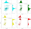 |
Fig. 1 Distribution of the confirmed exoplanets of the S1 sample in the log P – log Rp diagram for different ranges of the insulation flux. The upper left panel shows the 586 planets that receive ≤50 F⊕, the upper right panel shows the 364 planets that receive between 50 F⊕ and 200 F⊕, the lower left panel depicts the 238 planets that receive between 200 F⊕ and 550 F⊕, and the lower right panel illustrates the 339 planets with F > 550 F⊕. |
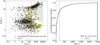 |
Fig. 2 Analysis of the planetary distribution in the F – Rp plane and the flux cumulative distribution function. Left panel: distribution of the 1527 planets of the S1 set in the F – Rp plane. The yellow triangles represent planets that would be referred to as hot Neptunes according to the limits obtained by Mazeh et al. (2016). The grey triangle is a qualitative representation of the desert. Right panel: cumulative distribution function of incident flux values F of planets with 3 R⊕ ≤ Rp ≤ 11 R⊕. The vertical dashed line in both panels represents the threshold value of 200 F⊕ below which lie 75% of the planets with 3 R⊕ ≤ Rp ≤ 11 R⊕. |
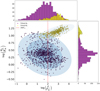 |
Fig. 3 Application of a two-component bivariate GMM over S1 sample in the log F – log Rp space. We found two separate populations: group AR (purple dots) with a mean value of (1.70,0.34), and Group BR (yellow dots) with a mean value of (2.72, 1.12). |
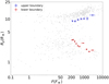 |
Fig. 4 Calculated boundaries in (F, Rp) space: (Flow,i, Rlow,i) pairs (purple points) sample the lower boundary, and (Fup,i, Rup,j) pairs (red points) mark the upper boundary. |
2.3 The sub-Jovian/Neptunian desert in the flux-mass plane
Within our initial sample, 609 planets out of 1527 also have a planetary mass estimate with ∆Mp/Mp < 30%. We refer to this set as sample S 2. We stress that the higher threshold value for ∆Mp /Mp with respect to ∆Rp /Rp was set to guarantee enough statistics in the grid-analysis step. If we had required a ∆Mp/Mp < 10%, it would have halved the S2 sample. In Fig. 5 we show the distribution of the objects belonging to the S 2 sample in the F − Mp plane. In this parameter space, we still observe a paucity of Neptunes and sub-Jupiters that receive at least ≈550 F⊕. In this case as well, only a few Hot Neptunes, defined as the objects within the boundaries of Mazeh et al. (2016), lie within the underpopulated region (see Sect. 3.2). The right panel of Fig. 5 shows that planets with 10 M⊕ ≤ Mp ≤ 200 M⊕ are common when the flux received from their host star is ≲550 F⊕. Neptunes and sub-Jupiters that experience an incident flux F ≤ 550F⊕ are three times more frequent than those with F > 550 F⊕. Therefore, in contrast to the flux-radius diagram, the vertex of the triangle (namely the 75th percentile of the incident flux distribution of planets with mass 10 M⊕ ≤ Mp ≤ 200 M⊕) here appears to be shifted towards higher incident flux (see Sect. 2.4). As done in Sect. 2.1, we confirmed all the results found by Szabó & Kálmán (2019) and Szabó et al. (2023) in the P − Mp plane, with planets in the desert likely to have a shorter period around cooler and more metal-rich stars. We also recovered their finding that the stellar mass does not play a critical role in sculpting the desert in the P − Mp diagram.
We repeated the same steps as in Sect. 2.2 considering the planetary mass in order to find the analytic expression of the two boundaries in the (F, Mp) space. We report the result of the two-component bivariate GMM in log F − log Mp space in Fig. 6. Group AM consists of a wide variety of exoplanet types spanning several orders of magnitude in incident flux (from ≈0.1 F⊕ to ≈104 F⊕) as well as a broad spectrum of masses (from ≈0.1 M⊕ to ≈8000 M⊕). We also point out that the most massive objects in group AM tend to experience low levels of incident flux. We found the mean of group AM to be located at  . On the other hand, group BM corresponds to planets that are more massive and more irradiated than those in group AM on average. We found the mean of group BM to be located at
  . It also covers a narrower flux and mass ranges, as shown by the confidence bands of the ellipsoids. However, group BM still spans two orders of magnitudes in planetary mass beyond the threshold flux of 550 F⊕, and it is not Gaussian (Shapiro-Wilk test, p < 10−6) but a skewed distribution towards more massive planets, as shown by the marginal histogram in Fig. 6.
Thus, we needed to remove extremely massive exoplanets that otherwise would lead to large spreads in the giant populations and would distort the upper boundary computation. For this reason, we discarded all the planets with a planetary mass Mp > 600 M⊕, thus resulting in a final sample composed of 512 exoplanets with a planetary mass estimate (S3 sample hereafter). The choice of using a cutoff value of 600 M⊕ was arbitrary, but is capable of guaranteeing enough statistics in each slice.
This operation does not affect the robustness of our results since we are interested in describing the low-mass edge of the group BM distribution. However, the S3 sample contains fewer than half of the objects that were contained in the initial sample we used in Sect. 2.2, so that the statistical analysis yields larger errors over the upper and lower boundary points. Similarly, the fitted parameters through DIAMONDS are more uncertain than those retrieved in Sect. 2.2. A summary of the three samples defined in this work is given in Table 1
For the boundary calculations, we only considered exoplanets that received at lest 550 F⊕. For both groups in our sample, we created a custom grid of F values spaced such that each slice contained at least 20 elements per group. As anticipated, since the sample is much less numerous in this space of parameter, we needed to choose larger slices than we defined in Sect. 2.2. For this reason, the grid used to sample group AM consisted of only three slices and that used to slice group BM contained just four slices. The two grids span the range [550 F⊕, 4000 F⊕], and the upper limit was set to ensure enough points for a statistical analysis. In this case as well, the contamination of highly irradiated sub-Jovian planets within the savanna forced us to perform a 2σ clipping for the M distribution of group AM in each slice.
In contrast with the boundary definitions given in Eqs. (3)– (4), since the planetary masses were spread over several orders of magnitudes, we defined the boundary points as points with a z-score equal to one, as suggested by the confidence ellipsoids in Fig. 6. In this case as well, the choice of the proper ɀ score was based on an a posteriori visual inspection of the points delimiting the two boundaries. However, due to the poorer statistics in each slice, more than 75% of the exoplanets in groups AM and BM were found to be above (or below) the upper (or lower) boundary.
In particular, the lower boundary point in the ith slice of the flux grid related to group AM was calculated as
 (5)
(5)
The upper boundary point in the jth slice of the flux grid related to group BM is given by
 (6)
(6)
In Fig. 7 we show the points that delimit the lower and upper boundary in the (F, Mp) space within the range [550 F⊕, 4000 F⊕].
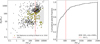 |
Fig. 5 Analysis of the planetary distribution in the F – Mp plane and the flux cumulative distribution function. Left panel: distribution of the 609 planets of the S2 set in the F – Mp plane. The yellow triangles represent planets that would be referred to as hot Neptunes according to the limits obtained by Mazeh et al. (2016). The grey triangle is a qualitative representation of the sub-Jovian and Neptune desert. Right panel: cumulative distribution function of incident flux values F of planets with 10 M⊕ ≤ Mp ≤ 200 M⊕ . The vertical dashed line represents the threshold value of 550 F⊕ in both panels below which 75% of the planets with 10M⊕ ≤ Mp ≤ 200 M⊕ lie. |
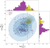 |
Fig. 6 Application of a two-component bivariate GMM on the sample S2 in the log F – log Mp space. We identified two separate populations: group AM (purple dots) with a mean value of (1.8,1.4), and group BM (yellow dots) with a mean value of (2.9, 2.5). |
Samples defined in this work and their description.
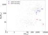 |
Fig. 7 Calculated boundaries in the (F, Mp) space: (Flow,i, Mlow,i) pairs (purple points) sample the lower boundary, and (Fup,i, Mup, j) pairs (red points) mark the upper boundary of the desert. |
2.4 About the threshold incident flux
In the F – Rp and F – Mp planes (see Sects. 2.2 and 2.3), we defined the threshold incident flux from which to start our analysis as the 75th percentile of the distribution of exoplanets with 3 R⊕ ≤ Rp ≤ 11 R⊕ and 10 M⊕ ≤ Mp ≤ 200 M⊕, respectively. We refer to this value as F75th. We found F75th ≈ 200 F⊕ in the F – Rp plane and F75th ≈ 550 F⊕ in the F – Mp plane. This raises the intriguing question whether the variation in F75th between F – Rp and F – Mp reflects an underlying physical cause, or if is it merely a consequence of the sparser data in the mass plane. In order to address the second option, we employed two different strategies: (i) We reduced the size of the S1 sample to match that of S2 and calculated F75th for planets with 3R⊕ ≤ Rp ≤ 11 R⊕, and (ii) we enlarged the size of the S 2 sample to match that of S1 and calculated F75th for planets with 10 M⊕ ≤ Mp ≤ 200 M⊕.
2.4.1 Downsizing the S1 sample
We performed 10 000 Monte Carlo simulations, in each of which the S1 sample (comprising 1527 planets) was reduced to the size of the S2 sample (609 planets) by randomly removing 918 objects. In each simulation, we calculated the F75th of exoplanets with 3 R⊕ ≤ Rp ≤ 11 R⊕ , whose distribution is shown in Fig. 8. We obtained a non-Gaussian F75th distribution with a mean value of ≈163 F⊕ and a standard deviation of ≈25 F⊕. The distribution shows a slight right-handed tail that is consistent with a skewness of ≈0.4. The non-Gaussianity was also investigated using the Anderson-Darling (AD) test (Anderson & Darling 1952), whose statistics of 65 exceeds the highest critical value by far (1.092) at the 1% significance level. The Gaussianity null hypothesis is therefore rejected at all of the provided significance levels. We opted for the AD test instead of the more commonly used Shapiro-Wilk test since the latter is known to perform better for small sample sizes (Shapiro & Wilk 1965). We found that 99.84% of our simulations yielded F75th values lower than 250 F⊕ . Moreover, only one simulations out of 10 000 returned a value of F75th ≳ 300 F⊕ , which is still much lower than the 550 F⊕ we obtained for the F – Mp diagram.
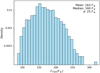 |
Fig. 8 Histogram of the variable F75th for planets with 3 R⊕ ≤ Rp ≤ 11 R⊕, generated from 10 000 Monte Carlo simulations. Each simulation reduced the S1 sample to the size of the S2 and calculated the 75th percentile of exoplanets with 3 R⊕ ≤ Rp ≤ 11 R⊕ . The histogram is normalised to show the probability density. |
2.4.2 Augmenting the S2 sample
In order to understand the effect of the small sample size on the definition of F75th and ultimately on the borders of the desert, we considered an augmented version of S2 by assigning an approximate mass estimate, derived using forecaster (Chen & Kipping 2016), to all objects in the S1 sample without a measured planetary masses. We also included in the new enlarged sample planets with ∆Mp /Mp > 30%. This procedure resulted in a S2 sample of 1527 confirmed planets, each with an estimated mass, regardless of the magnitude of the associated uncertainty. Nevertheless, even in this scenario, the F75th for planets with 10M⊕ ≤ Mp ≤ 200 M⊕ remains slightly above 400F⊕.
Thus, our statistical analysis suggests that the threshold value of the incident flux F75th is not affected by the poorer statistics in the flux-mass plane, but might be the result of a non-trivial physical effect. A similar result was obtained by Ma & Ghosh (2021): by employing a Bayesian mixture model, they found that the incident flux has a non-negligible effect on the Mp – Rp relation. Future multivariate approaches that simultaneously take into account (F, Rp, Mp) might shed light upon this issue.
2.5 The mass-radius relation
We also checked whether the GMM clustering processes performed in the two different spaces of parameters yielded any inconsistent results. In particular, one might wonder whether a planet of group AR (small radius) in the F– Rp diagram still belongs to group AM (low mass) in the F – Mp space or if it falls within the domain of group BM (high mass). If this were not the case, it would mean that planets exist whose classification depends on the physical parameter used to describe them. We performed this analysis using the S3 set of 512 exoplanets with a well-constrained planetary mass and planetary radius measurements. Our results are listed below.
We found that 271 planets (≈53% of S3 sample) are classified as belonging to group A according to both radius and mass (i.e. small radius AR and low mass AM). We term this class ARAM hereafter.
We found that 29 planets are classified as belonging to group B with respect to the radius and to group A with respect to the mass (i.e. large radius BR and low mass AM). We term this class BRAM hereafter.
We found that one planet (K2-60 b; Eigmüller et al. 2017) was classified as belonging to group A with respect to the radius and to group B with respect to the mass (i.e. small radius AR and high mass BM). We term this class ARBM hereafter.
We found that 211 planets (≈41% of S3 sample) were classified as belonging to group B for the radius and mass (i.e. large radius BR and high mass BM). We term this class BRBM hereafter.
In Fig. 9 we show the distribution of 512 objects within the log Rp – log Mp plane, each coloured according to its classification with respect to both radius and mass. It is interesting to note that the 29 planets classified as BRAM belong to the transition of the M(R) curve. The average mean planetary density of the BRAM group is ≈0.68 g/cm3 (approximately half of the mean Jupiter density) with a standard deviation of ≈0.61 g/cm3 . Thus, these objects might represent the well-known class of inflated hot Jupiters (Sestovic et al. 2018). We remark that some of the hybrid objects (i.e. belonging to groups ARBM and BRAM) might simply be the result of the precision limit of the GMM clustering. K2-60 b (Eigmüller et al. 2017) has a mean planetary density of ≈1.6g/cm3. Future spectroscopic follow-up investigations of these objects could shed light upon their proper position within the log Rp – log Mp plane.
2.6 Bayesian inference and model comparison with DIAMONDS
In order to fit the boundaries in the F – Rp plane that delimit the region of the desert, we exploited a series of different analytical models whose statistical significance was subsequently tested by means of a Bayesian model comparison process. All the fits were performed using the public Bayesian inference tool DIAMONDS3 (Corsaro & De Ridder 2014). DIAMONDS allowed us to simultaneously perform a Bayesian parameter estimation and model comparison using the nested-sampling Monte Carlo algorithm (Skilling 2004), without limitations regarding the size of the dataset or the number of free parameters involved in the model. DIAMONDS returned the Bayesian evidence (E) for each tested model. The Bayesian evidence represents the probability of the data in the light of a given model, that is, it averages the likelihood distribution over the parameter space set by the priors, namely by our choice of values of the free model parameters. In particular, E is defined as
 (7)
(7)
where θ is the parameter vector, ℒ is the likelihood, and π is the prior on the free parameters as conditional to the choice of the model ℳ, the latter defining the parameter space Σℳ over which the integral is performed. When we compare the two models M1 and ℳ2, the corresponding Bayes factor B1,2 of ℳ1 relative to ℳ2 is defined as the ratio of the model evidence, or equivalently, as ln B1,2 ≡ ln ℰ1 – ln ℰ2 when we adopt a logarithmic form. For ln B1,2 ≥ 5 (Jeffreys 1961), the evidence condition in favour of model ℳ1 is strong, meaning that this model can be considered with a probability higher than 99% to be the favoured choice.
The first model we took into account was a power-law model of the form
 (8)
(8)
with the free parameters α and β. In order to incorporate the uncertainties on the independent variable F, we linearised this model by adopting a logarithmic scale,
 (9)
(9)
This model, hereafter model  , has the free parameters (α, ln β).
As a second option, we considered the linear model
 (10)
(10)
hereafter termed model  , with (a, b) as free parameters.
We performed a Bayesian inference on the two models presented above by adopting a Gaussian likelihood that incorporated the uncertainties on the planet radii and fluxes. The corresponding log-likelihood reads
![$\Lambda (\theta ) = {\Lambda _0}(\theta ) - {1 \over 2}\mathop \sum \limits_{i = 1}^N {\left[ {{{{\Delta _i}(\theta )} \over {{{\mathop \sigma \limits^ }_i}(\theta )}}} \right]^2},$](/articles/aa/full_html/2024/12/aa51252-24/aa51252-24-eq22.png) (11)
(11)
where θ is the parameters vector (e.g. (α, ln β) for model ℳ1), N is the total number of points considered in each boundary,  is the relative uncertainty over θ, and Λ0(θ) is a term depending on the relative uncertainties, given by
 (12)
(12)
Lastly, we considered a third model, termed  , which extended the linearity to a quadratic regime, but this time, without the uncertainties in the covariates F. The model reads
 (13)
(13)
and the free parameters are  . The outputs of DIAMONDS in the flux-radius diagram are discussed in Sect. 3.1.
In addition to the investigation of the F – Rp plane, we performed a similar analysis in the F – Mp space. In particular, we analysed the analogous of models  and
and  by replacing the planet radius Rp with the planet mass Mp, from which we obtained models
  and
and  . We did not consider the quadratic model
  because too few points are available to constrain the larger number of free parameters. The outputs of DIAMONDS in the flux-mass diagram are discussed in Sect. 3.2.
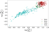 |
Fig. 9 Distribution of 512 objects of sample S3 within the log Rp – log Mp plane, coloured according to their classification with respect to the radius and mass. 271 blue dots (ARAM) represent the planets classified as not giants for the radius and mass, 211 red dots (BRBM) represent the planets labelled as giants for the radius and mass, 29 green points (BRAM) are giant planets according to their radius and not giants according to their mass, and the one yellow point (ARBM) corresponds to a not-giant in terms of the radius and to a giant with respect to the planetary mass. |
3 Results
The analysis presented in Sect. 2 shows that a paucity of highly irradiated Neptunes and sub-Jovians exists in the flux-radius and flux-mass diagrams. This feature suggests a dichotomy of planets at a high level of incident flux (≳200 F⊕): sub- Neptunes/super-Earths, and Jupiters/super-Jupiters. By using the GMM algorithm, we determined the upper and lower edges in the flux-radius and flux-mass planes as described in Sects. 2.2 and 2.3. We then fitted each edge in the two planes using DIAMONDS, as shown in Sect. 2.6. Thus, the depletion region delimited by the two boundaries here takes the orbital period of the planet and the fundamental properties of the host star into account.
3.1 Flux-radius plane
The Bayesian evidence E computed through DIAMONDS is listed in Table 2. The model that is clearly favoured for the lower and upper boundary is the power-law model  , for which the Bayes factors largely exceeds the strong-evidence condition (ln B > 5.0). We noted that the model involving a quadratic dependence upon F is subject to significant departures from the data regime for values outside the range imposed by the data. As appears evident from the reported Bayesian evidence, the larger number of free parameters of this latter model significantly penalises its statistical weight as compared to the other models that we took into account in our study (Jeffreys 1961).
In Table 3 we report the best-fitting values for α and ln β of the power-law model  as retrieved by DIAMONDS. We name the area comprised between the boundaries obtained with the
  model irradiation desert in the F – Rp plane.
In Fig. 10 we show the distribution of S1 sample in the P–Rp diagram alongside the Mazeh et al. (2016) boundaries and within the F – Rp diagram alongside the lower and upper boundaries obtained in this work. Out of 221 hot Neptunes, identified in the P – Rp diagram, 194 fall outside the irradiation desert in the F – Rp plane or lie along its edges. Future refinements of the orbital and physical parameters of the objects lying on the edges could shed light upon their membership of the desert. Only 27 out of 221 planets occupy the statistical scarcely populated region within the F – Rp diagram. Thus, according to this new perspective, the 194 planets are not so rare, even though they were earlier classified as hot Neptunes. Furthermore, we also checked whether any planet of our sample that resides outside the desert as defined by Mazeh et al. (2016) (in the P – Rp diagram) would fall inside the desert derived in this work. Only three planets satisfy this condition, and they are Kepler-1270 b ( and P = 6.03356196 ± 0.00006551 days; Morton et al. 2016), Kepler-815 b (
 and P = 8.57503552 ± 0.0000591 days) and KOI-94 c (Rp = 4.32 ± 0.41 R⊕ and P = 10.423707 ± 0.000026 days; Weiss et al. 2013; Masuda et al. 2013). As shown in Fig. 10, while these planets lie nearby but outside of the lower boundary as defined by Mazeh et al. (2016), they fall well inside the desert found in this work.
Bayesian evidence for the models defined in this work.
Parameter estimation results for the power-law models  and
and  as obtained by DIAMONDS.
3.2 Flux-Mass plane
We also fitted the two edges of the sub-Jovian and Neptune desert within the F – Mp plane using DIAMONDS. As in the previous case, the model that is clearly favoured for the lower and upper boundary is the power-law model  , and its Bayes factors largely exceeds the strong-evidence condition (ln B > 5.0), as shown in Table 2.
In Table 3 we report the best-fitting values for α and ln β of the power-law model  as retrieved by DIAMONDS. We name the area between the boundaries obtained with the
  model the irradiation desert in the F – Mp plane. With respect to the results obtained for the flux-radius plane (see Sect. 3.1), the errors on the fitted parameters are relatively larger because the statistics in the flux-mass diagram are larger, as already discussed in Sect. 2.3. Within the S3 sample, 110 planets are found to populate the desert obtained by Mazeh et al. (2016) in the P – Mp diagram. Figure 11 depicts the distribution of these planets in the F – Mp diagram, together with the lower and upper boundaries obtained in this work. As discussed in Sect. 2.3, because the statistics in the flux-mass plane are lower, the confidence bands of the edges overlap when we take the uncertainties on the fit in the flux-mass plane into account, as shown in Fig. 11. However, 63 planets out of 110 still receive an incident flux F ≤ 550 F⊕ and therefore do not populate the irradiation desert in the F – Mp plane. This might be the result of using a different F75th between the F – Rp and F – Mp planes because this effect does not clearly arise when we considered the orbital period in place of the incident flux.
In Sect. 2.4.2 we constructed an augmented version of sample S2 by using forecaster to obtain an Mp estimate for planets without mass measurements and keeping objects regardless of the magnitude of the uncertainty ∆Mp /Mp. In principle, we could have used this sample to compute the analytical expression of the lower and upper boundary in the F – Mp plane. However, even though this approach would yield a larger data set to be fitted with DIAMONDS, we definitely lose much in accuracy. Typically, the uncertainties in Mp estimated by forecaster range from approximately 30 to 50% for well-characterised exoplanets, but this can be significantly higher for planets with less precise data. In particular, for our data set, we found the uncertainties to be normally distributed around ≈60% with a standard deviation of about 5%. Consequently, even though employing an augmented sample might help us to mitigate the issues associated with limited statistics in the F – Mp plane, the results would ultimately rely on a highly uncertain sample, which would lead to unreliable boundary points.
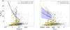 |
Fig. 10 Comparison of the S–1 sample distribution in the P – Rp and F – Rp planes to highlight the irradiation desert. Left: distribution of the S–1 sample in the P – Rp diagram along the edges obtained by Mazeh et al. (2016). The yellow triangles represent the 221 hot Neptunes within the S1 sample according to the definition of Mazeh et al. (2016) in the P – Rp plane. The black dots represent all the planets that lie outside the desert. Right: distribution of the S1 sample in the F – Rp plane. The orange and blue lines represent the lower and upper boundary obtained in Sect. 3.1 alongside their confidence bands (1σ). The yellow triangles show the 194 out of 221 objects that do not lie within the irradiation desert defined in this work. The yellow triangles used to designate the hot Neptunes in the P – Rp diagram still refer to the same planets in the right plot. The red stars indicate planets that fall within our defined boundaries but not within those outlined by Mazeh et al. (2016). |
3.3 Planetary mean density
In Sects. 3.1 and 3.2 we obtained the analytic expressions of the boundaries of the sub-Jovian and Neptune desert in the F – Rp and F – Mp planes. For each edge, by combining Rp (F) and Mp (F), we can obtain a mass-radius relation in order to understand what types of planet populate them. In particular, the mass-radius relation for the upper boundary is given by
 (14)
(14)
while the mass-radius relation describing the lower boundary is
 (15)
(15)
We show the mass-radius relations for the two boundaries in Fig. 12. Planets populating the upper edge of the sub-Jovian and Neptune desert in the F – Rp and F – Mp planes are compatible with very low planetary density values (≈0.1 g/cm3), thus suggesting a gaseous nature. The resulting exponent (0.23 ± 0.15) agrees well with the findings of Mazeh et al. (2016) within the numerical uncertainties. On the other hand, planets lying on the lower edge systematically have a higher density. The spread of the curve, which is mostly due to the uncertainty on the mass estimates, leads to a certain level of ambiguity: These planets could either be covered by a gaseous envelope that drastically reduces the mean planetary density, or they might be silicate worlds. The former case might be compatible with a low-mass planet covered by a H/He envelope that undergoes photoevaporation due to the stellar irradiation of the host. The latter might represent the final stage of the previous scenario where the planet has lost part of its envelope.
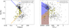 |
Fig. 11 Comparison of the S3 sample distribution in the P – Mp and F – Mp planes to highlight the irradiation desert. Left: distribution of the S3 sample in the P– Mp diagram along the edges obtained by Mazeh et al. (2016). The yellow dots represent the 110 hot Neptunes within S3 according to the definition of Mazeh et al. (2016) in the P – Mp plane. The black dots represent planets outside the desert. Right: distribution of our sample in the F – Mp plane. The orange and blue lines represent the lower and upper boundary obtained in Sect. 3.2 alongside their confidence bands (1σ). The red dots show that 63 out of 110 objects experience an incident flux lower than 550 F⊕. The yellow triangles used to designate the hot Neptunes in the P – Mp diagram still refer to the same planets in the right plot. |
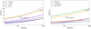 |
Fig. 12 Mass-radius relations for the upper (orange line) and lower boundary (blue line) given by Eqs. (14) and (15), respectively. We present different curves at fixed density (left). While the upper boundary is consistent with a very low mean planetary density (≈0.1 g/cm3), the lower boundary comprises different values spanning from ≈1 g/cm3 to ≈2g/cm3. We also present different mass-radius curves for different planetary compositions (right). |
4 Conclusions
We have expanded upon the seminal work of Mazeh et al. (2016) by studying the sub-Jovian and Neptune desert in more detail. This is the region of the P – Rp and P – Mp space parameters from which Neptunian exoplanets with short orbital periods are notably absent. The orbital period is not a complete physical variable for understanding the nature of this phenomenon because it does not account for stellar radiation. Our analysis therefore incorporated the incident flux from the host star in order to provide a more comprehensive picture of the factors influencing the formation and evolution of these intriguing exoplanets.
Our analysis revealed that the incident flux plays an important role in shaping the boundaries of the sub-Jovian and Neptune desert. We analysed the dependences of the upper and lower edges on the incident flux in the flux-radius and flux-mass space parameters. We employed DIAMONDS, a novel Bayesian nested-sampling tool, to infer the best models that fit the two boundaries in both planes. Even when we accounted for the incident flux, we still found a paucity of known Neptune- and Saturn-like exoplanets experiencing high-intensity levels of stellar radiation. We called the region in which they lie the irradiation desert. Moreover, ≈87% of planets in the desert defined by Mazeh et al. (2016) in the period-radius plane do not lie within the irradiation desert we defined in the flux-radius diagram. A similar result was obtained in the flux-mass plane. Thus, the sub- Jovian and Neptune desert is likely much more desolate than we would expect. We stress that our method yielded boundaries that delimit a region that admits contamination by a few moderately irradiated Neptunes and sub-Jovians.
We also retrieved the mass-radius relation for the planets lying close to the two boundaries. While the upper boundary is populated by exoplanets with a very low mean planetary density, which is compatible with gas giants that are stable against the photoevaporation scenario, the lower boundary comprises a broader range of planetary types: from planets with gaseous envelops to objects with a higher mean planetary density, which might be compatible with worlds dominated by silicates.
Future observations with advanced telescopes such as the James Webb Space Telescope (JWST, Gardner et al. 2023) and exoplanetary missions, as well as an ongoing analysis of the thousands of planet candidates that have yet to be confirmed, will help us to refine the calculations of the two boundaries and will thus allow us to potentially reveal new insights into the nature and origins of Neptune-sized exoplanets in close orbits. In particular, the PLAnetary Transits and Oscillations of stars (PLATO, Rauer et al. 2014, 2024) mission is expected to discover several hundreds to thousands of Neptune-sized exoplanets orbiting their star in fewer than 5 days, depending on the assumed planet occurrence rates (Matuszewski et al. 2023). PLATO will not only enhance our understanding of planetary architectures by expanding the exoplanetary populations, but its high-photometric precision, combined with a host star characterisation via asteroseismology, will allow us to refine the planetary and stellar parameters. This will reduce the uncertainty on the data used in this work.
As the volume of these discoveries increases, there will be a critical need for efficient vetting processes, both through human expertise and automated machine-learning techniques (e.g. McCauliff et al. 2015; Coughlin et al. 2016; Mislis et al. 2016; Shallue & Vanderburg 2018; Yu et al. 2019; Tey et al. 2023; Fiscale et al. 2023), to ensure the accuracy and reliability of confirmed planets. However, the complexity of machinelearning models, which are often perceived as black-box systems, can limit transparency and scientific understanding. Therefore, integrating explainable machine-learning methods (Maratea & Ferone 2019) into future vetting pipelines will be essential. These techniques will allow scientists to maintain control over and insight into the decision-making process, enabling greater confidence in the discoveries and fostering collaboration between computational tools and human expertise in the validation of new exoplanet candidates.
Acknowledgements
This research has made use of the NASA Exoplanet Archive, which is operated by the California Institute of Technology, under contract with the National Aeronautics and Space Administration under the Exoplanet Exploration Program. We thank the anonymous referee whose careful reading helped to improve the quality of our manuscript. E.C. acknowledges support from PLATO ASI INAF agreement no. 2022-28-HH.0 “PLATO Fase D”. G.C. thanks the University of Napoli Federico II (project: FRA-CosmoHab, CUP E65F22000050001). Software: DIAMONDS (Corsaro & De Ridder 2014), forecaster (Chen & Kipping 2016).
References
- Allart, R., Bourrier, V., Lovis, C., et al. 2018, Science, 362, 1384 [Google Scholar]
- Allart, R., Bourrier, V., Lovis, C., et al. 2019, A&A, 623, A58 [NASA ADS] [CrossRef] [EDP Sciences] [Google Scholar]
- Anderson, T. W., & Darling, D. A. 1952, Ann. Math. Stat., 23, 193 [Google Scholar]
- Armstrong, D. J., Lopez, T. A., Adibekyan, V., et al. 2020, Nature, 583, 39 [Google Scholar]
- Attia, O., Bourrier, V., Delisle, J. B., & Eggenberger, P. 2023, A&A, 674, A120 [NASA ADS] [CrossRef] [EDP Sciences] [Google Scholar]
- Beaugé, C., & Nesvorný, D. 2013, ApJ, 763, 12 [Google Scholar]
- Benítez-Llambay, P., Masset, F., & Beaugé, C. 2011, A&A, 528, A2 [NASA ADS] [CrossRef] [EDP Sciences] [Google Scholar]
- Bourrier, V., Attia, O., Mallonn, M., et al. 2023, A&A, 669, A63 [NASA ADS] [CrossRef] [EDP Sciences] [Google Scholar]
- Burt, J. A., Nielsen, L. D., Quinn, S. N., et al. 2020, AJ, 160, 153 [Google Scholar]
- Castro-González, A., Bourrier, V., Lillo-Box, J., et al. 2024, A&A, 689, A250 [NASA ADS] [CrossRef] [EDP Sciences] [Google Scholar]
- Chen, J., & Kipping, D. 2016, ApJ, 834, 17 [Google Scholar]
- Corsaro, E., & De Ridder, J. 2014, A&A, 571, A71 [NASA ADS] [CrossRef] [EDP Sciences] [Google Scholar]
- Coughlin, J. L., Mullally, F., Thompson, S. E., et al. 2016, ApJS, 224, 12 [Google Scholar]
- Davis, T. A., & Wheatley, P. J. 2009, MNRAS, 396, 1012 [CrossRef] [Google Scholar]
- Demory, B.-O., & Seager, S. 2011, ApJS, 197, 12 [NASA ADS] [CrossRef] [Google Scholar]
- Eigmüller, P., Gandolfi, D., Persson, C. M., et al. 2017, AJ, 153, 130 [CrossRef] [Google Scholar]
- Feigelson, E. D., & Babu, G. J. 2012, Modern Statistical Methods for Astronomy (Cambridge: Cambridge University Press) [Google Scholar]
- Fiscale, S., Inno, L., Ciaramella, A., et al. 2023, in Applications of Artificial Intelligence and Neural Systems to Data Science (Berlin: Springer), 127 [Google Scholar]
- Gaia Collaboration (Prusti, T., et al.) 2016, A&A, 595, A1 [NASA ADS] [CrossRef] [EDP Sciences] [Google Scholar]
- Gardner, J. P., Mather, J. C., Abbott, R., et al. 2023, PASP, 135, 068001 [NASA ADS] [CrossRef] [Google Scholar]
- Guilluy, G., Bourrier, V., Jaziri, Y., et al. 2023, A&A, 676, A130 [NASA ADS] [CrossRef] [EDP Sciences] [Google Scholar]
- Ionov, D. E., Pavlyuchenkov, Y. N., & Shematovich, V. I. 2018, MNRAS, 476, 5639 [Google Scholar]
- Ivezić, Ž., Connolly, A. J., VanderPlas, J. T., & Gray, A. 2020, Statistics, Data Mining, and Machine Learning in Astronomy. A Practical Python Guide for the Analysis of Survey Data, Updated Edition (Princeton: Princeton University Press) [Google Scholar]
- Jeffreys, H. 1961, Theory of Probability, 3rd edn. (Oxford: Oxford University Press) [Google Scholar]
- Jenkins, J. S., Díaz, M. R., Kurtovic, N. T., et al. 2020, Nat. Astron., 4, 1148 [Google Scholar]
- Kálmán, S., Szabó, G. M., Borsato, L., et al. 2023, MNRAS, 522, 488 [CrossRef] [Google Scholar]
- Laughlin, G., & Lissauer, J. J. 2015, in Treatise on Geophysics, ed. G. Schubert (Amsterdam: Elsevier), 673 [CrossRef] [Google Scholar]
- Laughlin, G., Crismani, M., & Adams, F. C. 2011, ApJ, 729, L7 [NASA ADS] [CrossRef] [Google Scholar]
- Lopez, E. D., & Fortney, J. J. 2014, ApJ, 792, 1 [Google Scholar]
- Lundkvist, M. S., Kjeldsen, H., Albrecht, S., et al. 2016, Nat. Commun., 7, 11201 [Google Scholar]
- Ma, Q., & Ghosh, S. K. 2021, MNRAS, 505, 3853 [NASA ADS] [CrossRef] [Google Scholar]
- Magliano, C., Covone, G., Dobal, R., et al. 2023a, MNRAS, 519, 1562 [Google Scholar]
- Magliano, C., Kostov, V., Cacciapuoti, L., et al. 2023b, MNRAS, 521, 3749 [CrossRef] [Google Scholar]
- Majewski, S. R., Schiavon, R. P., Frinchaboy, P. M., et al. 2017, AJ, 154, 94 [NASA ADS] [CrossRef] [Google Scholar]
- Maratea, A., & Ferone, A. 2019, in Fuzzy Logic and Applications, eds. R. Fullér, S. Giove, & F. Masulli (Cham: Springer International Publishing), 253 [CrossRef] [Google Scholar]
- Masuda, K., Hirano, T., Taruya, A., Nagasawa, M., & Suto, Y. 2013, ApJ, 778, 185 [NASA ADS] [CrossRef] [Google Scholar]
- Matsakos, T., & Königl, A. 2016, ApJ, 820, L8 [Google Scholar]
- Matuszewski, F., Nettelmann, N., Cabrera, J., Börner, A., & Rauer, H. 2023, A&A, 677, A133 [NASA ADS] [CrossRef] [EDP Sciences] [Google Scholar]
- Mazeh, T., Zucker, S., & Pont, F. 2005, MNRAS, 356, 955 [NASA ADS] [CrossRef] [Google Scholar]
- Mazeh, T., Holczer, T., & Faigler, S. 2016, A&A, 589, A75 [NASA ADS] [CrossRef] [EDP Sciences] [Google Scholar]
- McCauliff, S. D., Jenkins, J. M., Catanzarite, J., et al. 2015, ApJ, 806, 6 [NASA ADS] [CrossRef] [Google Scholar]
- McDonald, G. D., Kreidberg, L., & Lopez, E. 2019, ApJ, 876, 22 [Google Scholar]
- Melton, E. J., Feigelson, E. D., Montalto, M., et al. 2023, arXiv e-prints [arXiv:2302.06744] [Google Scholar]
- Melton, E. J., Feigelson, E. D., Montalto, M., et al. 2024a, AJ, 167, 202 [NASA ADS] [CrossRef] [Google Scholar]
- Melton, E. J., Feigelson, E. D., Montalto, M., et al. 2024b, AJ, 167, 203 [NASA ADS] [CrossRef] [Google Scholar]
- Meng, X.-L., & Van Dyk, D. 2002, J. R. Stat. Soc. Ser. B, 59, 511 [Google Scholar]
- Miller, N., & Fortney, J. J. 2011, ApJ, 736, L29 [NASA ADS] [CrossRef] [Google Scholar]
- Mislis, D., Bachelet, E., Alsubai, K. A., Bramich, D. M., & Parley, N. 2016, MNRAS, 455, 626 [CrossRef] [Google Scholar]
- Morton, T. D., Bryson, S. T., Coughlin, J. L., et al. 2016, ApJ, 822, 86 [Google Scholar]
- Murgas, F., Astudillo-Defru, N., Bonfils, X., et al. 2021, A&A, 653, A60 [NASA ADS] [CrossRef] [EDP Sciences] [Google Scholar]
- Naponiello, L., Mancini, L., Sozzetti, A., et al. 2023, Nature, 622, 255 [NASA ADS] [CrossRef] [Google Scholar]
- Nortmann, L., Pallé, E., Salz, M., et al. 2018, Science, 362, 1388 [Google Scholar]
- Oklopčić, A., & Hirata, C. M. 2018, ApJ, 855, L11 [Google Scholar]
- Owen, J. E. 2019, Ann. Rev. Earth Planet. Sci., 47, 67 [Google Scholar]
- Owen, J. E., & Lai, D. 2018, MNRAS, 479, 5012 [Google Scholar]
- Owen, J. E., & Wu, Y. 2013, ApJ, 775, 105 [Google Scholar]
- Persson, C. M., Georgieva, I. Y., Gandolfi, D., et al. 2022, A&A, 666, A184 [NASA ADS] [CrossRef] [EDP Sciences] [Google Scholar]
- Rauer, H., Catala, C., Aerts, C., et al. 2014, Exp. Astron., 38, 249 [Google Scholar]
- Rauer, H., Aerts, C., Cabrera, J., et al. 2024, arXiv e-prints [arXiv:2406.05447] [Google Scholar]
- Salz, M., Czesla, S., Schneider, P. C., et al. 2018, A&A, 620, A97 [NASA ADS] [CrossRef] [EDP Sciences] [Google Scholar]
- Sanchis-Ojeda, R., Rappaport, S., Winn, J. N., et al. 2014, ApJ, 787, 47 [Google Scholar]
- Sestovic, M., Demory, B.-O., & Queloz, D. 2018, A&A, 616, A76 [NASA ADS] [CrossRef] [EDP Sciences] [Google Scholar]
- Shallue, C. J., & Vanderburg, A. 2018, AJ, 155, 94 [NASA ADS] [CrossRef] [Google Scholar]
- Shapiro, S. S., & Wilk, M. B. 1965, Biometrika, 52, 591 [Google Scholar]
- Skilling, J. 2004, AIP Conf. Proc., 735, 395 [Google Scholar]
- Smith, A. M. S., Acton, J. S., Anderson, D. R., et al. 2021, A&A, 646, A183 [NASA ADS] [CrossRef] [EDP Sciences] [Google Scholar]
- Szabó, G. M., & Kálmán, S. 2019, MNRAS, 485, L116 [Google Scholar]
- Szabó, G. M., & Kiss, L. L. 2011, ApJ, 727, L44 [Google Scholar]
- Szabó, G. M., Kálmán, S., Borsato, L., et al. 2023, A&A, 671, A132 [NASA ADS] [CrossRef] [EDP Sciences] [Google Scholar]
- Tey, E., Moldovan, D., Kunimoto, M., et al. 2023, AJ, 165, 95 [NASA ADS] [CrossRef] [Google Scholar]
- Thorngren, D. P., & Fortney, J. J. 2018, AJ, 155, 214 [Google Scholar]
- Thorngren, D. P., Lee, E. J., & Lopez, E. D. 2023, ApJ, 945, L36 [NASA ADS] [CrossRef] [Google Scholar]
- Vissapragada, S., Knutson, H. A., Greklek-McKeon, M., et al. 2022, AJ, 164, 234 [NASA ADS] [CrossRef] [Google Scholar]
- Weiss, L. M., Marcy, G. W., Rowe, J. F., et al. 2013, ApJ, 768, 14 [Google Scholar]
- West, R. G., Gillen, E., Bayliss, D., et al. 2019, MNRAS, 486, 5094 [Google Scholar]
- Yu, L., Vanderburg, A., Huang, C., et al. 2019, AJ, 158, 25 [NASA ADS] [CrossRef] [Google Scholar]
- Zasowski, G., Cohen, R. E., Chojnowski, S. D., et al. 2017, AJ, 154, 198 [Google Scholar]
All Tables
Parameter estimation results for the power-law models and as obtained by DIAMONDS.
All Figures
|
Fig. 1 Distribution of the confirmed exoplanets of the S1 sample in the log P – log Rp diagram for different ranges of the insulation flux. The upper left panel shows the 586 planets that receive ≤50 F⊕, the upper right panel shows the 364 planets that receive between 50 F⊕ and 200 F⊕, the lower left panel depicts the 238 planets that receive between 200 F⊕ and 550 F⊕, and the lower right panel illustrates the 339 planets with F > 550 F⊕. |
| In the text | |
|
Fig. 2 Analysis of the planetary distribution in the F – Rp plane and the flux cumulative distribution function. Left panel: distribution of the 1527 planets of the S1 set in the F – Rp plane. The yellow triangles represent planets that would be referred to as hot Neptunes according to the limits obtained by Mazeh et al. (2016). The grey triangle is a qualitative representation of the desert. Right panel: cumulative distribution function of incident flux values F of planets with 3 R⊕ ≤ Rp ≤ 11 R⊕. The vertical dashed line in both panels represents the threshold value of 200 F⊕ below which lie 75% of the planets with 3 R⊕ ≤ Rp ≤ 11 R⊕. |
| In the text | |
|
Fig. 3 Application of a two-component bivariate GMM over S1 sample in the log F – log Rp space. We found two separate populations: group AR (purple dots) with a mean value of (1.70,0.34), and Group BR (yellow dots) with a mean value of (2.72, 1.12). |
| In the text | |
|
Fig. 4 Calculated boundaries in (F, Rp) space: (Flow,i, Rlow,i) pairs (purple points) sample the lower boundary, and (Fup,i, Rup,j) pairs (red points) mark the upper boundary. |
| In the text | |
|
Fig. 5 Analysis of the planetary distribution in the F – Mp plane and the flux cumulative distribution function. Left panel: distribution of the 609 planets of the S2 set in the F – Mp plane. The yellow triangles represent planets that would be referred to as hot Neptunes according to the limits obtained by Mazeh et al. (2016). The grey triangle is a qualitative representation of the sub-Jovian and Neptune desert. Right panel: cumulative distribution function of incident flux values F of planets with 10 M⊕ ≤ Mp ≤ 200 M⊕ . The vertical dashed line represents the threshold value of 550 F⊕ in both panels below which 75% of the planets with 10M⊕ ≤ Mp ≤ 200 M⊕ lie. |
| In the text | |
|
Fig. 6 Application of a two-component bivariate GMM on the sample S2 in the log F – log Mp space. We identified two separate populations: group AM (purple dots) with a mean value of (1.8,1.4), and group BM (yellow dots) with a mean value of (2.9, 2.5). |
| In the text | |
|
Fig. 7 Calculated boundaries in the (F, Mp) space: (Flow,i, Mlow,i) pairs (purple points) sample the lower boundary, and (Fup,i, Mup, j) pairs (red points) mark the upper boundary of the desert. |
| In the text | |
|
Fig. 8 Histogram of the variable F75th for planets with 3 R⊕ ≤ Rp ≤ 11 R⊕, generated from 10 000 Monte Carlo simulations. Each simulation reduced the S1 sample to the size of the S2 and calculated the 75th percentile of exoplanets with 3 R⊕ ≤ Rp ≤ 11 R⊕ . The histogram is normalised to show the probability density. |
| In the text | |
|
Fig. 9 Distribution of 512 objects of sample S3 within the log Rp – log Mp plane, coloured according to their classification with respect to the radius and mass. 271 blue dots (ARAM) represent the planets classified as not giants for the radius and mass, 211 red dots (BRBM) represent the planets labelled as giants for the radius and mass, 29 green points (BRAM) are giant planets according to their radius and not giants according to their mass, and the one yellow point (ARBM) corresponds to a not-giant in terms of the radius and to a giant with respect to the planetary mass. |
| In the text | |
|
Fig. 10 Comparison of the S–1 sample distribution in the P – Rp and F – Rp planes to highlight the irradiation desert. Left: distribution of the S–1 sample in the P – Rp diagram along the edges obtained by Mazeh et al. (2016). The yellow triangles represent the 221 hot Neptunes within the S1 sample according to the definition of Mazeh et al. (2016) in the P – Rp plane. The black dots represent all the planets that lie outside the desert. Right: distribution of the S1 sample in the F – Rp plane. The orange and blue lines represent the lower and upper boundary obtained in Sect. 3.1 alongside their confidence bands (1σ). The yellow triangles show the 194 out of 221 objects that do not lie within the irradiation desert defined in this work. The yellow triangles used to designate the hot Neptunes in the P – Rp diagram still refer to the same planets in the right plot. The red stars indicate planets that fall within our defined boundaries but not within those outlined by Mazeh et al. (2016). |
| In the text | |
|
Fig. 11 Comparison of the S3 sample distribution in the P – Mp and F – Mp planes to highlight the irradiation desert. Left: distribution of the S3 sample in the P– Mp diagram along the edges obtained by Mazeh et al. (2016). The yellow dots represent the 110 hot Neptunes within S3 according to the definition of Mazeh et al. (2016) in the P – Mp plane. The black dots represent planets outside the desert. Right: distribution of our sample in the F – Mp plane. The orange and blue lines represent the lower and upper boundary obtained in Sect. 3.2 alongside their confidence bands (1σ). The red dots show that 63 out of 110 objects experience an incident flux lower than 550 F⊕. The yellow triangles used to designate the hot Neptunes in the P – Mp diagram still refer to the same planets in the right plot. |
| In the text | |
|
Fig. 12 Mass-radius relations for the upper (orange line) and lower boundary (blue line) given by Eqs. (14) and (15), respectively. We present different curves at fixed density (left). While the upper boundary is consistent with a very low mean planetary density (≈0.1 g/cm3), the lower boundary comprises different values spanning from ≈1 g/cm3 to ≈2g/cm3. We also present different mass-radius curves for different planetary compositions (right). |
| In the text | |
Current usage metrics show cumulative count of Article Views (full-text article views including HTML views, PDF and ePub downloads, according to the available data) and Abstracts Views on Vision4Press platform.
Data correspond to usage on the plateform after 2015. The current usage metrics is available 48-96 hours after online publication and is updated daily on week days.
Initial download of the metrics may take a while.