| Issue |
A&A
Volume 689, September 2024
|
|
|---|---|---|
| Article Number | A55 | |
| Number of page(s) | 12 | |
| Section | Planets and planetary systems | |
| DOI | https://doi.org/10.1051/0004-6361/202450552 | |
| Published online | 02 September 2024 | |
An investigation into Venusian atmospheric chemistry based on an open-access photochemistry-transport model at 0–112 km
1
College of Meteorology and Oceanography, National University of Defense Technology,
Changsha,
China
e-mail: This email address is being protected from spambots. You need JavaScript enabled to view it.
; This email address is being protected from spambots. You need JavaScript enabled to view it.
2
National Space Institute, Technical University of Denmark,
Lyngby,
Denmark
Received:
29
April
2024
Accepted:
1
July
2024
Abstract
Atmospheric chemistry plays a crucial role in the evolution of climate habitability on Venus. It has been widely explored by chemistry-transport models, but some characteristics are still poorly interpreted. This study is devoted to developing an open-access chemistry-transport model spanning both the middle and lower atmospheres of Venus. It provides a scheme for the structure of the chemistry, especially for the sulfur and oxygen, and investigates the influence of the cloud diffusivity and the SO2 dissolution that are adopted in the clouds. The developed model is based on the VULCAN framework and was updated with the state-of-the-art Venusian atmospheric chemistry. It includes vertical eddy diffusion retrieved recently with the Venus Express observations, and it resolves radiative transfer containing gas absorption and scattering, Mie scattering of the cloud droplets, and absorption of the unknown UV absorber. The obtained abundance profiles of SO, SO2, CO, COS, O, O2, O3, HCl, and NO are in overall agreement with the observations. The results show that the increase in cloud diffusivity has slight effects on the chemical structure. The SO2 mainly dissolves in 50–90 km and evaporates below the clouds. The rapid dissolution-release cycle is responsible for the large upward flux of SO2 at 58 km. At around 70 km, SO has a significant peak that is larger than that of previous studies by an order of magnitude, and S and SO2 also show slight increases. They are attributed to the buffering effects of liquid SO2 in the clouds. O2 is significantly eliminated by SO in this layer. We emphasize the superior regulation of the sulfur cycle on O2 at 70 km and its potential contributions to the long-standing problem of the overestimated O2 abundance.
Key words: planets and satellites: atmospheres / planets and satellites: individual: Venus
© The Authors 2024
 Open Access article, published by EDP Sciences, under the terms of the Creative Commons Attribution License (https://creativecommons.org/licenses/by/4.0), which permits unrestricted use, distribution, and reproduction in any medium, provided the original work is properly cited.
This article is published in open access under the Subscribe to Open model. This email address is being protected from spambots. You need JavaScript enabled to view it. to support open access publication.
1 Introduction
Venus is covered by a thick layer of atmosphere, which has a surface pressure that is about 100 times higher than that of Earth (Esposito et al. 1983). The surface temperature reaches 700 K (Seiff et al. 1985). Both features indicate that the chemical processes in the Venusian atmosphere are complicated yet efficient. Multiple studies have demonstrated a strong correlation between the atmospheric chemistry of Venus and the evolution of climate habitability. The thick clouds on Venus are mainly composed of concentrated sulfuric acid (Knollenberg & Hunten 1980; Krasnopolsky 1985), which originates from the upward transport of SO2 from the lower atmosphere and subsequent (photo)chemical reactions at the cloud top (Yung & Demore 1982; Bierson & Zhang 2020). The presence of the clouds plays a crucial role in controlling the climate by affecting the atmospheric radiative balance via their high albedo and large infrared opacity (Tomasko et al. 1980; Esposito et al. 1983; Arney et al. 2014; Titov et al. 2018). SO2 is observed to deplete in the upper clouds (Vandaele et al. 2017), which cannot be interpreted by cloud formation, as H2O is insufficient. Studies suggest that the phenomenon can be attributed to the suppression of transport within the clouds (Bierson & Zhang 2020), the dissolution of SO2 in the clouds (Rimmer et al. 2021), or even the biological activities (Schulze-Makuch et al. 2004). Observations indicate that the D/H ratio on Venus is over 100 times higher than that on Earth (de Bergh et al. 1991; Bjoraker et al. 1992; Bertaux et al. 2007; Fedorova et al. 2008), indicating the presence of a substantial initial water reservoir and significant hydrogen escape (Donahue 1999). Volcanic activities, as recently observed by Herrick & Hensley (2023), have the capacity to emit abundant SO2, H2S, H2O, CH4, and other gases that could potentially have a great impact on the atmospheric chemistry.
The photochemistry-transport model is an effective tool for comprehending the structure of planetary atmospheric chemistry. With the gradual development of Venusian exploration missions in recent decades, including Pioneer Venus (Oyama et al. 1980; Hoffman et al. 1980; von Zahn et al. 1983), Venus Express (Bertaux et al. 2007; Marcq et al. 2008; Tsang et al. 2009; Mahieux et al. 2023b,a), Akatsuki (Imamura et al. 2017), ground-based detections (Pollack et al. 1993; Arney et al. 2014; Encrenaz et al. 2020), and so on, the abundance distributions of the crucial gases such as CO, H2O, SO, SO2, H2SO4, HCl, and COS are subsequently available. These greatly facilitate the development and validation of photochemistry-transport models on Venus.
Early Venusian photochemistry-transport-model studies (Krasnopolsky & Parshev 1981; Yung & Demore 1982; Mills 1998) mainly focus on the middle atmosphere, where the photochemistry is the dominant process. In recent years, Zhang et al. (2012) and Krasnopolsky (2012) made improvements to the model parameters by incorporating the most up-to-date observations and experimental data. As a result, they developed state-of-the-art photochemistry-transport models in this region. Besides, Krasnopolsky (2007, 2013) conducted a series of studies on the thermochemical equilibrium of Venusian lower atmosphere. The aforementioned models set either the top or bottom boundaries at the cloud altitudes in order to avoid the potential issues associated with the complicated clouds. Nevertheless, the species may exhibit significant disparities in the cloud altitudes, particularly in relation to SO2 and H2O. The boundary abundances of these two species at cloud altitudes have a significant influence on their distributions in the middle atmosphere, as suggested by various model studies (Parkinson et al. 2015; Shao et al. 2020). Stolzenbach et al. (2023) developed the first 3D chemistry-transport planetary-climate Model, which includes state-of-the-art but reduced chemical networks and simplified cloud formation. By collecting the results of different model studies in the middle and lower atmospheres, Bierson & Zhang (2020) discovered that various species, particularly SOx, exhibited significant inconsistencies at the boundary altitude within the clouds. Thus, it is essential to develop a comprehensive photochemistry-transport that covers both the middle and lower atmospheres of Venus. Bierson & Zhang (2020) constructed the first one that extends from 0 to 112 km. However, their model interprets the SO2 depletion by assuming that cloud transport is suppressed, which contradicts the observed low static stability in the clouds (Imamura et al. 2017; Ando et al. 2020). Subsequently, Rimmer et al. (2021) proposed the scenario of interpreting the depletion by SO2 dissolution in the clouds, based on their developed photochemistry-transport model. However, their requirement for abundant hydroxide salts in the cloud altitudes is partly controversial. Furthermore, it is worth noting that none of the aforementioned models are available as open-access resources. There are still constraints that hinder further investigations into the atmospheric chemistry of Venus.
This study aims to fulfil three main objectives: (a) to develop an open-access chemistry-transport model spanning both the middle and lower atmospheres of Venus, using updated parameters and coefficients for the background atmospheres and reactions; (b) to provide an evaluation on the eddy diffusivity in the Venusian clouds that spans a wide range in previous studies; and (c) to deeply investigate the structure of Venusian atmospheric chemistry, especially for the role that the sulfur cycle plays in the presence of SO2 dissolution or release processes. The model description is in Sect. 2. The findings obtained from various scenarios, along with our discussions, are described in Sect. 3. Finally, we detail the conclusion of the study in Sect. 4.
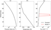 |
Fig. 1 (a) Pressure, (b) temperature, and (c) eddy diffusion coefficient profiles adopted in this study. The pressure and temperature profiles are adopted from Seiff et al. (1985). The nominal Kzz profile is adopted from Bierson & Zhang (2020). The red line in panel (c) is the global-mean Kzz profile adopted from Dai et al. (2023), which is tested in our Model A. |
2 Model description
Our global-mean atmospheric photochemical model is based on a 1D framework named VULCAN, which is commonly used on the exoplanets (Tsai et al. 2017, 2021, 2023). The model solves the continuity equations of involved species with their chemical kinetics and eddy diffusion as functions of time and altitude:
 (1)
(1)
where the footnote i represents the index of the species, the footnote atm represents the background atmosphere, n is the number density, t is the time, z is the altitude, and P and L represent the chemical production and loss rates, respectively. Kzz represents the eddy diffusion coefficient (discussed later) and Xi = ni/natm is the volume mixing ratio (VMR) of the species.
This model extends from the surface to 112 km, covering the lower and the majority of the middle atmosphere of Venus. The vertical resolution is 2 km. Since our domain is significantly lower than the homopause region (near 130 km), the species are assumed to be mixed by eddy motions, while molecular diffusion is disregarded. In addition, this upper boundary of 112 km enables us to neglect the ion chemistry. The specific ordinary differential equations (ODEs) can be found in Tsai et al. (2017, 2021).
2.1 Background atmosphere
Venus possesses a harsh surface environment characterized by elevated temperatures and pressures, resulting in a distinct lack of habitability compared to Earth. The atmospheric temperature and pressure profiles used in our model are adopted from the Venus international reference atmosphere (Seiff et al. 1985), as depicted in Fig. 1.
The atmosphere is assumed to be mixed by vertical eddy diffusion, which incorporates turbulence, convection, wave-induced processes, and so on. The efficiency of this mixing process is characterized by the eddy diffusion coefficient (Kzz, Fig. 1). The value of Kzz in our nominal model is adopted from Bierson & Zhang (2020). It slightly grows from 1.7×104 cm2 s−1 at the surface to 5.3×104 cm2 s−1 at 80 km. Then, a breakpoint appears where the Kzz starts to rapidly increase with altitude due to the additional contribution of the subsolar–antisolar circulation (Zhang et al. 2012). The values are constrained by the observations of Pioneer Venus (Woo & Ishimaru 1981; Woo et al. 1982; Lane & Opstbaum 1983). We note that the Kzz in the Venu-sian clouds is controversial due to the absence of observational constraints. Bierson & Zhang (2020) assumed a ‘Cloud Kzz’ with a value of 1×103 cm2 s−1 at 45-65 km to suppress the upward diffusion of SO2, while this seems to contradict the observed low static stability in the clouds reported by Akatsuki and Venus Express (Imamura et al. 2017; Ando et al. 2020). Lefèvre et al. (2022) retrieved the cloud Kzz by a convection-resolving model with a value exceeding 1×107 cm2 s−1. A recent study based on Venus Express observations proposed that the Kzz significantly increases in the Venusian cloud regions, even reaching 1×108 cm2 s−1 (Dai et al. 2023). In order to analyze the effect of the Kzz on the chemical structure, we adopted the global-mean Kzz profile from Dai et al. (2023) at 46.5-55 km in Model A, as opposed to the nominal model.
2.2 Atmospheric chemistry
We implemented 362 neutral chemical reactions and 45 photolysis reactions for 59 species written as follows: O, O(1D), O2, O2(1Δ), N2, CO2, H2O, CO, O3, H, HO2, OH, H2, H2O2, Cl, ClO, HCl, HOCl, Cl2, COCl, COS, SCl, ClS2, ClSO2, COCl2, OSCl, SO, SO2, SO2(l), SO3, OCO3, HSO3, H2SO4, H2SO4(l), SCl2, S, S2, S3, S2O, S4, S5, S6, S7, S8, S2O2, S2Cl2, N, NO, HNO, N2O, NO2, HNO2, NO3, HNO3, SNO, SH, H2S, SO2Cl2, and HSCl. Among them, the N2 VMR is fixed at 3.4%. H2SO4, H2SO4(l), and H2O mixing-ratio profiles are fixed, as the model does not account for the formation of sulfuric acid clouds. The two gas profiles are adopted from Bierson & Zhang (2020). The H2SO4(l) profile is adopted from Rimmer et al. (2021) to calculate the dissolution of SO2 (illustrated in Fig. 2).
The neutral reactions and their rate coefficients are collected on Zenodo (https://doi.org/1S.5281/zenodo.12696879). The network is mainly adopted from Mills (1998) in the middle atmosphere and Krasnopolsky (2007) in the lower atmosphere. In addition, we incorporate the adjustments by Zhang et al. (2012) and Bierson & Zhang (2020) on the equilibrium constants of S2O2, Sx, COCl, and the consumption pathways of COS. VULCAN has the ability to automatically calculate the reverse reaction rate based on the thermodynamic properties of the forward reactants. However, due to the large uncertainty in the experimental data of sulfur-bearing gases, we relied on existing experimental measurements and model evaluations to determine the rate coefficients for both the forward and reverse reactions. The species named by M participating in several reactions refers to the total density that is mainly contributed by CO2 and N2, acting as catalysts to increase the probability of reactant collisions.
A notable depletion of SO2 is exhibited by observations in the upper clouds, for which a comprehensive explanation is currently lacking (Vandaele et al. 2017). Hypotheses regarding either low Kzz in the clouds (Bierson & Zhang 2020) or the dissolution of SO2 in the droplets (Rimmer et al. 2021) have been proposed in the latest studies. The former is less likely as the observed static stability decreases in the clouds (Ando et al. 2015; Imamura et al. 2017), and a recent study evaluated a much higher cloud Kzz (Dai et al. 2023). Thus, in order to match the SO2 measurements, we incorporated the SO2 dissolution in the clouds in our nominal model as described by Rimmer et al. (2021):
R293 SO2 + H2SO4(l) → SO2(l) + H2SO4(l)
R294 SO2(l) + H2SO4(l) → SO2 + H2SO4(l)
R295 SO2(l) + H2SO4 → SO2 + H2SO4.
The reactions R293 and R294 refer to the dissolution of SO2 in the clouds and the release of SO2 from the droplet surface, respectively. The reaction R295 mainly contributes to the release of SO2 when the droplet rains out and evaporates below the cloud base. We note that the above reactions demonstrate the final dissolution and release processes that incorporate complicated intermediate chemistry. The rate constants are determined through empirical calculations involving Henry’s law by Rimmer et al. (2021), rather than laboratory measurements. For comparison, we outline a sensitivity test for the SO2 dissolution rate in Sect. 4.
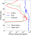 |
Fig. 2 H2SO4 (red) and H2O (blue) profiles adopted from Bierson & Zhang (2020), and liquid H2SO4 (green) profile adopted from Rimmer et al. (2021). Observations are presented for comparison. |
2.3 Radiative transfer
The radiation field ranging from 100 to 700 nm is discretized into bins with widths of 0.1 nm (<240 nm) and 2 nm (>240 nm). The incident spectral actinic flux at our upper boundary is applied directly from Zhang et al. (2012). The extinction mechanisms of the solar radiation in this model involve the absorption and scattering of the gases, the Mie scattering of the cloud droplets, and the absorption of the unknown UV absorber (Crisp 1986). The gas extinction is calculated as
 (2)
(2)
where τgas is the optical depth of the gases, σa,i and σs,i represent the cross sections of absorption and scattering for species i, respectively, and ni is the number density. In this model, the cross-sections of CO2 , H2O, and H2O2 are dependent on the temperature as suggested by Mills (1998) and Zhang et al. (2012). Cross-section data are adopted from either the Leiden Observatory database (Heays et al. 2017) or the Calt/JPL kinetics model (Zhang et al. 2012). The species contributing to Rayleigh scattering are the dominant gases CO2 , N2 , and the minor species H2 and O2, as suggested by Mills (1998).
The extinction caused by Mie scattering across a cluster of particles with varying sizes can be calculated by
 (3)
(3)
 (4)
(4)
where β represents the extinction coefficient, τp represents the part of optical depth contributed by Mie scattering from the top to altitude z, σp is the extinction cross-section, n(dp) is the number density of the particles with a diameter of dp , and Qp represents the extinction efficiency of the single particle that is dependent on the refractive index, wavelength, and particle diameter. The Qp is calculated with the latest Mie computational package PyMieScatt (Sumlin et al. 2018), which has advantages in calculating regions where valid solutions may exist within the error bounds of laboratory measurements and is convenient for interacting with this model compiled by Python. The results are then scaled to match the optical depth derived by Crisp (1986) (see their Table 2). In this model, the particle distribution is simplified by considering two modes: mode 1 (dp = 0.98 µm) and mode 2 (dp = 2.36 µm) – as demonstrated by Zhang et al. (2012) in their Figure A3 – which are based on the observations of Venus Express (above 72 km, Wilquet et al. 2009) and Pioneer Venus (58–65 km, Knollenberg & Hunten 1980). The refractive index of mode 1 is 1.45, and that of mode 2 is 1.44. Since the cloud formation is currently not released in this model, we converted the aerosol optical depth into the fit cross-sections of two modes for improving computing efficiency.
The effect of the UV absorber is also accounted for. The UV absorber is mainly concentrated in the upper clouds (Titov et al. 2018). Its composition remains unknown. A recent experimental study proposed that a specific proportion of rhomboclase [(H5O2)Fe(SO4)23H2O] and acid ferric sulfate [(H3O)Fe(SO4)2] in the concentrated sulfuric acid solution has similar optical properties to the unknown UV absorber (Jiang et al. 2024). However, their materials are formed according to a particular experimental setting, rather than a Venus-like environment. As suggested by Crisp (1986) and Zhang et al. (2012), the absorption of the UV absorber in 320–560 nm is introduced by using the absorption of the mode 1 particles in the model.
The actinic flux is then derived by
 (5)
(5)
where Jtop represents the incident spectral actinic fluxes at the top of our domain, λ is the wavelength, τ represents the total optical depth, and θ is the zenith angle of the incident beam (58°for the dayside average). The last term, Jdiff, represents the diffusive flux defined by integrating the diffuse specific intensity in all directions. It is solved by the two-stream approximation (Malik et al. 2019) and converted to total intensity by the first Eddington coefficient (Heng et al. 2018), based on the treatment of Tsai et al. (2021). The photolysis rate coefficient for gases is derived by
 (6)
(6)
where q(λ) is the quantum yield. We halved the photolysis rates to account for the diurnal average of solar flux.
Boundary conditions.
2.4 Boundary conditions
The boundary conditions are collected in Table 1. At the upper boundary, CO2 has an upper flux of 5.03×1011 cm−2 s−1. As the dominant species CO2 is photolyzed above the top of our domain, CO is produced and transported downward with the same flux of −5.03×1011 cm−2 s−1 at the upper boundary for conservation. HCl and Cl have a similar pattern with fluxes of ±1×107 cm−2 s−1. Besides this, O2 and O2(1Δ) have upward fluxes of 9×108 cm−2 s−1 and 3×108 cm−2 s−1, respectively, to account for their photolysis above. The flux of O refers to the sum of the column photolysis of CO2, O2, and O2(1Δ) above 112 km. At the bottom boundary, several species have fixed VMRs as suggested by Bierson & Zhang (2020). The H2 and H2S boundary VMRs meet the upper limits derived by Pioneer Venus (Oyama et al. 1980). Species that have not been presented are assumed to have zero fluxes at the boundaries.
3 Results
In this section, we present an overview of the species’ abundance distributions and the benchmarks.
3.1 Sulfur species
The derived mixing-ratio profiles of SO, SO2, SO3 and S2O2 are presented in Fig. 3. The SO2 mixing-ratio profile agrees with the observations of Venus Express (Marcq et al. 2008; Belyaev et al. 2014, 2012; Mahieux et al. 2015a), Pioneer Venus (Oyama et al. 1979, 1980; Hoffman et al. 1980), VeGa 1 and 2 (Bertaux et al. 1996), and ground-based remote sensings (Encrenaz et al. 2013; Krasnopolsky 2010b; Pollack et al. 1993; Bézard et al. 1993). Its VMR rapidly decreases as altitude increases between 55 and 60 km. The inverse gradient of SO2 observed by SPICAV/VEX (Belyaev et al. 2012) at 85–100 km is not retrieved in our results, which might be not purely pho- tochemically driven; there may be an unknown source of SO2 (e.g. H2SO4 and Sx aerosols that proposed by Zhang et al. 2012). Our derived SO2 abundance is significantly larger than that in Rimmer et al. (2021) above 90 km where their profile rapidly decreases with increasing altitude, contradicting the observed trends. This may be attributed to their overestimated photolysis rates of SO2 and SO as their atom S has an abnormally high abundance in this region. A similar pattern also appears in the abundances of SO and S2O2.
The SO VMR in our nominal model decreases as the altitude decreases from the top boundary, agreeing with the observations at 70–100 km derived from Venus Express (Belyaev et al. 2012; Jessup et al. 2015) and ground-based detections (Sandor et al. 2010; Encrenaz et al. 2015). The distribution pattern of S2O2 is similar to that of SO. Its VMR reaches only about 1×10⁻⁸ ppmv at 70 km and less than 1× 10⁻²¹ ppmv in the lower atmosphere. Frandsen et al. (2016) proposed that it has a similar absorption (320–400 nm) to the unknown UV absorber in the upper clouds. Krasnopolsky & Pollack (1994) suggested that S2O2 contributes to the destruction of COS in the lower atmosphere. However, the limited presence of this species is insufficient to support its candidacy as the UV absorber, and it does not deplete the abundant COS. In addition, the different treatments of the reaction between COS and S2O2 lead to the different abundances of SO and S2O2 below 50 km between this study and Rimmer et al. (2021). Although the photolysis of S2O2 into SO2 and S is addressed in Krasnopolsky (2012), there is currently no laboratory data for this process. Thus, its photolysis was not considered in this study.
The SO3 VMR peaks at 40 km as a result of the thermal decomposition of H2SO4. This is consistent with model results of Bierson & Zhang (2020) and Krasnopolsky (2007). It is also produced by the combination of SO2 and O near 70 km, which is a crucial step in cloud formation. Prior to diffusing, the generated SO3 promptly reacts with H2O to produce H2 SO4, which subsequently enters the cloud droplets through a binary condensation process facilitated by the presence of H2O (Dai et al. 2022a,b).
Figure 4 shows the distributions of additional sulfur species in the nominal model. We note that most of these species lack observational constraints. In our simulation, COS could be another reservoir of sulfur in the lower atmosphere with a VMR of 10–30 ppm. It is rapidly depleted at 40 km. Free sulfur may be mainly composed of S2 in the lower atmosphere. It has a VMR of 0.5 ppmv near the surface, in comparison to 0.75 ppmv in Krasnopolsky (2007), 0.1 ppmv in Krasnopolsky & Parshev (1980), and 0.2 ppmv in Fegley et al. (1997). Although sulfur species could have complicated chemical interactions with Cl, most of the S-Cl species on Venus are predicted to have fairly low abundances throughout our domain. Therefore, they are not described in detail in this study.
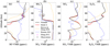 |
Fig. 3 VMR profiles of (a) SO, (b) SO2, (c) SO3, and (d) S2O2 in our cases. We note that the nominal results overlap with Model A at most altitudes. The observations (gray), the results from Bierson & Zhang (2020, orange), Rimmer et al. (2021, blue) and Zhang et al. (2012, pink) are also presented for benchmarking purposes. |
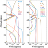 |
Fig. 4 VMR profiles of some other sulfur species in the nominal model. |
3.2 CO and COS
CO2 is the primary component of the Venusian atmosphere, which has a VMR of about 96% at the surface. Its photolysis in the middle and upper atmospheres produces abundant CO and O (Marcq et al. 2018). As the recombination of these two species is slow, they diffuse downward and the VMRs are consequently expected to decrease with decreasing altitudes.
The derived CO profiles in our study are presented in Figure 5. The results basically agree with the observations below 90 km (Bézard et al. 1990; Marcq et al. 2006, 2008, 2015, 2023; Tsang et al. 2009; Young 1972; Krasnopolsky 2010a; Oyama et al. 1980; Cotton et al. 2012; Bézard & de Bergh 2007; Mahieux et al. 2023b), but they are larger than the observations near 100 km (Krasnopolsky 2014; Mahieux et al. 2023b) by a factor of ~2. The CO VMR significantly decreases as altitude decreases from the upper boundary to 75 km. In this region, the production of CO is regulated by the photolysis of CO2, while its removal is mainly caused by its reaction with OH. The column rate of the CO2 photolysis is 2×1012 cm−2 s−1 in our nominal model, which is half of the result in Krasnopolsky (2012). CO exhibits a moderate decline below 75 km, with a VMR of 15–30 ppm.
Conversely, the COS VMR generally decreases with increasing altitude, especially at 30–40 km where the depletion of COS has the same range as the increase of CO. This is consistent with the observations (Pollack et al. 1993; Marcq et al. 2008; Krasnopolsky 2010b) and the reviews by Marcq et al. (2018). We note that the pathway of the conversion from COS to CO remains controversial in model studies. Traditional schemes involving the reactions of COS with Sx, SO3 , or S2O2 are insufficient for the complete removal of COS and fail to explain the observations at40 km (Krasnopolsky 2007, 2013; Yung et al. 2009). Several studies (Krasnopolsky & Pollack 1994; Yung et al. 2009) have suggested that an additional chemical sink beyond photolysis that converts COS to CO was required at this layer. A recent model study of Bierson & Zhang (2020) indicated a new pathway R297 COS + 2SO3 → 3SO2 + CO, with an experiential coefficient k = 3×10⁻³². Their result shows a perfect agreement with observations, and, thus, this reaction was adopted in our study. In this case, the COS abundance above 40 km deeply depends on the fixed H2SO4 abundance below the clouds, which produces SO3 by thermal decomposition.
Based on our model prediction, COS is mainly consumed by SO3 at 30–50 km. The depleting rate reaches 1×107 cm−3 s−1 at 37 km. The column rate of this process within 30–50 km is -4.78×1013 cm−2 s−1. Due to insufficient chemical production, the COS needs to rapidly diffuse upward from lower altitudes, resulting in a distinct gradient in its profile. Besides this, the net column rate of COS at 0–30 km is −1.1×1012 cm−2 s−1. This indicates that a significant source of COS is needed at the surface.
3.3 Ox, Cl and N species
The derived profiles of O, O2, O3 , OH, HCl, Cl, COCl, and ClCO3 are displayed in Fig. 6. The O profile in the nominal model agrees with the observations of ground-based detection (Hübers et al. 2023). The O2 VMR basically meets with the upper limit (Trauger & Lunine 1983) at 70 km. However, it increases as altitude increases, leading to a column density of 9.97×1018 cm−2 above 70 km, which is consistent with the model result of Bierson & Zhang (2020), but it remains an order of magnitude larger than the upper limit measured by Krasnopolsky (2006b). The O3 profile agrees with the observation of Venus Express at 100 km (Montmessin et al. 2011), although it is slightly lower than the high-latitude observation conducted by Marcq et al. (2019) at 70 km.
As the largest reservoir of Cl in the Venusian middle and lower atmospheres, HCl keeps a constant VMR of about 0.4 ppmv below 90 km in the nominal model and decreases above. This agrees with the observations by Venus Express (Vandaele et al. 2008) and ground-based detections (Connes 1967; Young 1972; Bézard et al. 1990; Pollack et al. 1993; Iwagami et al. 2008; Krasnopolsky 2010a; Sandor & Clancy 2012, 2017; Arney et al. 2014; Sato & Sagawa 2023), but it contradicts the observations made by Mahieux et al. (2015b, 2023b), who proposed that the HCl VMR increases from ~0.1 ppmv at 80 km to ~1.5 ppmv at 110 km. The remaining species in the figure lack observational constraints. Their abundance is comparable to the results of previous model studies.
The derived profiles of the nitrogen-bearing species are displayed in Figure 7. In the Venusian middle and lower atmospheres, NO is the second most abundant nitrogen-bearing species following N2 . Lightning is the only known source of it in the lower atmosphere of Venus (Krasnopolsky 2006a). In this study, although we took into account the photolysis of N2 , its efficiency level is far lower than the elimination of N2 by O(1 D) in the simulation. Since we set the NO VMR at the lower boundary to 5.5 ppb due to the difficulty of accurately representing Venus’ lightning activity through numerical processes, there might be uncertainties on the abundance of NO. It has a nearly constant profile below 80 km at ~5 ppb, agreeing with the ground-based observation made by Krasnopolsky (2006a). NO is consumed through two processes above 90 km: reaction of O+NO and photolysis (>100 km). At 70–80 km, NO is efficiently oxidized by HO2 , ClO, and O to produce NO2 , resulting in the peak of NO2 in the nominal model. We note that our NO2 abundance is larger than that of Bierson & Zhang (2020) at 70–80 km and 20–60 km; this is due to the larger abundance of oxidizing agent H2O. As a result, NO2 effectively oxidizes SO to produce SO2 at 70 km, agreeing with the model result of Krasnopolsky (2012). The NO2 abundance further affects the distributions of subsequent chemical products such as NO3 , HNO2, HNO3 , and especially N2O, which deeply depends on the NO2 abundance at 85 km. Due to their limited abundance, we did not include a detailed discussion of their role in regulating chemical cycles in this study.
4 Discussions
4.1 A sensitivity test for cloud Kzz
Several species such as CO and SO2 were proposed as being sensitive to the cloud Kzz by Bierson & Zhang (2020). However, their decreases of cloud Kzz may contradict the latest measurements based on Venus Express observations (Dai et al. 2023) and a 3D convection-resolving model (Lefèvre et al. 2022), both of which proposed that Venus clouds host a convective layer and that the Kzz reaches 107–108 cm2 s−1. In this study, we performed a sensitivity test for the cloud Kzz adopted from Dai et al. (2023).
Through a comparison between the nominal model and Model A (Figures 3-7), we can evaluate the influence of the cloud Kzz. To provide a clearer comparison between chemistry and transport processes, we illustrate their timescales in Figure 8. The increase in cloud Kzz at 46–55 km leads to an increase in the VMRs of SO and SO2 below 50 km and at 55–60 km, respectively, due to improved transport efficiency. Although Bierson & Zhang (2020) demonstrated that the chemical timescale of SO is significantly lower than transport in the clouds, the enhanced cloud Kzz in our Model A brings both processes to a comparable level. Similarly, NO2 has comparable chemical and transport timescales in the cloud layer. The increase of Kzz decreases its abundance at 50 km by an order of magnitude and leads to a nearly constant profile. The short-term species such as SO3 and О that have lower chemical timescales than transport are barely affected by the cloud Kzz. Nevertheless, the cloud Kzz also has little influences on several long-term species such as CO and COS in the cloud region because of either extremely low abundance or the constant distribution. Overall, the effect of the increase in cloud Kzz on the chemical structure is slight.
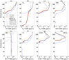 |
Fig. 6 VMR proflies of (а) О, (b) О2, (с) О3, (d) OH, (e) HCl, (f) Cl, (g) COC1, and (h) CICCО3 following the same design as in Figure 3. |
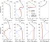 |
Fig. 7 VMR profiles of (a) NO, (b) NО2, (c) NО3, (d) N, (e) HNO, (f) HNО2, (g) HNО3, and (h) N2О following the same design as in Figure 3. |
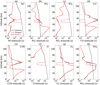 |
Fig. 8 Chemical (solid) and transport (dashed) timescales of (a) SO, (b) S02, (c) S03, (d) CO, (e) COS, (f) O, (g) O2, and (h) NO2 in both the nominal model (black) and Model A (red). We note that the chemical timescale is measured by ni/Li. The transport timescale is measured by teddy = H2IKzz, where H = kBTlmg is the density scale height, kB is the Boltzmann constant, T is the temperature, m is the atmospheric molecular mass, and g is the gravity. |
4.2 Influences of dissolution and the release process on the sulfur system
The SO2 is the primary reservoir of sulfur in Venusian atmospheres and plays a crucial role in the production of SO3, H2SO4, and subsequent cloud formation. It is likely to have originated from volcanic outgassing at the surface (Esposito et al. 1988). Based on series remote sensing and in situ observations by Venus Express, Venera, and VEGA, a dramatic variation of SO2 in and above the clouds attests that its VMR drops from 150 ppmv at 40 km to ~0.1 ppmv at 70 km (Vandaele et al. 2017). As there are only ~30 ppmv H2O in the lower atmosphere, it is insufficient to consume all the depleted SO2 by cloud formation. The formation of such a substantial depletion is still a subject of debate (Petkowski et al. 2024).
In this study, we adopted the dissolution of SO2 from Rimmer et al. (2021) in our nominal model to match the observations of SO2 above 60 km (e.g. Belyaev et al. 2012, 2014; Encrenaz et al. 2013). Figure 9 shows the crucial sources and sinks of SO2 in the nominal model. The photolysis of SO2 regulates its abundances above 100 km, where it is in equilibrium with the recombination of SO and O. SO2 is quickly consumed by (net) dissolution at 58–70 km, which is compensated by the release of SO2 caused by droplet evaporation at 40–58 km. We indicate that such a rapid dissolution-release cycle facilitates a large upward SO2 flux at 58 km and, consequently, a sharp gradient of its VMR. The eddy flux of SO2 at 58 km in the nominal model reaches 2.7× 1012 cm−2 s−1, which is larger than that of Bierson & Zhang (2020) by a factor of four. SO2 is regulated by a diffusion process in the lower atmosphere (Fig. 8), although there is a significant chemical source of SO2 near 40 km caused by the reaction between COS and SO3.
It is worth noting that the rate coefficient of SO2 dissolution is experientially determined by Rimmer et al. (2021) using Henry’s law, and its confirmation through experiments is pending, although the nominal model shows the closest agreement with the observations. Since the liquid SO2 does not interact with other species in the model’s chemical network, its role is simply to serve as a substitute medium to adjust the amount of SO2 in order to match the observed data. Future experimental verification is crucial for gaining deeper insights into the process of SO2 consumption.
Notably, a significant increase in SO abundance appears at 70 km (Fig. 3). The value of this peak is about an order of magnitude larger than the simulations of previous studies such as Zhang et al. (2012), which has a significant effect on the O2 abundance (discussed later). To figure out the formation of this increase, the primary source and sink reactions of SO are illustrated in Fig. 10. SO is mainly produced by the photolysis of SO2 above 70 km and removed by its recombination with O at 70–105 km and photolysis above 105 km. ClO also contributes to 10% of the SO loss near 80 km:

At 60–70 km, SO seems to be regulated by its rapid conversion with S2O2:

However, these two reactions make minimal contributions to pushing the equilibrium state of SO due to the exceedingly short lifetime of S2O2 (Frandsen et al. 2016). In this scenario, S contributes to half of the SO production at 70 km. Another SO (65–72 km), NO2 (70–75 km) and O2 (50–70 km) are responsible for the removal of SO in this region:

As for S, it is entirely produced by the self-combination of SO and eliminated by O2 at 70 km. Thus, we are able to extract the transforming pathway between the mentioned sulfur species at 70 km:

Interestingly, S and SO2 abundances also show slight increases at this altitude (Figs. 3 and 4). Since both S and SO are regulated by internal recycling, the only external factor of the S element must be from SO2; that is, the regulation by the dissolution and release between liquid SO2 in the clouds.
To examine this hypothesis, we performed a sensitivity test for the dissolution rate of SO2. Both the dissolution and release rate constants (R293–295) were simultaneously scaled from the nominal values to zero, as shown in Fig. 11. According to the results, both the peaks of SO and SO2 are sensitive to the dissolution rate. Their altitudes and values increase as the dissolution is weakened. In this study, the total SO2 is composed of gas SO2 and liquid SO2 stored in the clouds. In the presence of liquid SO2, the system needs to find the equilibrium state among the photolysis, the chemical source, and the gas-liquid exchange for the SO2 at 70 km. Once its abundance is reduced by photolysis, the dissolution rate decreases and the SO2 gas could be rapidly compensated by the release from the clouds. In other words, the liquid SO2 is able to buffer the S element in this chemical system, which is attributed to the increase of SO at 70 km.
 |
Fig. 9 Two left panels show the reaction rates (a) and their contributions (b) to the chemical sink of SO2 in the nominal model. The two right panels show the rates (c) and contributions (d) to the chemical source in the nominal model. Only reactions with a maximum contribution (over altitude) larger than 0.3 are presented. |
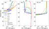 |
Fig. 11 VMR profiles of (a) SO and (b) SO2, and (c) SO2(l) at 70 km in the sensitivity test for SO2 dissolution. The dissolution and release rate constants (R293–295) are simultaneously scaled from the nominal values to zero (black to red). We mark the SO VMR from Zhang et al. (2012, pink triangle) for comparison. Observations are shown in gray. |
4.3 A novel mechanism to eliminate O2 at 70 km
Venus possesses an atmosphere that is highly oxidized. Based on the evaluated high column photolysis rates of CO2 and the rapid combination of O to produce O2 by three-body association and certain catalytic reactions, O2 should have been abundant in the stratosphere of Venus (Krasnopolsky 2006b). However, there has not yet been any direct observation of O2 on Venus. Trauger & Lunine (1983) gave an upper limit of 0.3 ppmv to the O2 VMR above the cloud top based on the resolving power of their triple pressure-scanned Fabry-Perot interferometer. This upper limit was subsequently revised by Krasnopolsky (2006b) as 8×1017 cm−2 to the O2 column abundance above 62 km. Indirect evidence of the presence of O2 was derived by Connes et al. (1979), who detected intense airglow from O2(1Δ) at 1.27 µm on both the light and the dark sides of Venus, using a ground-based, high-resolution Fourier-transform spectrometer. Recently, O atoms have been detected with a column density of 0.7~3.8×1017 cm−2 on Venus (Hübers et al. 2023). This finding further supports the likelihood of the presence of O2.
Nevertheless, in most photochemical models including this study, the simulated column densities of O2 in the middle atmosphere significantly exceed the upper limit. This is a longstanding problem in the Venusian atmospheric chemical modeling. Krasnopolsky & Parshev (1981) and Yung & Demore (1982) introduced a chlorine-catalyzed destruction mechanism that regulates the O2 abundance in the Venusian middle atmosphere. It was then adopted by Mills (1998) and Zhang et al. (2012), using the equilibrium constants of COCl exceeding the measurements (Nicovich et al. 1990; Sander et al. 2003) by two orders of magnitude and a factor of 40, respectively, to improve the fitting of their models. Although the COCl cycle is also included in our model, we used a more moderate equilibrium constant adopted from Bierson & Zhang (2020). In this case, interestingly, the simulated O2 VMR in this study significantly decreases with decreasing altitude at 70 km (Fig. 6) and reaches the same magnitude as Zhang et al. (2012).
To further explore the oxygen chemistry, we illustrate the sink reactions of O2 in Fig. 12. According to the results, the reactions with either SO or S take over the consumption of O2 in a narrow layer slightly below 70 km. This varies from the COCl cycle in many previous studies. As we already mentioned, it could be attributed to the buffering effect of liquid SO2 in the clouds that leads to the increases of the sulfur species in this region. This mechanism contributes to a large column-loss rate of 1.96×1011 cm−2 s−1 in 60–70 km, efficiently suppressing the downward transport of O2. It means that sulfur cycle could have a superior regulation on O2 in this narrow layer and indicates that it may have potential contributions to the long-standing problem of the overestimated O2 abundance:

The consumption of O2 by COCl is less efficient than the mentioned processes in our model. However, this does not mean that the COCl cycle does not work on O2 consumption. Instead, it indirectly affects the O2 abundance by eliminating O above 80 km, where O2 is mainly produced by the self-combination of O atoms:

5 Conclusions
This study was carried out to investigate the atmospheric chemistry on Venus, with a particular focus on the influence of the SO2 dissolution in the clouds. We developed an open-access photochemistry-transport model for the Venusian atmosphere that extends from the surface up to 112 km with a vertical resolution of 2 km. This model incorporates current knowledge of the Venusian atmospheric chemistry into the VULCAN framework, the vertical eddy diffusion recently retrieved by the Venus Express observations, and the radiative transfer containing the absorption and scattering of the gases, the Mie scattering of the cloud droplets, and the absorption of the UV absorber. The model involves the dissolution of SO2 in the clouds and the adjusted COS chemistry based on the detected COS abundance. A comprehensive examination of the abundances of the crucial species, along with the primary chemistry of sulfur and oxygen species, is presented in this paper.
The simulated abundance profiles of SO, SO2, CO, COS, O, O2, O3, HCl, and NO basically agree with the observations, and some differences are discussed in the context. The increase of cloud Kzz does not have a significant direct effect on the chemistry in the middle and lower atmospheres of Venus although it might play a role in the cloud formation. This could be attributed to either the extremely low abundances or the high transport timescales of the species in the cloud layer.
The net dissolution of SO2 is effective at 58–70 km. It is compensated by the release of SO2 at 40–58 km which is attributed to the droplet evaporation. It is the rapid dissolution-release cycle that facilitates the large upward SO2 flux and the formation of the distinct gradient of its abundance beginning at 55 km.
The SO abundance sees a significant increase at 70 km which is larger than the predictions of previous studies by an order of magnitude. S and SO2 also show slight increases at the same altitude. These structures are sensitive to the dissolution rate. We propose that they are attributed to the buffering effects of liquid SO2 in the clouds, which compensate the gas through evaporation once its abundance decreases by photolysis. This mechanism takes the sulfur element at this altitude to a novel equilibrium state between gas internal cycles and gas-liquid exchange.
We find a novel mechanism to eliminate O2 at 70 km that is driven by sulfur cycle. O2 decreases significantly at this altitude, reaching the same magnitude as previous studies, although we used a more moderate COCl cycle eliminating O2. It is efficiently eliminated by SO+O, which is regulated by the significant increase of SO in this region as mentioned. Instead, COCl has a less direct consumption of O2, but it indirectly affects it by eliminating O. Thus, we emphasize the superior regulation of the sulfur cycle on O2 in this layer and the potential contributions of it to the long-standing problem of the overestimation of the O2 abundance in the simulations.
In this model, the rate coefficients of a considerable portion of the chemical reactions are empirically obtained and have not been experimentally verified, particularly those involving sulfur species. The supplement of experimental data is essential for the improvement of the atmospheric chemical study of Venus. In addition, the sulfuric acid clouds may exhibit significant interactions with the atmospheric chemistry. It is crucial to incorporate self-consistent cloud formation in future studies.
Acknowledgments
We thank Paul B. Rimmer and Carver J. Bierson for their constructive suggestions on handling the sulfur chemistry. We thank Shang-Min Tsai for the helpful tips to understand the framework. This work is supported by the National Natural Science Foundation of China (Grant 42305135, 42275060). Longkang Dai is also supported by Natural Science Foundation of Hunan Province (Grant 2023JJ40664).
Data availability
The data in this study and the chemical reactions are collected at: https://doi.org/1S.5281/zenodo.12696879. The source code of this model is publicly available at: https://github.com/dai-lk/VULCAN-Venus.
References
- Ando, H., Imamura, T., Tsuda, T., et al. 2015, J. Atmos. Sci., 72, 2318 [NASA ADS] [CrossRef] [Google Scholar]
- Ando, H., Imamura, T., Tellmann, S., et al. 2020, Sci. Rep., 10, 3448 [Google Scholar]
- Arney, G., Meadows, V., Crisp, D., et al. 2014, J. Geophys. Res. (Planets), 119, 1860 [NASA ADS] [CrossRef] [Google Scholar]
- Belyaev, D. A., Montmessin, F., Bertaux, J.-L., et al. 2012, Icarus, 217, 740 [CrossRef] [Google Scholar]
- Belyaev, D., Fedorova, A., Piccialli, A., et al. 2014, in 40th COSPAR Scientific Assembly, 40, B0.7-8-14 [Google Scholar]
- Bertaux, J.-L., Widemann, T., Hauchecorne, A., Moroz, V. I., & Ekonomov, A. P. 1996, J. Geophys. Res., 101, 12709 [NASA ADS] [CrossRef] [Google Scholar]
- Bertaux, J.-L., Vandaele, A.-C., Korablev, O., et al. 2007, Nature, 450, 646 [NASA ADS] [CrossRef] [Google Scholar]
- Bézard, B., & de Bergh, C. 2007, J. Geophys. Res.: Planets, 112, E4 [Google Scholar]
- Bézard, B., de Bergh, C., Crisp, D., & Maillard, J.-P. 1990, Nature, 345, 508 [CrossRef] [Google Scholar]
- Bézard, B., de Bergh, C., Fegley, B., et al. 1993, Geophys. Res. Lett., 20, 1587 [Google Scholar]
- Bierson, C. J., & Zhang, X. 2020, J. Geophys. Res. (Planets), 125, e06159 [NASA ADS] [Google Scholar]
- Bjoraker, G. L., Larson, H. P., Mumma, M. J., Timmermann, R., & Montani, J. L. 1992, in AAS/Division for Planetary Sciences Meeting Abstracts, 24, 30.04 [NASA ADS] [Google Scholar]
- Connes, P. 1967, Publ. Observatoire Haute-Provence, 9, 1230 [NASA ADS] [Google Scholar]
- Connes, P., Noxon, J. F., Traub, W. A., & Carleton, N. P. 1979, ApJ, 233, L29 [NASA ADS] [CrossRef] [Google Scholar]
- Cotton, D. V., Bailey, J., Crisp, D., & Meadows, V. 2012, Icarus, 217, 570 [NASA ADS] [CrossRef] [Google Scholar]
- Crisp, D. 1986, Icarus, 67, 484 [NASA ADS] [CrossRef] [Google Scholar]
- Dai, L., Zhang, X., & Cui, J. 2022a, MNRAS, 515, 817 [NASA ADS] [CrossRef] [Google Scholar]
- Dai, L., Zhang, X., Shao, W. D., Bierson, C. J., & Cui, J. 2022b, J. Geophys. Res. (Planets), 127, e07060 [Google Scholar]
- Dai, L., Shao, W., Gu, H., & Sheng, Z. 2023, A&A, 679, A155 [NASA ADS] [CrossRef] [EDP Sciences] [Google Scholar]
- de Bergh, C., Bezard, B., Owen, T., et al. 1991, Science, 251, 547 [NASA ADS] [CrossRef] [Google Scholar]
- Donahue, T. M. 1999, Icarus, 141, 226 [NASA ADS] [CrossRef] [Google Scholar]
- Encrenaz, T., Greathouse, T. K., Richter, M. J., et al. 2013, A&A, 559, A65 [NASA ADS] [CrossRef] [EDP Sciences] [Google Scholar]
- Encrenaz, T., Moreno, R., Moullet, A., Lellouch, E., & Fouchet, T. 2015, Planet. Space Sci., 113, 275 [Google Scholar]
- Encrenaz, T., Greathouse, T. K., Marcq, E., et al. 2020, A&A, 639, A69 [NASA ADS] [CrossRef] [EDP Sciences] [Google Scholar]
- Esposito, L. W., Knollenberg, R. G., Marov, M. I., Toon, O. B., & Turco, R. P. 1983, in Venus, Tucson, AZ: University of Arizona Press, 484 [Google Scholar]
- Esposito, L. W., Copley, M., Eckert, R., et al. 1988, J. Geophys. Res., 93, 5267 [NASA ADS] [CrossRef] [Google Scholar]
- Fedorova, A., Korablev, O., Vandaele, A. C., et al. 2008, J. Geophys. Res. (Planets), 113, E00B22 [CrossRef] [Google Scholar]
- Fegley, B., Zolotov, M. Y., & Lodders, K. 1997, Icarus, 125, 416 [NASA ADS] [CrossRef] [Google Scholar]
- Frandsen, B. N., Wennberg, P. O., & Kjaergaard, H. G. 2016, Geophys. Res. Lett., 43, 11, 146 [Google Scholar]
- Heays, A. N., Bosman, A. D., & van Dishoeck, E. F. 2017, A&A, 602, A105 [NASA ADS] [CrossRef] [EDP Sciences] [Google Scholar]
- Heng, K., Malik, M., & Kitzmann, D. 2018, ApJS, 237, 29 [CrossRef] [Google Scholar]
- Herrick, R. R., & Hensley, S. 2023, Science, 379, 1205 [NASA ADS] [CrossRef] [Google Scholar]
- Hoffman, J. H., Hodges, R. R., Donahue, T. M., & McElroy, M. M. 1980, J. Geophys. Res., 85, 7882 [NASA ADS] [CrossRef] [Google Scholar]
- Hübers, H.-W., Richter, H., Graf, U. U., et al. 2023, Nat. Commun., 14, 6812 [CrossRef] [Google Scholar]
- Imamura, T., Ando, H., Tellmann, S., et al. 2017, Earth Planets Space, 69, 137 [NASA ADS] [CrossRef] [Google Scholar]
- Iwagami, N., Ohtsuki, S., Tokuda, K., et al. 2008, Planet. Space Sci., 56, 1424 [NASA ADS] [CrossRef] [Google Scholar]
- Jessup, K. L., Marcq, E., Mills, F., et al. 2015, Icarus, 258, 309 [NASA ADS] [CrossRef] [Google Scholar]
- Jiang, C. Z., Rimmer, P. B., Lozano, G. G., et al. 2024, Sci. Adv., 10, eadg8826 [NASA ADS] [CrossRef] [Google Scholar]
- Knollenberg, R. G., & Hunten, D. M. 1980, J. Geophys. Res., 85, 8039 [CrossRef] [Google Scholar]
- Krasnopolsky, V. A. 1985, Planet. Space Sci., 33, 109 [NASA ADS] [CrossRef] [Google Scholar]
- Krasnopolsky, V. A. 2006a, Icarus, 182, 80 [NASA ADS] [CrossRef] [Google Scholar]
- Krasnopolsky, V. A. 2006b, Planet. Space Sci., 54, 1352 [NASA ADS] [CrossRef] [Google Scholar]
- Krasnopolsky, V. A. 2007, Icarus, 191, 25 [NASA ADS] [CrossRef] [Google Scholar]
- Krasnopolsky, V. A. 2010a, Icarus, 208, 539 [NASA ADS] [CrossRef] [Google Scholar]
- Krasnopolsky, V. A. 2010b, Icarus, 209, 314 [NASA ADS] [CrossRef] [Google Scholar]
- Krasnopolsky, V. A. 2012, Icarus, 218, 230 [NASA ADS] [CrossRef] [Google Scholar]
- Krasnopolsky, V. A. 2013, Planet. Space Sci., 85, 78 [Google Scholar]
- Krasnopolsky, V. A. 2014, Icarus, 237, 340 [NASA ADS] [CrossRef] [Google Scholar]
- Krasnopolsky, V. A., & Parshev, V. A. 1980, Cosmic Res., 17, 763 [Google Scholar]
- Krasnopolsky, V. A., & Parshev, V. A. 1981, Nature, 292, 610 [CrossRef] [Google Scholar]
- Krasnopolsky, V. A., & Pollack, J. B. 1994, Icarus, 109, 58 [NASA ADS] [CrossRef] [Google Scholar]
- Lane, W. A., & Opstbaum, R. 1983, Icarus, 54, 48 [NASA ADS] [CrossRef] [Google Scholar]
- Lefèvre, M., Marcq, E., & Lefèvre, F. 2022, Icarus, 386, 115148 [CrossRef] [Google Scholar]
- Mahieux, A., Vandaele, A. C., Robert, S., et al. 2015a, Planet. Space Sci., 113, 193 [NASA ADS] [CrossRef] [Google Scholar]
- Mahieux, A., Wilquet, V., Vandaele, A. C., et al. 2015b, Planet. Space Sci., 113, 264 [Google Scholar]
- Mahieux, A., Robert, S., Mills, F. P., et al. 2023a, Icarus, 399, 115556 [NASA ADS] [CrossRef] [Google Scholar]
- Mahieux, A., Robert, S., Piccialli, A., Trompet, L., & Vandaele, A. C. 2023b, Icarus, 405, 115713 [NASA ADS] [CrossRef] [Google Scholar]
- Malik, M., Kitzmann, D., Mendonça, J. M., et al. 2019, AJ, 157, 170 [Google Scholar]
- Marcq, E., Encrenaz, T., Bézard, B., & Birlan, M. 2006, Planet. Space Sci., 54, 1360 [NASA ADS] [CrossRef] [Google Scholar]
- Marcq, E., Bézard, B., Drossart, P., et al. 2008, J. Geophys. Res. (Planets), 113, E00B07 [CrossRef] [Google Scholar]
- Marcq, E., Lellouch, E., Encrenaz, T., et al. 2015, Planet. Space Sci., 113, 256 [Google Scholar]
- Marcq, E., Mills, F. P., Parkinson, C. D., & Vandaele, A. C. 2018, Space Sci. Rev., 214, 10 [NASA ADS] [CrossRef] [Google Scholar]
- Marcq, E., Baggio, L., Lefèvre, F., et al. 2019, Icarus, 319, 491 [NASA ADS] [CrossRef] [Google Scholar]
- Marcq, E., Bézard, B., Reess, J. M., et al. 2023, Icarus, 405, 115714 [NASA ADS] [CrossRef] [Google Scholar]
- Mills, F. P. 1998, Ph.D. Thesis, California Institute of Technology, USA [Google Scholar]
- Montmessin, F., Bertaux, J. L., Lefèvre, F., et al. 2011, Icarus, 216, 82 [NASA ADS] [CrossRef] [Google Scholar]
- Nicovich, J. M., Kreutter, K. D., & Wine, P. H. 1990, J. Chem. Phys., 92, 3539 [NASA ADS] [CrossRef] [Google Scholar]
- Oyama, V. I., Carle, G. C., Woeller, F., & Pollack, J. B. 1979, Science, 203, 802 [NASA ADS] [CrossRef] [Google Scholar]
- Oyama, V. I., Carle, G. C., Woeller, F., et al. 1980, J. Geophys. Res., 85, 7891 [NASA ADS] [CrossRef] [Google Scholar]
- Parkinson, C. D., Gao, P., Esposito, L., et al. 2015, Planet. Space Sci., 113, 226 [Google Scholar]
- Petkowski, J. J., Seager, S., Grinspoon, D. H., et al. 2024, Astrobiology, 24, 343 [NASA ADS] [CrossRef] [Google Scholar]
- Pollack, J. B., Dalton, J. B., Grinspoon, D., et al. 1993, Icarus, 103, 1 [NASA ADS] [CrossRef] [Google Scholar]
- Rimmer, P. B., Jordan, S., Constantinou, T., et al. 2021, Planet. Sci. J., 2, 133 [NASA ADS] [CrossRef] [Google Scholar]
- Sander, S. P., Friedl, R. R., Golden, D. M., et al. 2003, Chemical kinetics and photochemical data for use in atmospheric studies, evaluation number 14. Tech. rep. (JPL Publication), 02 [Google Scholar]
- Sandor, B. J., & Clancy, R. T. 2012, Icarus, 220, 618 [NASA ADS] [CrossRef] [Google Scholar]
- Sandor, B. J., & Clancy, R. T. 2017, Icarus, 290, 156 [NASA ADS] [CrossRef] [Google Scholar]
- Sandor, B. J., Todd Clancy, R., Moriarty-Schieven, G., & Mills, F. P. 2010, Icarus, 208, 49 [NASA ADS] [CrossRef] [Google Scholar]
- Sato, T. M., & Sagawa, H. 2023, Icarus, 390, 115307 [NASA ADS] [CrossRef] [Google Scholar]
- Schulze-Makuch, D., Grinspoon, D. H., Abbas, O., Irwin, L. N., & Bullock, M. A. 2004, Astrobiology, 4, 11 [CrossRef] [Google Scholar]
- Seiff, A., Schofield, J. T., Kliore, A. J., et al. 1985, Adv. Space Res., 5, 3 [Google Scholar]
- Shao, W. D., Zhang, X., Bierson, C. J., & Encrenaz, T. 2020, J. Geophys. Res. (Planets), 125, e06195 [Google Scholar]
- Stolzenbach, A., Lefèvre, F., Lebonnois, S., & Määttänen, A. 2023, Icarus, 395, 115447 [NASA ADS] [CrossRef] [Google Scholar]
- Sumlin, B. J., Heinson, W. R., & Chakrabarty, R. K. 2018, JQSRT, 205, 127 [NASA ADS] [CrossRef] [Google Scholar]
- Titov, D. V., Ignatiev, N. I., McGouldrick, K., Wilquet, V., & Wilson, C. F. 2018, Space Sci. Rev., 214, 126 [NASA ADS] [CrossRef] [Google Scholar]
- Tomasko, M. G., Smith, P. H., Suomi, V. E., et al. 1980, J. Geophys. Res., 85, 8187 [NASA ADS] [CrossRef] [Google Scholar]
- Trauger, J. T., & Lunine, J. I. 1983, Icarus, 55, 272 [NASA ADS] [CrossRef] [Google Scholar]
- Tsai, S.-M., Lyons, J. R., Grosheintz, L., et al. 2017, ApJS, 228, 20 [NASA ADS] [CrossRef] [Google Scholar]
- Tsai, S.-M., Malik, M., Kitzmann, D., et al. 2021, ApJ, 923, 264 [NASA ADS] [CrossRef] [Google Scholar]
- Tsai, S.-M., Lee, E. K. H., Powell, D., et al. 2023, Nature, 617, 483 [CrossRef] [Google Scholar]
- Tsang, C., Taylor, F., Wilson, C., et al. 2009, Icarus, 201, 432 [NASA ADS] [CrossRef] [Google Scholar]
- Vandaele, A. C., De Mazière, M., Drummond, R., et al. 2008, J. Geophys. Res. (Planets), 113, E00B23 [CrossRef] [Google Scholar]
- Vandaele, A. C., Korablev, O., Belyaev, D., et al. 2017, Icarus, 295, 16 [NASA ADS] [CrossRef] [Google Scholar]
- von Zahn, U., Kumar, S., Niemann, H., & Prinn, R. 1983, in Venus, eds. D. M. Hunten, et al. (Tucson, AZ: University of Arizona Press), 299 [Google Scholar]
- Wilquet, V., Fedorova, A., Montmessin, F., et al. 2009, J. Geophys. Res. (Planets), 114, E00B42 [CrossRef] [Google Scholar]
- Woo, R., & Ishimaru, A. 1981, Nature, 289, 383 [NASA ADS] [CrossRef] [Google Scholar]
- Woo, R., Armstrong, J. W., & Kliore, A. J. 1982, Icarus, 52, 335 [NASA ADS] [CrossRef] [Google Scholar]
- Young, L. 1972, Icarus, 17, 632 [NASA ADS] [CrossRef] [Google Scholar]
- Yung, Y. L., & Demore, W. B. 1982, Icarus, 51, 199 [NASA ADS] [CrossRef] [Google Scholar]
- Yung, Y. L., Liang, M. C., Jiang, X., et al. 2009, J. Geophys. Res. (Planets), 114, E00B34 [CrossRef] [Google Scholar]
- Zhang, X., Liang, M. C., Mills, F. P., Belyaev, D. A., & Yung, Y. L. 2012, Icarus, 217, 714 [NASA ADS] [CrossRef] [Google Scholar]
All Tables
All Figures
|
Fig. 1 (a) Pressure, (b) temperature, and (c) eddy diffusion coefficient profiles adopted in this study. The pressure and temperature profiles are adopted from Seiff et al. (1985). The nominal Kzz profile is adopted from Bierson & Zhang (2020). The red line in panel (c) is the global-mean Kzz profile adopted from Dai et al. (2023), which is tested in our Model A. |
| In the text | |
|
Fig. 2 H2SO4 (red) and H2O (blue) profiles adopted from Bierson & Zhang (2020), and liquid H2SO4 (green) profile adopted from Rimmer et al. (2021). Observations are presented for comparison. |
| In the text | |
|
Fig. 3 VMR profiles of (a) SO, (b) SO2, (c) SO3, and (d) S2O2 in our cases. We note that the nominal results overlap with Model A at most altitudes. The observations (gray), the results from Bierson & Zhang (2020, orange), Rimmer et al. (2021, blue) and Zhang et al. (2012, pink) are also presented for benchmarking purposes. |
| In the text | |
|
Fig. 4 VMR profiles of some other sulfur species in the nominal model. |
| In the text | |
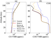 |
Fig. 5 VMR profiles of (a) CO and (b) COS following design as in Figure 3. |
| In the text | |
|
Fig. 6 VMR proflies of (а) О, (b) О2, (с) О3, (d) OH, (e) HCl, (f) Cl, (g) COC1, and (h) CICCО3 following the same design as in Figure 3. |
| In the text | |
|
Fig. 7 VMR profiles of (a) NO, (b) NО2, (c) NО3, (d) N, (e) HNO, (f) HNО2, (g) HNО3, and (h) N2О following the same design as in Figure 3. |
| In the text | |
|
Fig. 8 Chemical (solid) and transport (dashed) timescales of (a) SO, (b) S02, (c) S03, (d) CO, (e) COS, (f) O, (g) O2, and (h) NO2 in both the nominal model (black) and Model A (red). We note that the chemical timescale is measured by ni/Li. The transport timescale is measured by teddy = H2IKzz, where H = kBTlmg is the density scale height, kB is the Boltzmann constant, T is the temperature, m is the atmospheric molecular mass, and g is the gravity. |
| In the text | |
|
Fig. 9 Two left panels show the reaction rates (a) and their contributions (b) to the chemical sink of SO2 in the nominal model. The two right panels show the rates (c) and contributions (d) to the chemical source in the nominal model. Only reactions with a maximum contribution (over altitude) larger than 0.3 are presented. |
| In the text | |
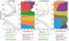 |
Fig. 10 Source and sink reactions of SO following the same design as in Figure 9. |
| In the text | |
|
Fig. 11 VMR profiles of (a) SO and (b) SO2, and (c) SO2(l) at 70 km in the sensitivity test for SO2 dissolution. The dissolution and release rate constants (R293–295) are simultaneously scaled from the nominal values to zero (black to red). We mark the SO VMR from Zhang et al. (2012, pink triangle) for comparison. Observations are shown in gray. |
| In the text | |
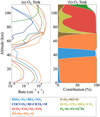 |
Fig. 12 Sink reactions of O2 following the same design as in Figure 9. |
| In the text | |
Current usage metrics show cumulative count of Article Views (full-text article views including HTML views, PDF and ePub downloads, according to the available data) and Abstracts Views on Vision4Press platform.
Data correspond to usage on the plateform after 2015. The current usage metrics is available 48-96 hours after online publication and is updated daily on week days.
Initial download of the metrics may take a while.