| Issue |
A&A
Volume 645, January 2021
|
|
|---|---|---|
| Article Number | L4 | |
| Number of page(s) | 6 | |
| Section | Letters to the Editor | |
| DOI | https://doi.org/10.1051/0004-6361/202039932 | |
| Published online | 24 December 2020 | |
Letter to the Editor
Phosphine in Venus’ atmosphere: Detection attempts and upper limits above the cloud top assessed from the SOIR/VEx spectra
1
Planetary Aeronomy, Royal Belgian Institute for Space Aeronomy, Brussels, Belgium
e-mail: This email address is being protected from spambots. You need JavaScript enabled to view it.
2
Institute of Condensed Matter and Nanosciences, Université catholique de Louvain, Chemin du Cyclotron 2, 1348 Louvain-la-Neuve, Belgium
3
The University of Texas at Austin, Austin, TX, USA
4
Université Paris-Saclay, CNRS, GEOPS, 91405 Orsay, France
Received:
17
November
2020
Accepted:
10
December
2020
Abstract
Context. Recent detection of phosphine (PH3) was reported from James Clerk Maxwell Telescope and Atacama Large Millimetre/submillimetre Array observations. The presence of PH3 on Venus cannot be easily explained in the Venus atmosphere and a biogenic source located at or within the clouds was proposed.
Aims. We aim to verify if the infrared spectral signature of PH3 is present in the spectra of Solar Occultation at Infrared (SOIR). If it is not present, we then seek to derive the upper limits of PH3 from SOIR spectra.
Methods. We analyzed the SOIR spectra containing absorption lines of PH3. We searched for the presence of PH3 lines. If we did not find any conclusive PH3 spectral signatures, we computed the upper limits of PH3.
Results. We report no detection of PH3. Upper limits could be determined for all of the observations, providing strong constraints on the vertical profile of PH3 above the clouds.
Conclusions. The SOIR PH3 upper limits are almost two orders of magnitude below the announced detection of 20 ppb and provide the lowest known upper limits for PH3 in the atmosphere of Venus.
Key words: planets and satellites: atmospheres / infrared: planetary systems / techniques: spectroscopic / methods: data analysis
© L. Trompet et al. 2020
 Open Access article, published by EDP Sciences, under the terms of the Creative Commons Attribution License (https://creativecommons.org/licenses/by/4.0), which permits unrestricted use, distribution, and reproduction in any medium, provided the original work is properly cited.
1. Introduction
In light of the recent publication of Greaves et al. (2020a) reporting on the detection of phosphine above the Venusian clouds, we decided to explore the Solar Occultation at Infrared (SOIR) database in search of a spectral signature of PH3 in the infrared (IR) range. Greaves et al. (2020a) identified a phosphine line in spectra taken by two different instruments, James Clerk Maxwell Telescope (JCMT) and Atacama Large Millimetre/submillimetre Array (ALMA) in June 2017 and March 2019, respectively. They claim that it corresponds to 20 ppb of phosphine at an altitude of 53 to 61 km. In addition to the difficulties in understanding how phosphine can be present in Venus’ atmosphere, this possible detection still needs confirmation and validation from other spectral lines of phosphine.
In this framework, Encrenaz et al. (2020) used a mid-IR (950 cm−1) spectrum from the Texas Echelon CrossEchelle Spectrograph (TEXES) instrument acquired on March 28, 2015. They could not detect any spectral signatures of phosphine and derived an upper limit of 5 ppb. Snellen et al. (2020) reprocessed the ALMA spectra and show that the apparent presence of a phosphine line might actually be a spurious feature from the calibration of the spectra. More recently, Villanueva et al. (2020) have concluded that the line in the JCMT spectra might be due to a SO2 line and that the calibration of ALMA spectra used in Greaves et al. (2020a) might not have been correctly performed. Using updated and corrected ALMA data, Greaves et al. (2020b) revised their conclusion, confirming the detection of PH3 but reducing the observed abundance to a 1 ppb global disk average.
The SOIR instrument has already proven to be very sensitive to the detection and quantification of trace gases (Wilquet et al. 2012; Vandaele et al. 2015; Mahieux et al. 2015a,b) thanks to its solar occultation measurements delivering spectra with a high signal-to-noise ratio (S/N). Providing that the species have a spectral signature in the SOIR instrument’s spectral range, the SOIR dataset can corroborate the possible presence of trace gases in the atmosphere of Venus or, otherwise, help to constrain their upper limits.
2. SOIR description
The SOIR instrument (Nevejans et al. 2006) onboard the ESA Venus Express (VEx) spacecraft (Titov et al. 2006), which is an IR spectrometer sensitive from 2.2 to 4.3 μm, probed the atmosphere of Venus from June 2006 until December 2014. During this time, it performed more than 750 solar occultations of Venus’ middle and upper atmosphere (∼60 to ∼180 km).
SOIR spectra have a resolution varying from 0.11 to 0.21 cm−1 (resolving power of 21500) with increasing wavenumber, the highest onboard VEx. SOIR combined an echelle grating to disperse the light in diffraction orders and an acousto-optical tunable filter (AOTF) as a diffraction order-sorting device. The echelle grating and the AOTF led to a division of the spectral range (2256 to 4369 cm−1) into 94 wavenumber domains corresponding to the diffraction orders, which are simply referred to as “orders” in the following. SOIR delivered height sets of spectra per solar occultation, each of them is referred to as “dataset” hereafter (see Appendix B for more details).
We selected SOIR orders 105 to 110 (see Table 1 for the spectral range of each order) by considering the spectral signature of PH3 in the SOIR spectral range. In this region, CO2 and SO2 also have a spectral signature and Fig. 1 shows the intensities of their theoretical lines.
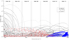 |
Fig. 1. Position of the CO2 (gray), PH3 (red), and SO2 (blue) ro-vibrational transitions in the 2348 to 2501 cm−1 region, corresponding to the SOIR 105 to 111 diffraction orders from HITRAN (Gordon et al. 2017). The line intensities were multiplied by typical Venus abundances, see legend. The SOIR orders are given at the top, with the vertical dashed lines showing their wavenumber extensions. |
SOIR diffraction order to wavenumber range.
3. Methods
The following two different methods were applied to try to detect phosphine in SOIR spectra: a radiative transfer algorithm dedicated to SOIR spectra retrievals named ASIMAT and a new machine learning algorithm. A third method computed the PH3 detection limits for SOIR spectra.
ASIMAT is a Bayesian inversion algorithm using the approach developed by Rodgers (2000). It is set in an onion peeling frame, assuming a spherical symmetry of the atmosphere and fitting the logarithm of the number density of the targeted species. It accounts for the slit projected size at the impact point and for absorption line saturation (Mahieux et al. 2015a,c). ASIMAT successfully retrieved CO2, CO, HCl, HF, H2O, and SO2 from the SOIR spectra. For this study, we implemented a specific scheme to distinguish between a real detection and an upper limit value. The approach is similar to what was done in Korablev et al. (2019) for the Martian methane detection with the NOMAD-SO/ExoMars instrument. The posterior error covariance matrix was computed as the sum of the covariance matrices of the smoothing error and the retrieval noise error (see Eq. (3.31) from Rodgers 2000). The square root of the diagonal of this matrix returned the retrieval detection limit at each altitude for a given species. We assimilated a retrieved number density lower than 3.2 times this value as a non-detection. We computed two inversions for each spectral set: the first one by considering CO2 and PH3 (and SO2 for order 110), and the second one by considering only CO2. We compared the root mean square (rms) for each spectrum fit, and only kept the ones that have a lower rms when retrieving CO2 + PH3 + SO2 than when only retrieving CO2 + SO2.
An alternative attempt to detect PH3 was carried out with a machine learning tool that had already been used to detect the CO2 quadrupole and to infer the absence of methane in NOMAD-SO spectra (Schmidt et al. 2020). The method aims to summarize the dataset with statistical endmembers, hereafter “sources”. First, data are pretreated to remove the baseline and converted into absorbance. The method consists of a linear blind source separation under positivity constraints and uses the probabilistic sparse Non-negative Matrix Factorization (psNMF) described in Hinrich & Mørup (2018). Appendix E provides more information on this analysis.
In addition to these detection methods, we determined the detection limits (DLs) of PH3 in SOIR spectra in the volume mixing ratio (VMR). For each SOIR spectrum, we compared the measurement noise to a synthetic spectrum of PH3 simulated by considering the SOIR instrumental function. We considered that a clear detection of a PH3 line in SOIR spectra should be at least 3.2 times higher than the measurement noise. Appendix F contains a description of this method.
4. Results
Neither the radiative transfer algorithm nor the machine learning algorithm could infer any real detection of PH3 lines for any of the orders selected. In orange, Fig. 2 shows an example of the residual of the SOIR spectrum at 74 km subtracted by the ASIMAT CO2 fit for order 108. We see that several lines of the synthetic PH3 spectrum (blue) are already much stronger than the residual. We see no clear presence of PH3 lines in the SOIR spectrum.
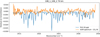 |
Fig. 2. Example of spectrum for orbit 108.1 order 108 bin 2 at a tangent altitude of 74 km. The SOIR spectrum subtracted by the ASIMAT CO2 fit is plotted in orange. The synthetic spectrum of 20 ppb of PH3 is plotted in blue. |
Figure 3 shows an example from the machine learning algorithm for order 106 where one of the sources is clearly identified as CO2 (above panel), but no source could be identified as PH3. In the lower panel, the blue curve corresponds to a source with the highest contribution APH3 to a synthetic PH3 spectrum (black curve).
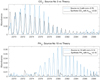 |
Fig. 3. Example of source derived from the machine learning algorithm (in blue) compared to synthetic spectrum (in black) for order 106. The synthetic spectrum is rescaled with fitted linear contribution of CO2 (ACO2) and PH3 (APH3). The correlation coefficient between source and synthetic spectra is noted corr. Above, the source is identified as CO2 (significant ACO2 > 0.5 and high corr > 0.3). Below the closest source (highest APH3) to the PH3 synthetic spectrum is not coherent with its presence (APH3 < 0.5 and corr < 0.3). |
The DLs were computed for two cases. The first case is a constant PH3 VMR up to 190 km. The second case is a constant PH3 VMR up to 68 km. The choice of this last case comes from the top panel of Fig. 9 from Greaves et al. (2020a) where 68 km corresponds to the highest altitude where the PH3 VMR is higher than 0.1 ppb.
Figure 4 shows the DL profiles for orders 105 to 110 for the first case. They have the typical shape expected for solar occultation measurements: from higher altitudes, they decrease with lower tangent altitudes until they increase again because of the progressive presence of clouds and hazes, which decreases the S/N along the whole spectra. The tangent altitude of lowest detection limit (ALDL) varies from one occultation to another depending on the latitude covered, the atmosphere variability, the cloud-deck height, and the strength of the PH3 lines in the spectral order sounded.
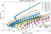 |
Fig. 4. Detection limits as a function of altitude. Colors are the different diffraction orders of SOIR. The blue vertical line corresponds to 20 ppb. The spectral range of the diffraction orders are provided in Table 1. |
The DLs for orders 109 and 110 are above 20 ppb, but those for orders 105 to 108 are well below 20 ppb. We expect some strong variations in the DLs with respect to the diffraction orders. The PH3 line intensities are stronger in orders 105 and 106 and decrease in orders 107 to 110. Figure 4 clearly shows this variation in PH3 lines intensities.
The altitude of interest is closer to 60 km and thus a few kilometers below the typical ALDL. For order 108, the lowest DL is 3 ppb at 67 km and 4 ppb at 61 km (the lowest tangent altitude probed). For order 107, the lowest DL is 0.7 ppb at 67 km and 2 ppb at 61 km. For order 106, the lowest DL is 0.3 ppb at 69 km and 1 ppb at 65 km. For order 105, the lowest DL is 0.2 ppb at 69 km and 0.4 ppb at 61 km.
The DLs lower than 20 ppb and below 62 km corresponds to ten different datasets of SOIR and five different occultations. The DLs below 20 ppb and below 61 km correspond to six datasets from four different occultations.
The SOIR datasets presented here mostly cover latitudes above 60° north. Still eleven datasets cover the latitudes below 60°, corresponding to three different occultations. As seen in Fig. 5, they correspond to latitudes 6.67° (orbit 108.1, orders 105 to 108), −30.96° (orbit 446.1, order 108), and −9.11° (orbit 591.1, order 105). For the dataset corresponding to orbit 446.1 order 108 bin 2, the ALDL is at 62 km with a detection limit of 8 ppb and at 61 km, and the DL is still 9 ppb. For orbit 108.1 order 107 bin 2, the DL at 62 km is 7 ppb.
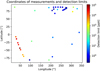 |
Fig. 5. Latitude and longitude coverage of ALDL for SOIR datasets. |
ASIMAT also derives DLs and the results are the same as the ones shown in this section. The machine learning algorithm DL is estimated from those derived in Schmidt et al. (2020) for CH4 lines at 3067.3 cm−1, which are lost in dominant H2O lines in a realistic synthetic dataset, including nonlinear radiative transfer and an instrumental effect. In this case, the detection limit was with a noise variance of 0.001 between 500 ppt (mean absorption bands = 0.0092, S/N = 0.9) and 100 ppt (mean absorption bands = 0.00018, S/N = 0.1). Assuming the same behavior, we estimate that the machine learning algorithm PH3 DL for SOIR spectra is thus 0.5 ppb. This value is similar to the lowest DL in Table 2.
SOIR detection limits below 20 ppb for a constant VMR of phosphine below 180 km (DL1) and 68 km (DL2) and no phosphine above the respective altitude.
For the second case (no PH3 above 68 km), there are two orbits with DLs below 20 ppb: orbit 108.1 and 1250.1. Table 2 summarizes the DLs for a VMR of phosphine until 68 km (column DL2). For comparison, the corresponding DLs of the first case are also provided in column DL1.
5. Discussion and conclusions
We did not detect any phosphine in the SOIR spectra using the two completely different and independent detection methods described above. By considering a constant phosphine VMR, we derived SOIR DLs as low as 0.2 ppb at 69 km with still multiple DLs lower than 20 ppb from 60 to 95 km (see Fig. 4). For a more stringent case of no phosphine above 68 km, a constant volume mixing ratio below 68 km, and by considering only the latitudes between −60° and 60°, the lowest DL is 2 ppb at 65 km.
There is a difference in the time of measurements as SOIR datasets with DLs lower than 20 ppb extend from August 2006 until January 2010 and the spectra used by Greaves et al. (2020a) were recorded in June 2017 and March 2019. Another difference is that SOIR scanned a localized region of the Venus terminator, while the spectra from Greaves et al. (2020a) cover more than 15° of latitude in the Venus disk, as seen from the Earth. These differences might be important if phosphine is really present in Venus’ atmosphere and if the process producing phosphine is localized and varies in time.
Acknowledgments
Venus Express is a planetary mission from the European Space Agency (ESA). We wish to thank all ESA members who participated in the mission, in particular, H. Svedhem and D. Titov. The research program was supported by the Belgian Federal Science Policy Office and the European Space Agency (ESA, PRODEX program, contracts C 90268, 90113, 17645, 90323, and 4000107727). A. Mahieux was supported by the Marie Sklodowska-Curie Action from the European Commission under grant number 838587. This work was supported by the Belgian Fonds de la Recherche Scientifique – FNRS under grant number 30442502 (ET-HOME). SR thanks BELSPO for the FED-tWIN funding (Prf-2019-077 - RT-MOLEXO). F. Schmidt acknowledges support from the “Institut National des Sciences de l’Univers” (INSU), the “Centre National de la Recherche Scientifique” (CNRS) and “Centre National d’Etudes Spatiales” (CNES) through the “Programme National de Planétologie”. We wish to thank the referee for his valuable comments and suggestions that improved the readability of this Letter.
References
- Butler, R. A., Sagui, L., Kleiner, I., & Brown, L. R. 2006, J. Mol. Spectr., 238, 178 [CrossRef] [Google Scholar]
- Chamberlain, S., Mahieux, A., Robert, S., et al. 2020, Icarus, 346, 113819 [CrossRef] [Google Scholar]
- Encrenaz, T., Greathouse, T., Marcq, E., et al. 2020, A&A, 643, L5 [NASA ADS] [CrossRef] [EDP Sciences] [Google Scholar]
- Gordon, I. E., Rothman, L. S., Hill, C., et al. 2017, J. Quant. Spectr. Rad. Transf., 203, 3 [Google Scholar]
- Greaves, J. S., Richards, A. M., Bains, W., et al. 2020a, Nat. Astron., in press [arXiv:2009.06593] [Google Scholar]
- Greaves, J. S., Richards, A. M. S., Bains, W., et al. 2020b, ArXiv e-prints [arXiv:2011.08176] [Google Scholar]
- Hinrich, J. L., & Mørup, M. 2018, in Probabilistic Sparse Non-negative Matrix Factorization (Springer Verlag), Lect. Notes Comput. Sci., 10891, 488 [Google Scholar]
- IUPAC 2008, IUPAC Compendium of Chemical Terminology (IUPAC) [Google Scholar]
- Keating, G. M., Bertaux, J. L., Bougher, S. W., et al. 1985, Adv. Space Res., 5, 117 [NASA ADS] [CrossRef] [Google Scholar]
- Korablev, O., Vandaele, A. C. A. A. C., Montmessin, F., et al. 2019, Nature, 568, 517 [CrossRef] [Google Scholar]
- Mahieux, A., Vandaele, A., Bougher, S., et al. 2015a, Planet. Space Sci., 113, 309 [NASA ADS] [CrossRef] [Google Scholar]
- Mahieux, A., Wilquet, V., Vandaele, A. C., et al. 2015b, Planet. Space Sci., 113, 264 [CrossRef] [Google Scholar]
- Mahieux, A., Vandaele, A. C., Robert, S., et al. 2015c, Planet. Space Sci., 113, 347 [NASA ADS] [CrossRef] [Google Scholar]
- Mahieux, A., Vandaele, A. C., Robert, S., et al. 2015d, Planet. Space Sci., 113, 193 [CrossRef] [Google Scholar]
- Nevejans, D., Neefs, E., Van Ransbeeck, E., et al. 2006, Appl. Opt., 45, 5191 [CrossRef] [Google Scholar]
- Nikitin, A. V., Ivanova, Y. A., Rey, M., et al. 2017, J. Quant. Spectr. Rad. Transf., 203, 472 [CrossRef] [Google Scholar]
- Rodgers, C. D. 2000, in Inverse Methods for Atmospheric Sounding (World Scientific), Ser. Atmos. Ocean. Planet. Phys., 2, 238 [Google Scholar]
- Schmidt, F., Mermy, G. C., Erwin, J., et al. 2020, J. Quant. Spectr. Rad. Transf., 259, 107361 [CrossRef] [Google Scholar]
- Snellen, I. A. G., Guzman-Ramirez, L., Hogerheijde, M. R., Hygate, A. P. S., & van der Tak, F. F. S. 2020, A&A, 644, L2 [NASA ADS] [CrossRef] [EDP Sciences] [Google Scholar]
- Tarrago, G., Lacome, N., Lévy, A., et al. 1992, J. Mol. Spectr., 154, 30 [CrossRef] [Google Scholar]
- Titov, D. V., Svedhem, H., McCoy, D., et al. 2006, Cosm. Res., 44, 334 [NASA ADS] [CrossRef] [Google Scholar]
- Trompet, L., Mahieux, A., Ristic, B., et al. 2016, Appl. Opt., 55, 9275 [CrossRef] [Google Scholar]
- Vandaele, A. C., Mahieux, A., Robert, S., et al. 2013, Opt. Exp., 21, 21148 [CrossRef] [Google Scholar]
- Vandaele, A. C., Neefs, E., Drummond, R., et al. 2015, Planet. Space Sci., 119, 233 [CrossRef] [Google Scholar]
- Villanueva, G., Cordiner, M., Irwin, P., et al. 2020, Nat. Astron., submitted [arXiv:2010.14305] [Google Scholar]
- Wilquet, V., Drummond, R., Mahieux, A., et al. 2012, Icarus, 217, 875 [NASA ADS] [CrossRef] [Google Scholar]
- Zasova, L. V., Ignatiev, N., Khatuntsev, I., & Linkin, V. 2007, Planet. Space Sci., 55, 1712 [NASA ADS] [CrossRef] [Google Scholar]
Appendix A: The SOIR instrument
The SOIR detector counted 320 columns of pixels along its wavenumber axis and 24 illuminated rows (among 256 in total) along its spatial axis. The spectral width of a pixel varied from 0.06 to 0.12 cm−1 with increasing order. The instrument slit was aligned to the Venus limb, such that the detector’s spatial axis was parallel to the limb. Because of telemetry limitations, all of the illuminated rows along the spatial axis were not transmitted to Earth, but they were summed up on board in two spatial bins, thus taken at two slightly different altitudes. The computed wavenumber interval associated with the detector pixels 0 and 319 for orders 101 to 194 can be found in Vandaele et al. (2013).
The AOTF transfer function full-width at half-maximum (FWHM) was larger than the order free spectral range (∼24 cm−1), which induced leaking of the signal from adjacent orders in the targeted order, modulated by the AOTF transfer function shape. The AOTF transfer function had the approximate shape of a sinc-squared function and a FWHM of ∼24 cm−1. This effect slightly reduces the instrument sensitivity for targeted orders that are close to bands stronger by several orders of magnitude.
The instantaneous field of view, corresponding to the vertical extent of the projected slit at the Venus limb during a single measurement, varied with the latitude of the observation due to the elliptical shape of the VEx orbit around Venus. It ranged from 200 m for northern polar observations to 5 km at the South Pole. The vertical sampling, that is to say the vertical distance between two successive measurements of the same bin of the same order, was also latitude dependent: it varied from 2 km at the North Pole, 500 m between 40° and 70° north, and up to 5 km at the South Pole.
Appendix B: SOIR datasets
The transmittance spectra analyzed in this study were obtained through an improved algorithm described in Trompet et al. (2016). The transmittances and related uncertainties were calculated by dividing the signal in the penumbra region by an extrapolated reference calculated from a linear regression in the full Sun region (Vandaele et al. 2013).
During a solar occultation, since the light beam probed deeper layers in the atmosphere, the following two processes reducing the transmittance took place: extinction by aerosols and absorption by trace gases. Each occultation probed four different wavelength regions, allowing us to examine several atmospheric constituents simultaneously. Therefore, the SOIR dataset contains eight independent sets of spectra, corresponding to the four orders and two spatial bins. By combining the profiles retrieved from each dataset, high-resolution vertical profiles of the concentration of various elements were retrieved. Moreover, since SOIR was sensitive to CO2, the Venus major constituent, we could compute the temperature profile for each occultation assuming hydrostatic equilibrium.
Several papers have been devoted to main molecules that have a spectral signature in the SOIR spectral range and present in Venus’ atmosphere, such as H2O (Chamberlain et al. 2020), CO2 (Mahieux et al. 2015a), CO (Vandaele et al. 2015), SO2 (Mahieux et al. 2015a), hydrogen halides (HCl, HF, see Mahieux et al. 2015d), and the aerosols (Wilquet et al. 2012).
Table B.1 lists the orbits that targeted orders 105 to 110. The SOIR detector lines in the spatial direction are summed up in two spectral bins, simply called bins. An orbit and a case number reference each occultation. The case number corresponds to the measurement sequence along the orbit. Thus, during a solar occultation, SOIR scanned four diffraction orders and recorded two sets of spectra (referenced by a “bin” number) per diffraction order. Therefore, SOIR delivered height sets of spectra per occultation, each of them is referred to as “dataset”. Each SOIR dataset is referenced by four numbers: an orbit number, a case number, a diffraction order, and a bin number. For instance, we write orbit 446 case 1 order 108 bin 2 as 446.1−108(2).
Set of SOIR observations used in this analysis.
Appendix C: PH3 absorption lines in SOIR spectral range
Phosphine is a trigonal pyramidal molecule with C3ν molecular symmetry. The molecule has four fundamental normal modes of vibration at 2321 cm−1, 992 cm−1, 2327 cm−1, and 1118 cm−1. The IR bands of PH3 were measured in the laboratory between 4 and 5 μm by Tarrago et al. (1992) and by Butler et al. (2006) between 2.8 and 3.7 μm. The HITRAN online PH3 line list was significantly updated in October 2020 and now encompasses the spectral regions from 0 to 3700 cm−1 (see hitran.org for the last update of PH3 lines). These new values originate from ab initio calculations performed by the TheoReTS team (M. Rey, priv. comm.) and by calculations using an effective Hamiltonian approach by Nikitin et al. (2017).
Appendix D: Radiative transfer algorithm ASIMAT
ASIMAT retrieves the logarithm of the species density from each of the eight spectral sets independently. It assumes a covariance of 0.25. The Jacobians are derived analytically. The continuous background, which is dependent on the atmospheric aerosol loading, is modeled using a fifth-order polynomial. The spectral line information was taken from HITRAN (Gordon et al. 2017) and precomputed by a ro-vibrational band on a temperature and pressure grid. We used the CO2 density profile from the VAST compilation (Mahieux et al. 2015a) as an a priori profile. For SO2 and PH3, we used a constant volume mixing ratio profile, which is equal to 70 ppb for SO2 and 10 ppb for PH3. The final profiles correspond to a combination of the derived profile from each individual dataset (for an order and spatial bin), which were combined using an error weighted moving average function. ASIMAT also returns an upper-limit vertical profile based on the retrieval noise (see Mahieux et al. 2015d for a full description). Using ASIMAT, we focused on order 107 to 110 because the strong CO2 bands from orders 105 and 106 are more arduous to fit for the low altitudes targeted in this study.
Appendix E: Machine learning detection tool psNMF
This algorithm has already been described in Schmidt et al. (2020). For each diffraction order, the whole set of spectra is analyzed at once by considering that the spectra are a combination of three, four, five, or ten endmembers (or also called “sources”). If the chemical species are well mixed, one single source with the average mixture should appear. If the compounds are not well mixed, that is to say if there are significant statistical variations in abundances, each pure compound should appear in the sources. Due to nonlinearity, sources are often duplicated with a very similar shape. Since the spectra signature of minor species and its variability is relatively small, we tested the analysis for up to ten sources, even only two or three are expected (CO2, PH3, and SO2 for order 109 and 110).
For the not well mixed scenario, a potential detection occurs if one of the source shows a significant correlation higher than 0.3 with a pure PH3 spectrum. For the well mixed scenario, we also computed the linear contribution of the pure spectra P for each source S by estimating A, following this equation:
 (E.1)
(E.1)
with A > 0. If the source S with the highest APH3 (the closest source) has a clear contribution of PH3 (presence of the major bands of PH3), we can infer the detection. From the analysis of the complete dataset for all orders 105 to 110, none of the above cases were reached.
Appendix F: Detection limit computation
In this method, the volume mixing ratio of PH3vmrPH3 is supposed to be constant with the altitude. The optical depth τPH3 was then computed as
 (F.1)
(F.1)
where nPH3 is the PH3 number density profile, ntot is the total density profile by considering all species present in the atmosphere of Venus, and σ represents the absorption coefficients depending on the pressure p and the temperature t. Both parameters were derived from Zasova et al. (2007) for the middle atmosphere and Keating et al. (1985) for the high atmosphere with a fitting function joining them between 90 and 110 km. We integrated along the line of sight and on all the layers lying above the tangent altitude of the measurement (ztg). We then convolved τPH3 with the instrument resolution. In our first derivation of DLs, we used a ztop equal to 190 km and in our second derivation of the DLs, we limited ztop to 68 km.
The optical depth τPH3 must be at least as important as the optical depth computed inverting the uncertainties YError on the transmittances:
 (F.2)
(F.2)
where Ybg is the background, and Itot and Io are the contributions from the central order radiance and the total radiance obtained when probing the ztg altitude. The factor 3.2 means that the strongest line of PH3 should be at least 3.2 times higher than the noise level in order to be considered as a clear detection. Indeed, IUPAC advices providing detection limits by the mean level of detection plus 3.2 times the standard deviation on the level of detection (IUPAC 2008). We could not detect PH3, but we still multiplied the uncertainties on SOIR transmittance by 3.2 in the formula for τerr to consider proper detection limits and not a limit of blank.
By considering the detection limit as the equality between τPH3 and τerr, we can write
 (F.3)
(F.3)
We can then build a vertical profile of detection limits because each transmittance spectrum corresponds to a different tangent altitude.
All Tables
SOIR detection limits below 20 ppb for a constant VMR of phosphine below 180 km (DL1) and 68 km (DL2) and no phosphine above the respective altitude.
All Figures
|
Fig. 1. Position of the CO2 (gray), PH3 (red), and SO2 (blue) ro-vibrational transitions in the 2348 to 2501 cm−1 region, corresponding to the SOIR 105 to 111 diffraction orders from HITRAN (Gordon et al. 2017). The line intensities were multiplied by typical Venus abundances, see legend. The SOIR orders are given at the top, with the vertical dashed lines showing their wavenumber extensions. |
| In the text | |
|
Fig. 2. Example of spectrum for orbit 108.1 order 108 bin 2 at a tangent altitude of 74 km. The SOIR spectrum subtracted by the ASIMAT CO2 fit is plotted in orange. The synthetic spectrum of 20 ppb of PH3 is plotted in blue. |
| In the text | |
|
Fig. 3. Example of source derived from the machine learning algorithm (in blue) compared to synthetic spectrum (in black) for order 106. The synthetic spectrum is rescaled with fitted linear contribution of CO2 (ACO2) and PH3 (APH3). The correlation coefficient between source and synthetic spectra is noted corr. Above, the source is identified as CO2 (significant ACO2 > 0.5 and high corr > 0.3). Below the closest source (highest APH3) to the PH3 synthetic spectrum is not coherent with its presence (APH3 < 0.5 and corr < 0.3). |
| In the text | |
|
Fig. 4. Detection limits as a function of altitude. Colors are the different diffraction orders of SOIR. The blue vertical line corresponds to 20 ppb. The spectral range of the diffraction orders are provided in Table 1. |
| In the text | |
|
Fig. 5. Latitude and longitude coverage of ALDL for SOIR datasets. |
| In the text | |
Current usage metrics show cumulative count of Article Views (full-text article views including HTML views, PDF and ePub downloads, according to the available data) and Abstracts Views on Vision4Press platform.
Data correspond to usage on the plateform after 2015. The current usage metrics is available 48-96 hours after online publication and is updated daily on week days.
Initial download of the metrics may take a while.