| Issue |
A&A
Volume 689, September 2024
|
|
|---|---|---|
| Article Number | A343 | |
| Number of page(s) | 12 | |
| Section | Extragalactic astronomy | |
| DOI | https://doi.org/10.1051/0004-6361/202450249 | |
| Published online | 24 September 2024 | |
Redshifts of candidate host galaxies of four fast X-ray transients using VLT/MUSE
1
Department of Astrophysics/IMAPP, Radboud University Nijmegen, PO Box 9010 6500 GL Nijmegen, The Netherlands
2
SRON, Netherlands Institute for Space Research, Niels Bohrweg 4, 2333 CA Leiden, The Netherlands
3
Department of Physics, University of Warwick, Gibbet Hill Road, Coventry CV4 7AL, UK
4
Millennium Institute of Astrophysics (MAS), Nuncio Monseñor Sótero Sanz 100, Providencia, Santiago, Chile
5
Instituto de Astrofísica and Centro de Astroingeniería, Facultad de Física, Pontificia Universidad Católica de Chile, Campus San Joaquín, Av. Vicuña Mackenna 4860, Macul, Santiago 7820436, Chile
6
Space Science Institute, 4750 Walnut Street, Suite 205, Boulder, Colorado 80301, USA
7
Indian Institute of Astrophysics, II Block, Koramangala, Bengaluru, 560034 Karnataka, India
Received:
5
April
2024
Accepted:
3
July
2024
Context. Fast X-ray transients (FXTs) are X-ray flares that last from minutes to hours. Multi-wavelength counterparts to these FXTs have proven hard to find. As a result, distance measurements are made through indirect methods such as a host galaxy identification. Of the three main models proposed for FXTs, that is, supernova shock breakout emission (SN SBO), binary neutron star (BNS) mergers, and tidal dirsuption events (TDEs) of an intermediate-mass black hole (IMBH) disrupting a white dwarf (WD), the SN SBO predicts a much lower maximum peak X-ray luminosity (LX, peak). If the distance to FXTs were to be obtained, it would be a powerful probe for investigating the nature of these FXTs.
Aims. We aim to obtain distance measurements to four FXTs by identifying candidate host galaxies. Through a redshift measurement of the candidate host galaxies, we derive LX, peak and the projected offset between the candidate host galaxy and the FXT.
Methods. We obtained Very Large Telescope (VLT)/Multi Unit Spectroscopic Explorer (MUSE) observations of a sample of FXTs. We report the redshift of between 13 and 22 galaxies per FXT. We used these redshifts to calculate the distance, LX, peak and the projected offsets between the FXT position and the position of the sources. Additionally, we computed the chance alignment probabilities for these sources with the FXT postitions.
Results. We find LX, peak > 1044 erg s−1 when we assume that any of the sources with a redshift measurement is the true host galaxy of the corresponding FXT. For XRT 100831, we find a very faint galaxy (mR, AB = 26.5 ± 0.3, z ∼ 1.22, LX, peak ∼ 8 × 1045 erg s−1 if the FXT is at this distance) within the 1σ uncertainty region with a chance alignment probability of 0.04. For XRT 060207, we find a candidate host galaxy at z = 0.939 with a low chance alignment probability within the 1σ uncertainty region. However, we also report the detection of a late-type star within the 3σ uncertainty region with a similar chance alignment probability. For the remaining FXTs (XRT 030511 and XRT 070618), we find no sources within their 3σ uncertainty regions. The projected offsets between the galaxies and the FXT positions is > 33 kpc at 1σ uncertainty. Therefore, if one of these candidate host galaxies turns out to be the true host galaxy, it would imply that the FXT progenitor originated from a system that received a significant kick velocity at formation.
Conclusions. We rule out an SN SBO nature for all FXTs based on LX, peak and the projected offsets between the FXT position and the sources, assuming any of the candidate host galaxies with a redshift determination is the true host galaxy to the FXT. For XRT 100831, we conclude that the detected galaxy within the 1σ uncertainty position is likely to be the host galaxy of this FXT based on the chance alignment probability. From the available information, we are not able to determine whether XRT 060207 originated from the galaxy found within 1σ of the FXT position or was due to a flare from the late-type star detected within the 3σ uncertainty region. Based on LX, peak and the offsets within our sample, we are not able to distinguish between the BNS merger and the IMBD-WD TDE progenitor model. However, for the candidate host galaxies with an offset ≳30 kpc, we can conclude that the IMBH-WD TDE is unlikely due to the large offset.
Key words: supernovae: general / galaxies: general / X-rays: bursts / X-rays: general
© The Authors 2024
 Open Access article, published by EDP Sciences, under the terms of the Creative Commons Attribution License (https://creativecommons.org/licenses/by/4.0), which permits unrestricted use, distribution, and reproduction in any medium, provided the original work is properly cited.
This article is published in open access under the Subscribe to Open model. Subscribe to A&A to support open access publication.
1. Introduction
Fast X-ray transients (FXTs) are flashes of X-ray emission that can last from minutes to hours. Many FXTs have been observed since the 1970s (e.g., Ambruster & Wood 1986; Connors et al. 1986; Castro-Tirado et al. 1999; Arefiev et al. 2003), but the first well-localised FXT was serendipitously discovered by Soderberg et al. (2008) during scheduled Swift observations of the galaxy NGC 2770. Since then, roughly 30 more localised FXTs have been reported, mostly through archival searches of Chandra and XMM-Newton data (e.g., Jonker et al. 2013; Quirola-Vásquez et al. 2022, 2023; Alp & Larsson 2020; Lin et al. 2022; Eappachen et al. 2023). With the launch of X-ray satellite Einstein Probe (Yuan et al. 2022), we expect more to be reported in real time1.
Because the majority of the FXT sample have been reported from archival searches, we lack contemporaneous, multi-wavelength counterparts of these events in all but one case. Only for the first event, X-ray ourburst (XRO) 080109, has a multi-wavelength counterpart been observed. It was an unusual supernova (SN) (SN 2008D; Soderberg et al. 2008). This lack of counterparts contributes to substantial uncertainties regarding the progenitors, distances, and energetics of the remaining sample. No further redshift measurements have been made directly from the transient, and the measurements that exist rely on redshifts (either spectroscopic or photometric) from the host galaxy (e.g. Quirola-Vásquez et al. 2022; Eappachen et al. 2022).
Despite the uncertainties in the distance scale, three main models have been proposed regarding the nature of FXTs. These models include but are not limited to a SN shock breakout (SBO) (e.g., Soderberg et al. 2008; Alp & Larsson 2020; Waxman & Katz 2017), a tidal disruption event (TDE) of a white dwarf (WD) by an intermediate-mass black hole (IMBH) (e.g., Jonker et al. 2013; Glennie et al. 2015), or the merger of a binary neutron star (BNS) system (e.g., Jonker et al. 2013; Bauer et al. 2017; Dai et al. 2018; Xue et al. 2019; Quirola-Vásquez et al. 2024). These three models are associated with different ranges in peak X-ray luminosities. Roughly speaking, LX, peak ≲ 1044 erg s−1 for SN SBOs (Soderberg et al. 2008; Waxman & Katz 2017; Goldberg et al. 2022), LX, peak ≲ 1048 erg s−1 for IMBH-WD TDEs (MacLeod et al. 2016), where the high luminosity is due to jetted emission, and LX, peak ∼ 1044 − 1051 erg s−1 for BNS mergers, also considering beamed emission for the higher luminosities (Berger 2014). These different ranges in LX, peak mean that determining the distance to these event is a powerful probe to uncover their nature. They also yield potentially very different locations for the FXTs relative to their host galaxies. BNS merger progenitor systems can be propelled to large distances via kicks imparted to both the binary and individual neutron stars (e.g., Lai et al. 2006). IMBH systems may lie in the nuclei of low-mass galaxies (e.g., Reines et al. 2013), globular clusters (Jonker et al. 2012), or even in hypercompact stellar clusters (Merritt et al. 2009), while massive stellar explosions should lie within star-forming (SF) galaxies (e.g., Hakobyan et al. 2012). We note that the observed FXT properties are so diverse that they might well originate from different progenitors.
Substantial efforts have been made to associate FXTs with their host galaxies to obtain a distance through the redshift of the host galaxy (e.g., Bauer et al. 2017; Xue et al. 2019; Alp & Larsson 2020; Novara et al. 2020; Lin et al. 2022; Eappachen et al. 2022, 2023, 2024; Quirola-Vásquez et al. 2022, 2023, 2024). From this distance to the host galaxy, we can calculate the peak X-ray luminosity and use this to discern between different progenitor models. LX, peak, along with the (projected) offset between the FXT position and the host galaxy, its stellar mass, and the star formation rate (SFR), could help us to distinguish between progenitor models (e.g., Xue et al. 2019; Quirola-Vásquez et al. 2022, 2023; Eappachen et al. 2023, 2024).
Previous work on associating FXTs with their host galaxies was reported by Bauer et al. (2017), for example, who identified a host for CDF-S XT1 with zph = 2.23 (0.39−3.21 at 2σ confidence), and by Xue et al. (2019), who identified a host for CDF-S XT2 at z = 0.738. Alp & Larsson (2020) claimed for a set of XMM-Newton discovered FXTs that all are consistent with the SN SBO model. This conclusion was based on the redshifts of galaxies close to the FXT positions in projection, but they were unable to confidently associate all sources with a host galaxy.
During their search for magnetar-powered FXTs in the Chandra archive, Lin et al. (2022) identified a host galaxy candidate for XRT 170901. This candidate host galaxy is a late-type galaxy with evidence for strong SF activity, although the projected position of the FXTs does not coincide with an SF region. They used this information in combination with the peak luminosity of the FXT and the X-ray light curve shape to argue that this FXT is consistent with a magnetar created in a BNS merger.
Quirola-Vásquez et al. (2022, 2023) combined investigated the detection of 22 FXTs from archival Chandra searches. In these two works, 13 FXTs have a suggested host galaxy association. For these candidate host galaxies, both papers obtained the star formation rates and stellar masses of the galaxies based on existing photometry. Quirola-Vásquez et al. (2022, 2023) ruled out a classical (non-relativistic) SBO nature for all of their FXTs with a host galaxy candidate based on the peak X-ray luminosity and X-ray properties. Quirola-Vásquez et al. (2022) also stated that for the sample that they classified as “nearby” FXTs (d ≲ 100 Mpc), the luminosity was too low to stem from any of the proposed models, but was more likely from ultra-luminous X-ray sources or X-ray binaries in close-by galaxies.
Eappachen et al. (2024) performed a more detailed host galaxy search on a subset of the XMM-Newton sample discussed in Alp & Larsson (2020). They reported candidate host galaxies with 0.0928 < z < 0.645, implying 1043 < LX, peak < 1045 erg s−1 for this set of seven FXTs. They also investigated the SFR and the masses of the candidate host galaxies and concluded that only one event, XRT 100621, remained consistent with an SN SBO event, as already reported by Novara et al. (2020) and Alp & Larsson (2020). Another FXT in this sample is a Galactic flare star. The remaining five sources are consistent with being either due to an IMBH-WD TDE or due to a BNS merger, but the authors were not able to distinguish between these two models.
In this work, we present Very Large Telescope (VLT)/Multi Unit Spectroscopic Explorer (MUSE) observations of the position and the environment of four FXTs that were detected by XMM-Newton and Chandra and were identified by Lin et al. (2019), Alp & Larsson (2020), and Quirola-Vásquez et al. (2022). We attempt to measure the redshifts of all extended objects within the MUSE data cube, and for objects with a redshift measurement, we calculate LX, peak under the assumption that the object is the host galaxy of the FXT. Based on this, we aim to constrain the nature of these events.
Throughout this paper, we use H0 = 67.8 km s−1 Mpc−1, Ωm = 0.308, and ΩΛ = 0.692 (Planck Collaboration XIII 2016). Magnitudes are presented in the AB magnitude system, not corrected for Galactic extinction, and the uncertainties are at the 1σ confidence level unless stated otherwise.
2. Study sample
We describe the sample of FXTs for which we obtained MUSE observations. A summary of their properties can be found in Table 1. The core selection criterion was that in none of the cases an apparent host galaxy consistent with the FXT localisation in existing imaging of the field had been discovered.
Sample of FXTs using VLT/MUSE observations (ID 109.236W).
2.1. XRT 030511
XRT 030511 was first reported by Lin et al. (2019) and further investigated by Lin et al. (2022) (who referred to the event as either XRT 030510 or XRT 030511) and Quirola-Vásquez et al. (2022). It was discovered in archival Chandra data, and no host galaxy was detected (Lin et al. 2022). Quirola-Vásquez et al. (2022) did not detect a host galaxy either, and they ruled out an undetected stellar counterpart based on the ratio log(LX/Lbol) = log(FX/Fbol), in which LX is the X-ray flare luminosity and Lbol is the average (non-flare) bolometric luminosity. They used the upper limits on the source magnitude in the Dark Energy Camera (DECam) y-band at the position of XRT 030511 to determine a minimum log(FX/Fbol) ≳ 1.6−2.1 for M and brown dwarf stars. This value is above the known range for stellar flares from late-type stars (log(FX/Fbol) ≲ −3.0 and ≲0.0 for M and L dwarfs, respectively (e.g., García-Alvarez et al. 2008; De Luca et al. 2020). Hence, no host galaxy has been identified for XRT 030510.
2.2. XRT 100831
XRT 100831 was first reported by Quirola-Vásquez et al. (2022). They reported a marginal detection of an object in DECam i′-band observations that lay just outside the 3σ X-ray uncertainty position of this FXT, but did not report a magnitude for this object. Following the same procedure as for XRT 030511, using the upper limit on a detection in the DECam g′-band, Quirola-Vásquez et al. (2022) calculated log(FX/Fbol) ≳ −0.8 to −0.3 depending on the type of late-type star. These values are just consistent with a stellar flare nature, and therefore, a stellar flare nature cannot completely be ruled out for XRT 100831, although it would require extrema in both the X-ray to optical flux ratio and in the location within the source error box.
2.3. XRT 060207
XRT 060207 was reported by Alp & Larsson (2020) from searches of archival XMM-Newton data. They did not report a host galaxy for this source down to 10σ limits of 18 mag for the ugriz-bands and down to 5σ limits of ∼21 and ∼20 mag for the J and K bands, respectively. They used a fiducial redshift of 0.3 to determine the peak X-ray luminosity for the FXT of  erg s−1. Under the assumed redshift, they argued that this event is consistent with the SBO model, although the absence of host galaxies to relatively deep limits would be unusual given the typical range of supernova host galaxy magnitudes at z < 0.3 (e.g., Cold & Hjorth 2023, for the host galaxies of Type IIn SNe).
2.4. XRT 070618
XRT 070618 was also reported by Alp & Larsson (2020). There is no clear host galaxy within the uncertainty region of this event, down to a signal-to-noise ratio of 10 limits of 24.3, 24.1, 23.4, and 22.7 mag for the g, r, i and z bands, respectively, and 3σ limits of 21.44, 18.01, 17.79, and 17.15 mag in the Y, J, H and K bands, respectively. However, there are two galaxies in the vicinity (offsets of 11 and 21 arcsec) of the transient. The authors assumed that these galaxies are at the same redshift and performed SED fits to these two galaxies simultaneously, finding z = 0.37. Under the assumption that XRT 070618 lies at this same redshift, they calculated  erg s−1, which they stated is consistent with an SBO nature. The assumptions that these two galaxies lie at the same redshift and that one of them is the host of XRT 070618 are highly uncertain. We consider the validity of these assumptions in Section 5.4.
3. Very Large Telescope MUSE observations and analysis
We observed the four FXTs with MUSE on the VLT between 2 April 2022 and 20 September 2022, with an exposure time of 2804 seconds per FXT divided over four dithered exposures. The seeing was between 0.8 and 1.3 arcsec. Details of the observations can be found in Table 1.
We obtained the reduced (ESO MUSE pipeline v2.8.6) and calibrated MUSE data from the ESO archive2. These data cubes are bias subtracted, flat-field corrected, wavelength calibrated, sky subtracted, and flux calibrated. We first ran the ZURICH ATMOSPHERE PURGE (ZAPv2.1 Soto et al. 2016) on the data cubes, which is a high-precision subtraction tool, to improve the already performed sky subtraction. ZAP uses principle component analysis combined with filtering to construct a sky residual for each spaxel, which is subtracted from the original data cube.
We refined the astrometry of the cubes by aligning the sources to identified sources in the Gaia DR3 catalogue, using a fit geometry appropriate to the number of Gaia sources contained within the field of view. The root mean square (RMS) of the new word coordinate system (WCS) solution is 0.6, 0.07, and 0.05 arcsec for XRT 100831, XRT 060207, and XRT 070618, respectively. For XRT 030511 we used the uncertainty on the position of the only Gaia source in the field as the RMS on the WCS solution, which is 0.0002 arcsec. The use of a single astrometric standard star implies that we cannot search or correct for any rotation of the field. The RMS on the WCS solution was added to the X-ray positional error obtained from the literature to obtain the full astrometric uncertainty as follows:
where σ is the complete positional uncertainty, σWCS is the RMS of the new WCS solution, and σX − ray is the 1σ positional uncertainty on the X-ray position as reported in the literature.
3.1. Object detection
We used the get_filtered_image() function within the PYTHON package PYMUSE (v0.4.8; Pessa et al. 2018) to create broadband images in the Johnson R band. PYMUSE uses the transmission curve of the Johnson R filter (slightly reduced, so that the long red tail still fits the MUSE spectral range) to convolve the cube, adds the convolved spectra per spaxel, and multiplies the sum with the central wavelength of the filter transmission curve (to obtain the correct units of flux instead of flux density) to create the broadband image. R-band images allow us to use the procedure described in Bloom et al. (2002) to calculate chance alignment probabilities later on in this work without the need to redetermine the mean surface density of galaxies that are brighter than a certain magnitude, as they also used R-band data. Additionally, due to the long red tail of the R-band filter, it covers a large fraction of the wavelength range (4650−9300 Å) of the cubes.
We also created white-light images by loading the cubes as PYMUSE MuseCube objects. To create these white-light images, the cubes were collapsed by summing the flux within one spaxel. These white-light images are necessary to extract the spectra.
To detect sources, we used the PYTHON implementation of SOURCE EXTRACTOR (Bertin & Arnouts 1996), called SEP (Barbary 2016). When we refer to SOURCE EXTRACTOR in this paper, we mean this PYTHON implementation. We trimmed 13 pixels from the edge of the edge cube to enable a cleaner source detection.
Next, we made a background image for the R-band image using the default settings in SOURCE EXTRACTOR, which we subtracted from the R-band image. We subsequently ran the object detection function of SOURCE EXTRACTOR on the image, with a detection threshold of 2.0σ times the global background root mean square (RMS). We detected 57, 55, 67, and 35 objects for XRT 030511, XRT 100831, XRT 060207 and XRT 070618, respectively.
3.2. Object selection
3.2.1. Flags
We removed sources with a SOURCE EXTRACTOR flag > 3. SOURCE EXTRACTOR flags are a sum of values representing different potential issues for (aperture) photometry3. We only kept sources that are marked with 1 (aperture photometry is likely to be biased by a neighbour or by more than 10% of bad pixels in the aperture) and/or 2 (the object is deblended). Flag > 3 typically are sources that fall too close to the border and/or have too many saturated pixels, for instance.
3.2.2. Shape parameters
To remove the sources that were found in the regions in which the four quadrants of the four MUSE detectors meet, we also removed sources that were strongly elongated. Elongation is defined as the ratio of the semi-major axis (or “a” in SOURCE EXTRACTOR) and the semi-minor axis (or “b” in SOURCE EXTRACTOR). We removed objects with a/b > 3.
3.3. Extraction of spectra
For the spectral extraction, we again used PYMUSE. We used the elliptical parameters from SEP to define the pixels that need to be extracted and combined them for the final spectrum of an object. We were most interested in sources that are galaxies, and therefore, we used the Kron radius (Kron 1980) to define the aperture. SEP has a built-in function to calculate the Kron radii of objects from their semi-minor and semi-major axis. We then used these radii to define the extraction region of the objects using elliptical apertures in which a and b of each object was scaled by N times the Kron radius of the object to obtain the elliptical aperture. We adopted N = 1.0 to reduce overlap between the apertures of different sources to reduce the possibility that spectra were contaminated by light from neighbouring sources. To combine pixels within the spectral extraction aperture, we used the mode called white weighted mean. In this mode, the spectrum from an aperture is a weighted sum of the spaxels by a brightness profile obtained from the white-light image.
We performed a visual inspection of the extracted spectra to split the sample into stars, dwarf stars, spectra with clearly detected emission and/or absorption lines, and those without emission and/or absorption lines. Additionally, we extracted a spectrum of the circular 1σ positional uncertainty of the FXTs to search for emission-line-only sources at the positions of the FXTs.
3.4. Redshift
For the spectra in which emission lines were detected through visual inspection, we fitted a Gaussian function to each emission line using the PYTHON package LMFIT. In most of these spectra, we were able to identify the [OII] doublet or the [OIII] λ5007 Å emission line as the brightest line. We then used the redshift of this brightest line to search for other lines in the spectra. The resolution of the MUSE instrument (2.6 Å) is comparable to the difference in wavelength between the two lines in the [OII] doublet at the rest-frame wavelength (2.8 Å). However, the rest-frame separation between the doublet lines is known, so that we fitted two Gaussians to the doublet with a fixed separation dependent on the redshift. We also forced the full width at half maximum (FWHM) to be the same for both lines in the doublet, but we left the normalisation of the two lines free, as it is known to vary based on electron density (Pradhan et al. 2006). The Hα emission line is only detected in eight spectra. Due to the redshift, it may have moved outside the wavelength range covered by the MUSE instrument (4650−9300 Å) in the other spectra.
The mean value (μ) of the Gaussian fit on any line was taken to be the central wavelength of the emission line. We then used the vacuum rest wavelengths of the emission lines4 to calculate the redshift of the lines. We averaged the redshift obtained from different lines when multiple emission lines were detected. The error on the redshift was taken to be the standard deviation of the redshift distribution for all fitted lines. These errors are about 10−4 to 10−6, which is most likely an underestimation of the error on the redshift, for example, because do not include any uncertainty in the wavelength calibration, which is about 0.01 Å (Weilbacher et al. 2020).
For the sources without detected emission lines, we attempted to fit the shape of the continuum of the galaxy spectrum using the penalised pixel-fitting method (PPXF; Cappellari 2017) used with the MILES stellar library (Vazdekis et al. 2010). PPXF requires an estimate of the redshift, however. We searched for the calcium H+K absorption lines to estimate the redshift that we then used in PPXF. We were able to obtain the redshift for eight sources using the emission and absorption lines because the calcium H+K lines were detected as well as at least one emission line. We calculated the unweighted average of the redshifts obtained through both methods to obtain the best-fit redshift. We were able to obtain the redshift for four sources through using the calcium H+K lines and PPXF alone, without the detection of emission lines.
3.5. LX, peak calculation
We converted from redshift into luminosity distance using the DISTANCE package from ASTROPY.COSMOLOGY (Astropy Collaboration 2013, 2018, 2022) and the cosmological parameters mentioned in the introduction. To obtain LX, peak for the FXTs, we assumed that the FXT lay at the same distance as the galaxy and used the luminosity distance and FX, peak given in Table 1 to calculate LX, peak. We also calculated the offset between the FXT and the galaxy assuming the angular distance of the galaxy, calculated using the angular_diameter_distance function from ASTROPY.COSMOLOGY.
3.6. Photometry
We performed aperture photometry on the R-band images using elliptical apertures. The parameters of the apertures were the same as were used for the spectral extraction because we assumed that all objects are galaxies, and therefore, we obtained the Kron magnitudes. We set sub_pix = 1, so that the pixels were not divided into subpixels in the photometry. Only whole pixels were used.
Since in MUSE cubes a unit (or count) corresponds to 10−20 erg s−1 cm−2 Å−1, we converted the flux from the aperture photometry (which is the pixel values within the aperture added) into Fλ and convert this into AB magnitude. We then applied a −0.055 mag correction to obtain the Johnson R-band magnitude based on the star Vega (Frei & Gunn 1994). This was necessary to calculate the chance alignment probability.
We calculated the chance alignment probability of the objects and the FXT position following the prescription from Bloom et al. (2002),
Here,
is defined as the mean surface density of galaxies brighter than magnitude mi in the R band (Hogg et al. 1997). Here, Pi, ch is the chance alignment probability, ri is the distance in arcseconds between the centre of the FXT position and the x- and y-coordinates of the object as determined by SOURCE EXTRACTOR, and mi is the Kron magnitude of this same object.
4. Results
Figure 1 shows the R-band images of the four MUSE cubes of the FXTs. The 1σ positions of the FTXs are marked near the centres of the images. We note that not all bright sources in Figure 1 have spectra with emission lines, but some faint sources have these spectra, which allowed us to measure the redshift for the faint source, but sometimes not for the brighter ones. As an example, we show in Figure 2 the spectrum of the bright source (R-band mag 22.76 ± 0.06), marked with a red cross in the bottom right panel of Figure 1. The reproduction package of this paper includes the code to show all spectra, so that the absence and/or presence of the emission lines in each spectrum can be verified.
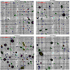 |
Fig. 1. High-contrast greyscale 1 × 1 arcmin R-band images obtained from the MUSE data cubes. The position of each FXT is indicated by a dashed cyan circle near the centre of the image. Its size represents the 1σ uncertainty on the X-ray position of the FXT. Every ellipse indicates the position of a source detected by SEP, with different colours for different types of sources. Green ellipses show sources for which we detected emission lines in the spectra to which we fit Gaussian functions to determine the redshift. Yellow ellipses indicate sources for which we used the Ca H+K absorption lines to estimate a redshift and used PPXF to obtain a more accurate redshift measurement. Orange ellipses indicate sources that were identified as dwarf stars, and pink ellipses show sources that are normal stars. The red ellipses were filtered out by our selection criteria based on flags and elongation. We extracted a spectrum for blue sources, but the signal-to-noise ratio was too low to detect emission lines or use PPXF to obtain the redshift. We note that due to the high contrast of the image needed to show all faint sources, not all sources that appear bright have a high S/N spectrum. We plot the spectrum of the source with an R-band magnitude of 22.76 ± 0.06, marked with a red cross in the image of XRT 070618 in Figure 2 to give an example of a bright source for which we were unable to determine the redshift. The sizes of the ellipses show the extraction region used to obtain the spectrum for each source (see Section 3.3 for how the size and shape were determined). The sources for which we were able to obtain a redshift are labelled with numbers that correspond to the numbers listed in Table A.1. Orange ellipses are labelled with numbers corresponding to the source numbers listed in Table 2. North is up and east is left in these images. |
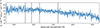 |
Fig. 2. Spectrum of the source with an R-band magnitude of 22.76 ± 0.06, marked with a red cross in the image of XRT 070618 in Figure 1, smoothed using Box1DKernel with a kernel width of 10 pixels to give an example of a bright source for which we were unable to determine the redshift. |
The labelled sources are listed in Table A.1, including the derived redshift (and the line identifications), the absolute and apparent magnitudes, the offset between the FXT and the candidate host galaxy, the corresponding (0.3−10 keV) LX, peak, and the chance alignment probability. For sources for which only one emission line was detected, we opted to identify it as originating from the [OII] doublet, and we accordingly fit this line with two Gaussian functions to account for it being a doublet. An alternative often used assumption is that a single line is due to Hα, but for the spectra where this one line is at wavelengths that are shorter than the rest-frame wavelength of Hα, this is not a valid assumption. For the remaining cases, we base the assumption that this line is [O II] on the absence of other emission lines. For example, most of these single lines have a high signal-to-noise ratio, which means, assuming a typical Balmer decrement of ∼3, that we would, for example, expect to be able to detect the Hβ emission line if this detected line were Hα. For the sources with a higher redshift, the two lines in the doublet are visible as two clearly separate lines, lending support to the doublet identification. We plotted the fits to the [O II] doublets when this line alone was used to determine the redshift in the supplementary material5. However, due to the potential of a large systematic error because of a misidentification in these cases, we report these redshift determinations without an error bar. We plot the spectra of the sources for which we determined the redshift using emission lines in the supplementary material5, where we indicate the position of the emission lines we used. Also in the supplementary material5, we show the best-fitting galaxy found by PPXF, plotted on top of the extracted spectrum when the redshift was determined using the calcium H+K lines and PPXF. The redshift was determined using both methods for eight sources.
For the dwarf stars (orange sources), we used the spectra of M and K dwarfs from the Pickles Stellar Spectral Flux Library Pickles (1998) in combination with PPXF to find the best-fitting stellar type. The best-fitting dwarf star types are listed in Table 2, and the reduced χ2 for the best fit is also included. The best fits to the spectra are shown in the supplementary material5. For the remaining sources that were not categorised as stars, we are unable to obtain a redshift through either emission-line fitting or using PPXF because the signal-to-noise ratio is too low. For completeness, the extracted spectra of the 1σ uncertainty regions are included in the supplementary material5.
Sources per FXT for which we fitted K and M dwarf spectra to the extracted MUSE spectra.
5. Discussion
When we assume that one of the galaxies for which we were able to determine a redshift is the host galaxy of the corresponding FXT LX, peak ≳ 1044 erg s−1 for all cases (Table A.1). Comparing this to the different luminosities expected for different progenitor models, we derive that LX, peak is too high to be produced by the SBO progenitor model for each FXT. Additionally, Figure 1 shows that there are no clear host galaxies within the 3σ X-ray uncertainty position detected in the MUSE data for XRT 030511 and XRT 070618. For XRT 100831, we detect a faint source (mR, AB = 26.5 ± 0.3) within the 1σ uncertainty region, which we discuss below. For XRT 060207 a galaxy lies within the 1σ uncertainty region, which we also discuss below. Additionally, within the 3σ positional uncertainty region of this FXT lie a dwarf star and an object without a redshift determination.
For XRT 030511 and XRT 070618 we did not detect emission lines in the spectra extracted from the 1σ uncertainty positions (see supplementary material5). For XRT 100831 there is suggestive evidence for the detection of an emission line near 8280 Å. We discuss this in more detail below. For XRT 060207 we detect an emission line that we associate with the source found within the 1σ uncertainty region.
For an SBO nature, LX, peak ≲ 1044 erg s−1, so that the maximum redshift for these FXTs to be consistent with the SBO model would be z ∼ 0.12, ∼0.19, ∼0.12, and ∼0.06 for XRT 030511, XRT 100831, XRT 060207 and XRT 070618, respectively. For an SBO, a young massive star is needed, and therefore, we verified whether a star-forming (SF) galaxy, and even an SF dwarf galaxy, can be detected within these upper redshift limits. The typical absolute magnitude of a star-forming (SF) dwarf galaxy is ≳15 in the B band (e.g., Annibali & Tosi 2022). This translates into apparent magnitudes between < 22.3 and < 24.9 for our sample, which we would have (just) been able to detect in the bluer part of the cubes. Unless the SF host galaxy of any of the FXTs is uncharacteristically faint for an SF galaxy, it is unlikely that any of our FXTs stem from SF host galaxies.
When we compare the offsets within our sample of > 33 kpc (1σ limit) to the offset distribution of other types of transients, the offsets we find effectively rule out long gamma-ray bursts (GRBs) (Lyman et al. 2017) and super-luminous SNe (Schulze et al. 2021) natures of the events. The offset distribution of core-collapse SNe (CCNSe) (Kelly & Kirshner 2012; Schulze et al. 2021) is also inconsistent with such a large offset. The types of transients for which a sizeable fraction occurs at > 33 kpc are Type Ia SNe (Uddin et al. 2020) and short GRBs (Fong et al. 2022), which would be consistent with an IMBH-WD TDE (which could lead to thermonuclear explosions similar to Type Ia SNe) and a BNS merger nature of FXTs. In the distribution function of offsets for short GRBs, a fraction of objects has even larger offsets (up until an offset of roughly 100 kpc for the 1% fraction). The 1% limit in the offset distribution function of Type Ias is roughly at 20 to 30 kpc. We stress that it is uncertain whether the FXTs under study are related to any of the candidate host galaxies.
It is uncertain whether globular clusters (GCs) host IMBHs (Bahcall & Ostriker 1975), but they are dense enough to allow for a significant TDE rate (e.g., Fragione et al. 2018). The absolute magnitude distribution of GCs peaks between MV = −7 and MV = −8, depending among other things on the galaxy type (see Rejkuba 2012 for a review), which means that we would not be able to detect GCs around these galaxies for the redshifts we derived. The distribution of galactocentric offsets between GCs and their host galaxies is also not universal. When we take the distributions for the five galaxies discussed in Lomelí-Núñez et al. (2022), hardly any GCs are reported with an offset of > 15 kpc. Therefore, the offsets we report of up to 270 kpc are much larger than expected for GCs (assuming that the distributions of Lomelí-Núñez et al. 2022 are representative for all galaxies). This difference between GC offsets and our offsets could be an argument against an IMBH-WD TDE nature for the FXTs.
5.1. XRT 030511
There are no reliable host galaxy candidates for XRT 030511 based on the offsets and the chance alignment probabilities. We therefore do not discuss the sources listed in Table A.1 in detail for this FXT. When we assume that the faintest source in the R-band image with a significant detection (error < 0.3 mag) is the limiting magnitude of the image, we obtain a limiting magnitude of 26.3. For a typical galaxy with an absolute magnitude of ∼ − 20 (e.g., Chilingarian & Zolotukhin 2012), this implies a redshift of ≳2.2.
5.2. XRT 100831
For XRT 100831 we considered three candidate host spectra in detail. First, Quirola-Vásquez et al. (2022) reported a possible host at 3.2σ of the centre of the uncertainty on the position of XRT 100831. We also detected this source. It lies close to the north-east of the FXT position (marked with a red plus in Figure 1) at 3.3σ. However, we are not able to determine a redshift of this object.
Second, we considered the emission line detected in the spectrum extracted at the location of the FXT, and we fitted two Gaussian functions to this feature based on the assumption that it is due to the [O II] doublet. Using this identification, we obtain a redshift z ∼ 1.22. For this redshift, LX, peak ∼ 8 × 1045 erg s−1, which is too high for an SBO nature. Third, we examined the spectrum of source 21, which falls within the 1σ positional uncertainty of XRT 100831 reported in this work. During our first visual inspection, we discarded this spectrum as we were not certain that the detected line was real (see supplementary material5). However, upon further inspection due to the detection of a line in the spectrum of the position of XRT 100831 we were able to fit lines to the spectrum of source 21, because we had a guess for the redshift from the line of the FXT region spectrum. We find the same redshift of z ∼ 1.22 for source 21, and therefore, we identify the emission line detected in the spectrum extracted from the 1σ uncertainty to have come from this source 21. The projected offset for this source is 6 ± 7 kpc, which is consistent with all three possible progenitor models. This source has a chance alignment probability of 0.04 with the FXT position, so that we consider it likely that this is the host galaxy of XRT 100831.
Sources 48 and 49 of XRT 100831 are both at a redshift of z ∼ 0.324. The average projected offset to the position of XRT 100831 is 120 ± 4 kpc for these two galaxies, and no other sources with a similar redshift are found within the sample of sources with a derived redshift. Another two sources, 24 and 26, lie at a redshift z ∼ 1.01 with an average projected offset to the position of XRT 100831 of 203 ± 7 kpc. For both sets of galaxies, the offset is too large for it to be likely that XRT 100831 originated from either pair.
5.3. XRT 060207
Source 36 is located within the 1σ uncertainty region of XRT 060207. This galaxy has a redshift of 0.939 that was determined through the detection of one emission line identified as the [OII] doublet. While the emission line falls within 16 Å of the skyline at 7246 Å, we consider it a solid detection. If this galaxy is the host of XRT 060207, LX, peak = 1.2 × 1046 erg s−1, which falls within the peak luminosity range of both the BNS and the IMBH-WD TDE progenitor models. The offset at the distance of this galaxy is 14 ± 15 kpc, which is consistent with the offset distribution of all three progenitor models. The chance alignment probability between this galaxy and the FXT is 0.06. Therefore, we consider source 36 a viable host galaxy candidate for XRT 060207.
Another source lies within the 3σ uncertainty region of XRT 060207, source 40. This is identified by us as a type M1V late-type star (see Table 2). The R-band magnitude of this source is 21.27 ± 0.03 magAB. This magnitude is obtained through aperture photometry with SOURCE EXTRACTOR using a circular aperture of 2.5 times the FWHM, where the FWHM was determined with imexam in IRAF. We used this magnitude to calculate log(LX/Lbol) = log(FX/Fbol) following the same procedure as Quirola-Vásquez et al. (2022)6 and find −2.9 ≲ log(FX/Fbol)≲0.1 depending on the spectral type of the synthetic model. The saturation limit of M dwarfs was reported by De Luca et al. (2020) to be as high as log(FX/Fbol)≲0.0, which is consistent with the values we find.
We calculated the chance alignment probability of the FXT position with this late-type star by using the procedure described in Section 3.6, but we determined the surface density of stars brighter than source 40 locally on the image. Ten stars are brighter than source 40 in the image of 1 arcmin2, leading to a chance alignment probability of 0.16 for the distance of 4.2 arcsec between the FXT position and the dwarf star. When we limit our surface density calculation to only include late-type stars, source 40 is the brightest, and the chance alignment probability is 0.02. Compared to the chance alignment probability of the galaxy (source 36) with the FXT position of 0.06, there is no clear best association of the FXT with either of these sources.
For XRT 060207 there is group of galaxies (sources 4, 45, 51, and 55) at z ∼ 0.588. For this group of sources, the projected distance is 156 ± 13 kpc. The positions of these four sources compared to the position of the FXT (three to the north-west and one to the south-west) might indicate that this FXT occurred due to interactions between these galaxies. If the FXT were to belong to this group of galaxies (assuming these galaxies form a group), LX, peak = 3.9 × 1045 erg s−1.
Two sources (25 and 41) lie at z ∼ 0.592. This pair is east of the FXT position, with an average position of XRT 060207 ∼40 kpc away from this FXT position. The average projected offset is consistent with a BNS merger origin.
5.4. XRT 070618
Alp & Larsson (2020) reported two potential host galaxies for XRT 070618, which they assumed to be at the same redshift. The two sources are numbered as source 14 (the galaxy reported at 12 arcsec from the FXT position with mR = 21.16 ± 0.03 magAB) and source 22 (the galaxy at 21 arcsec from the FXT position with mR = 18.86 ± 0.01 magAB) in the bottom right panel of Figure 1 in this work. They fitted the SEDs of both galaxies simultaneously to obtain the redshift of the pair as z = 0.37, which they assumed as the redshift of the FXT. However, we found that these sources are not located at the same redshift, with source 14 located at z = 0.43217(1) and source 22 located at z = 0.20803(9). This results in an LX, peak of 7.5 × 1045 and 1.4 × 1045 erg s−1 assuming either source 14 or source 22 is the host galaxy of XRT 070618. For either of these galaxies, we therefore rule out an SBO nature based on LX, peak > 1044 and the offset of the FXT with respect to these host galaxies.
For XRT 070618 galaxy 3 and 6 lie at approximately the same redshift of z ∼ 0.367. However, the location of XRT 070618 with respect to this galaxy pair at an average projected offset of ∼45 kpc still indicates a progenitor model that is not an SBO due to the offset and LX, peak.
It is possible that none of the candidate host galaxies discussed above is the real host galaxy. For instance, the real host galaxy might be too faint to be detected in our MUSE data. It can be intrinsically faint or appear to be faint due to a large distance. At a limiting magnitude in the R-band images of ∼25 mag (this limiting magnitude is derived from the faintest detected objects), dwarf galaxies such as the Large Magellanic Cloud with an absolute magnitude of MV ∼ −18 could be detected out to a distance of ∼4 Gpc or z ∼ 0.65. For the host galaxy to be undetected at the positions of the FXTs, it therefore either has to be at a larger distance or it has to be fainter than MV ∼ −18 for z < 0.65. If the galaxy is at z > 0.65 LX, peak ≳ 2 × 1045 erg s−1 for all sources.
6. Conclusions
We studied the environment of four FXTs reported by Lin et al. (2019), Alp & Larsson (2020), and Quirola-Vásquez et al. (2022). We reported redshifts for between 13 and 22 galaxies in the images of these FXTs and used these redshifts to constrain LX, peak and the nature of the FXTs. We detected candidate host galaxies for two FXTs. For XRT 100831 we detected an emission line in the spectrum extracted from the 1σ positional uncertainty region. We identified this line as originating from a very faint source within the 1σ positional uncertainty. This source lies at z ∼ 1.22 and has a chance alignment probability of 0.04. The BNS merger model or the IMBH-WD TDE model are both viable progenitors for this FXT based on the peak X-ray luminosity when we assume that this source is the host galaxy of XRT 100831. We consider that this source likely is the host galaxy of XRT 100831.
For XRT 060207, we detect a galaxy at redshift z = 0.939 within the 1σ uncertainty region with a low chance alignment probability. If this is indeed the host galaxy of XRT 060207, the most likely progenitor would either be the BNS merger model or the IMBH-WD TDE model based on the offset and the peak X-ray luminosity. Another source lies within the 3σ uncertainty position, however. This is an M dwarf star with a similar chance alignment probability as the galaxy with the FXT position. With the available data, we cannot determine with which of these two sources XRT 070618 is associated.
All FXTs have LX, peak that are too high and have a large offset with respect to all other candidate host galaxies, so that they are probably not produced by an SN SBO. We cannot distinguish between the other models, IMBH-WD TDE or BNS merger, based on LX, peak and the offsets. We note, however, that for the galaxies with offsets > 30 kpc, an IMBH-WD TDE is unlikely due to the large offset. The question still remains whether all FXTs have the same progenitor or if there are subgroups stemming from different progenitors.
Data availability
Supplementary material is available at https://zenodo.org/records/12805278
This is already happening: during the commissioning phase of the Einstein Probe, EP240315a was reported shortly after its discovery (Zhang et al. 2024).
For an explanation of all the flag values, see https://sextractor.readthedocs.io/en/latest/Flagging.html
In short: we normalize stellar synthetic models of dwarf stars taken from Phillips et al. (2020) (1000 ≲ Teff ≲ 3000 K and 2.5 ≲ log g ≲ 5.5) to the R band magnitude obtained for this star, and integrate the normalised models at optical through NIR wavelengths to calculate the bolometric flux.
Acknowledgments
Based on observations made with ESO Telescopes at the La Silla Paranal Observatory under programme ID 109.236W with PI D. Eappachen. This work is part of the research programme Athena with project number 184.034.002, which is financed by the Dutch Research Council (NWO). This publication is part of the project Dutch Black Hole Consortium (with project number 1292.19.202) of the research programme NWA which is (partly) financed by the Dutch Research Council (NWO). P.G.J. has received funding from the European Research Council (ERC) under the European Union’s Horizon 2020 research and innovation programme (Grant agreement No. 101095973). We acknowledge support from ANID – Millennium Science Initiative Program – ICN12_009 (FEB, JQV), CATA-BASAL – FB210003 (FEB), and FONDECYT Regular – 1200495 (FEB) and 1241005 (FEB). This work makes use of Python packages NUMPY (Harris et al. 2020), SCIPY (Virtanen et al. 2020); MATPLOTLIB (Hunter 2007), PYMUSE Pessa et al. (2018), LMFITNewville et al. (2015) This work made use of Astropy (http://www.astropy.org): a community-developed core Python package and an ecosystem of tools and resources for astronomy (Astropy Collaboration 2013, 2018, 2022).
References
- Alp, D., & Larsson, J. 2020, ApJ, 896, 39 [NASA ADS] [CrossRef] [Google Scholar]
- Ambruster, C. W., & Wood, K. S. 1986, ApJ, 311, 258 [NASA ADS] [CrossRef] [Google Scholar]
- Annibali, F., & Tosi, M. 2022, Nat. Astron., 6, 48 [NASA ADS] [CrossRef] [Google Scholar]
- Arefiev, V. A., Priedhorsky, W. C., & Borozdin, K. N. 2003, ApJ, 586, 1238 [NASA ADS] [CrossRef] [Google Scholar]
- Astropy Collaboration (Robitaille, T. P., et al.) 2013, A&A, 558, A33 [NASA ADS] [CrossRef] [EDP Sciences] [Google Scholar]
- Astropy Collaboration (Price-Whelan, A. M., et al.) 2018, AJ, 156, 123 [Google Scholar]
- Astropy Collaboration (Price-Whelan, A. M., et al.) 2022, ApJ, 935, 167 [NASA ADS] [CrossRef] [Google Scholar]
- Bahcall, J. N., & Ostriker, J. P. 1975, Nature, 256, 23 [NASA ADS] [CrossRef] [Google Scholar]
- Barbary, K. 2016, J. Open Source Softw., 1, 58 [Google Scholar]
- Bauer, F. E., Treister, E., Schawinski, K., et al. 2017, MNRAS, 467, 4841 [NASA ADS] [CrossRef] [Google Scholar]
- Berger, E. 2014, ARA&A, 52, 43 [CrossRef] [Google Scholar]
- Bertin, E., & Arnouts, S. 1996, A&AS, 117, 393 [NASA ADS] [CrossRef] [EDP Sciences] [Google Scholar]
- Bloom, J. S., Kulkarni, S. R., & Djorgovski, S. G. 2002, AJ, 123, 1111 [NASA ADS] [CrossRef] [Google Scholar]
- Cappellari, M. 2017, MNRAS, 466, 798 [Google Scholar]
- Castro-Tirado, A. J., Brandt, S., Lund, N., & Sunyaev, R. 1999, A&A, 347, 927 [NASA ADS] [Google Scholar]
- Chilingarian, I. V., & Zolotukhin, I. Y. 2012, MNRAS, 419, 1727 [Google Scholar]
- Cold, C., & Hjorth, J. 2023, A&A, 670, A48 [NASA ADS] [CrossRef] [EDP Sciences] [Google Scholar]
- Connors, A., Serlemitsos, P. J., & Swank, J. H. 1986, ApJ, 303, 769 [NASA ADS] [CrossRef] [Google Scholar]
- Dai, L., McKinney, J. C., Roth, N., Ramirez-Ruiz, E., & Miller, M. C. 2018, ApJ, 859, L20 [Google Scholar]
- De Luca, A., Stelzer, B., Burgasser, A. J., et al. 2020, A&A, 634, L13 [NASA ADS] [CrossRef] [EDP Sciences] [Google Scholar]
- Eappachen, D., Jonker, P. G., Fraser, M., et al. 2022, MNRAS, 514, 302 [NASA ADS] [CrossRef] [Google Scholar]
- Eappachen, D., Jonker, P. G., Levan, A. J., et al. 2023, ApJ, 948, 91 [NASA ADS] [CrossRef] [Google Scholar]
- Eappachen, D., Jonker, P. G., Quirola-Vásquez, J., et al. 2024, MNRAS, 527, 11823 [Google Scholar]
- Fong, W.-F., Nugent, A. E., Dong, Y., et al. 2022, ApJ, 940, 56 [NASA ADS] [CrossRef] [Google Scholar]
- Fragione, G., Leigh, N. W. C., Ginsburg, I., & Kocsis, B. 2018, ApJ, 867, 119 [NASA ADS] [CrossRef] [Google Scholar]
- Frei, Z., & Gunn, J. E. 1994, AJ, 108, 1476 [NASA ADS] [CrossRef] [Google Scholar]
- García-Alvarez, D., Drake, J. J., Kashyap, V. L., Lin, L., & Ball, B. 2008, ApJ, 679, 1509 [CrossRef] [Google Scholar]
- Glennie, A., Jonker, P. G., Fender, R. P., Nagayama, T., & Pretorius, M. L. 2015, MNRAS, 450, 3765 [NASA ADS] [CrossRef] [Google Scholar]
- Goldberg, J. A., Jiang, Y.-F., & Bildsten, L. 2022, ApJ, 933, 164 [NASA ADS] [CrossRef] [Google Scholar]
- Hakobyan, A. A., Adibekyan, V. Z., Aramyan, L. S., et al. 2012, A&A, 544, A81 [NASA ADS] [CrossRef] [EDP Sciences] [Google Scholar]
- Harris, C. R., Millman, K. J., van der Walt, S. J., et al. 2020, Nature, 585, 357 [NASA ADS] [CrossRef] [Google Scholar]
- Hogg, D. W., Pahre, M. A., McCarthy, J. K., et al. 1997, MNRAS, 288, 404 [NASA ADS] [CrossRef] [Google Scholar]
- Hunter, J. D. 2007, Comput. Sci. Eng., 9, 90 [NASA ADS] [CrossRef] [Google Scholar]
- Jonker, P. G., Heida, M., Torres, M. A. P., et al. 2012, ApJ, 758, 28 [NASA ADS] [CrossRef] [Google Scholar]
- Jonker, P. G., Glennie, A., Heida, M., et al. 2013, ApJ, 779, 14 [NASA ADS] [CrossRef] [Google Scholar]
- Kelly, P. L., & Kirshner, R. P. 2012, ApJ, 759, 107 [NASA ADS] [CrossRef] [Google Scholar]
- Kron, R. G. 1980, ApJS, 43, 305 [Google Scholar]
- Lai, D., Wang, C., & Han, J. 2006, Chin. J. Astron. Astrophys. Suppl., 6, 241 [NASA ADS] [CrossRef] [Google Scholar]
- Lin, D., Irwin, J., & Berger, E. 2019, ATel, 13171 [Google Scholar]
- Lin, D., Irwin, J. A., Berger, E., & Nguyen, R. 2022, ApJ, 927, 211 [NASA ADS] [CrossRef] [Google Scholar]
- Lomelí-Núñez, L., Mayya, Y. D., Rodríguez-Merino, L. H., Ovando, P. A., & Rosa-González, D. 2022, MNRAS, 509, 180 [Google Scholar]
- Lyman, J. D., Levan, A. J., Tanvir, N. R., et al. 2017, MNRAS, 467, 1795 [NASA ADS] [Google Scholar]
- MacLeod, M., Guillochon, J., Ramirez-Ruiz, E., Kasen, D., & Rosswog, S. 2016, ApJ, 819, 3 [NASA ADS] [CrossRef] [Google Scholar]
- Merritt, D., Schnittman, J. D., & Komossa, S. 2009, ApJ, 699, 1690 [NASA ADS] [CrossRef] [Google Scholar]
- Newville, M., Stensitzki, T., Allen, D. B., & Ingargiola, A. 2015, https://doi.org/10.5281/zenodo.11813 [Google Scholar]
- Novara, G., Esposito, P., Tiengo, A., et al. 2020, ApJ, 898, 37 [Google Scholar]
- Pessa, I., Tejos, N., & Moya, C. 2018, ArXiv e-prints [arXiv:1803.05005] [Google Scholar]
- Phillips, M. W., Tremblin, P., Baraffe, I., et al. 2020, A&A, 637, A38 [NASA ADS] [CrossRef] [EDP Sciences] [Google Scholar]
- Pickles, A. J. 1998, PASP, 110, 863 [NASA ADS] [CrossRef] [Google Scholar]
- Planck Collaboration XIII. 2016, A&A, 594, A13 [NASA ADS] [CrossRef] [EDP Sciences] [Google Scholar]
- Pradhan, A. K., Montenegro, M., Nahar, S. N., & Eissner, W. 2006, MNRAS, 366, L6 [NASA ADS] [CrossRef] [Google Scholar]
- Quirola-Vásquez, J., Bauer, F. E., Jonker, P. G., et al. 2022, A&A, 663, A168 [NASA ADS] [CrossRef] [EDP Sciences] [Google Scholar]
- Quirola-Vásquez, J., Bauer, F. E., Jonker, P. G., et al. 2023, A&A, 675, A44 [NASA ADS] [CrossRef] [EDP Sciences] [Google Scholar]
- Quirola-Vásquez, J., Bauer, F. E., Jonker, P. G., et al. 2024, A&A, 683, A243 [NASA ADS] [CrossRef] [EDP Sciences] [Google Scholar]
- Reines, A. E., Greene, J. E., & Geha, M. 2013, ApJ, 775, 116 [Google Scholar]
- Rejkuba, M. 2012, Ap&SS, 341, 195 [Google Scholar]
- Schulze, S., Yaron, O., Sollerman, J., et al. 2021, ApJS, 255, 29 [NASA ADS] [CrossRef] [Google Scholar]
- Soderberg, A. M., Berger, E., Page, K. L., et al. 2008, Nature, 453, 469 [NASA ADS] [CrossRef] [Google Scholar]
- Soto, K. T., Lilly, S. J., Bacon, R., Richard, J., & Conseil, S. 2016, MNRAS, 458, 3210 [Google Scholar]
- Uddin, S. A., Burns, C. R., Phillips, M. M., et al. 2020, ApJ, 901, 143 [NASA ADS] [CrossRef] [Google Scholar]
- Vazdekis, A., Sánchez-Blázquez, P., Falcón-Barroso, J., et al. 2010, MNRAS, 404, 1639 [NASA ADS] [Google Scholar]
- Virtanen, P., Gommers, R., Oliphant, T. E., et al. 2020, Nat. Meth., 17, 261 [Google Scholar]
- Waxman, E., & Katz, B. 2017, in Handbook of Supernovae, eds. A. W. Alsabti, & P. Murdin, 967 [CrossRef] [Google Scholar]
- Webb, N. A., Coriat, M., Traulsen, I., et al. 2020, A&A, 641, A136 [NASA ADS] [CrossRef] [EDP Sciences] [Google Scholar]
- Weilbacher, P. M., Palsa, R., Streicher, O., et al. 2020, A&A, 641, A28 [NASA ADS] [CrossRef] [EDP Sciences] [Google Scholar]
- Xue, Y. Q., Zheng, X. C., Li, Y., et al. 2019, Nature, 568, 198 [NASA ADS] [CrossRef] [Google Scholar]
- Yuan, W., Zhang, C., Chen, Y., & Ling, Z. 2022, in Handbook of X-ray and Gamma-ray Astrophysics, eds. C. Bambi, & A. Santangelo, 86 [Google Scholar]
- Zhang, W. J., Mao, X., Zhang, W. D., et al. 2024, GRB Coordinates Network, 35931 [Google Scholar]
Appendix A: Additional table after the references
Sources per FXT for which we extracted spectra from the MUSE cubes, according to the selection criteria explained in Section 3.2.
All Tables
Sources per FXT for which we fitted K and M dwarf spectra to the extracted MUSE spectra.
Sources per FXT for which we extracted spectra from the MUSE cubes, according to the selection criteria explained in Section 3.2.
All Figures
|
Fig. 1. High-contrast greyscale 1 × 1 arcmin R-band images obtained from the MUSE data cubes. The position of each FXT is indicated by a dashed cyan circle near the centre of the image. Its size represents the 1σ uncertainty on the X-ray position of the FXT. Every ellipse indicates the position of a source detected by SEP, with different colours for different types of sources. Green ellipses show sources for which we detected emission lines in the spectra to which we fit Gaussian functions to determine the redshift. Yellow ellipses indicate sources for which we used the Ca H+K absorption lines to estimate a redshift and used PPXF to obtain a more accurate redshift measurement. Orange ellipses indicate sources that were identified as dwarf stars, and pink ellipses show sources that are normal stars. The red ellipses were filtered out by our selection criteria based on flags and elongation. We extracted a spectrum for blue sources, but the signal-to-noise ratio was too low to detect emission lines or use PPXF to obtain the redshift. We note that due to the high contrast of the image needed to show all faint sources, not all sources that appear bright have a high S/N spectrum. We plot the spectrum of the source with an R-band magnitude of 22.76 ± 0.06, marked with a red cross in the image of XRT 070618 in Figure 2 to give an example of a bright source for which we were unable to determine the redshift. The sizes of the ellipses show the extraction region used to obtain the spectrum for each source (see Section 3.3 for how the size and shape were determined). The sources for which we were able to obtain a redshift are labelled with numbers that correspond to the numbers listed in Table A.1. Orange ellipses are labelled with numbers corresponding to the source numbers listed in Table 2. North is up and east is left in these images. |
| In the text | |
|
Fig. 2. Spectrum of the source with an R-band magnitude of 22.76 ± 0.06, marked with a red cross in the image of XRT 070618 in Figure 1, smoothed using Box1DKernel with a kernel width of 10 pixels to give an example of a bright source for which we were unable to determine the redshift. |
| In the text | |
Current usage metrics show cumulative count of Article Views (full-text article views including HTML views, PDF and ePub downloads, according to the available data) and Abstracts Views on Vision4Press platform.
Data correspond to usage on the plateform after 2015. The current usage metrics is available 48-96 hours after online publication and is updated daily on week days.
Initial download of the metrics may take a while.