| Issue |
A&A
Volume 685, May 2024
|
|
|---|---|---|
| Article Number | L7 | |
| Number of page(s) | 7 | |
| Section | Letters to the Editor | |
| DOI | https://doi.org/10.1051/0004-6361/202449877 | |
| Published online | 07 May 2024 | |
Letter to the Editor
Spectroscopic evidence of a possible young stellar cluster at the Galactic Center
1
Instituto de Astrofísica de Andalucía (CSIC), University of Granada, Glorieta de la astronomía s/n, 18008 Granada, Spain
e-mail: amartinez@iaa.es
2
European Southern Observatory, Karl-Schwarzschild-Strasse 2, 85748 Garching bei München, Germany
3
Centro de Astrobiología (CSIC/INTA), ctra. de Ajalvir km. 4, 28850 Torrejón de Ardoz, Madrid, Spain
Received:
6
March
2024
Accepted:
22
April
2024
Context. The nuclear stellar disk has been the most prolific star-forming region in the Milky Way over the past ∼30 million years. Notably, the cumulative mass of the three clusters currently found in the nuclear stellar disk, the Quintuplet, the Arches, and the Nuclear clusters, amounts to just 10% of the total anticipated mass of young stars that formed in this period. This discrepancy, known as the missing cluster problem, is attributed to factors such as high stellar density and tidal forces. Traces of dissolving clusters may exist as comoving groups of stars, providing insights into the star formation history of the region. Recently, a new cluster candidate associated with an HII region was reported through the analysis of kinematic data
Aims. Our aim is to determine whether the young and massive stellar objects in the region share proper motion, positions in the plane of the sky, and line-of-sight distances. We use reddening as a proxy for the distances.
Methods. We reduced and analyzed integral field spectroscopy data from the KMOS instrument at the ESO VLT to locate possible massive young stellar objects in the field. Then, we identified young massive stars with astrophotometric data from the two different catalogs to analyze their extinction and kinematics.
Results. We present a group of young stellar objects that share velocities, are close together in the plane of the sky, and are located at a similar depth in the nuclear stellar disk.
Conclusions. The results presented here offer valuable insights into the missing clusters problem. They indicate that not all young massive stars in the Galactic center form in isolation; some of them seem to be the remnants of dissolved clusters or stellar associations.
Key words: proper motions / Galaxy: nucleus / Galaxy: structure
© The Authors 2024
 Open Access article, published by EDP Sciences, under the terms of the Creative Commons Attribution License (https://creativecommons.org/licenses/by/4.0), which permits unrestricted use, distribution, and reproduction in any medium, provided the original work is properly cited.
This article is published in open access under the Subscribe to Open model. Subscribe to A&A to support open access publication.
1. Introduction
The Galactic center (GC) is located at a distance of ∼ 8.25 kpc (GRAVITY Collaboration 2020) and harbors the nuclear stellar disk (NSD). This flat rotating structure (Schonrich et al. 2015; Shahzamanian et al. 2022) spans about 150 pc across and has a scale height of 40 pc (Launhardt et al. 2002; Sormani et al. 2022). With a star formation rate of ∈[0.2 − 0.8] M⊙ yr−1 over the past 30 Myr (Matsunaga et al. 2011; Nogueras-Lara et al. 2020), the NSD stands out as the most prolific star-forming region of the Galaxy when averaged over volume. This contrasts with the number of star clusters currently known in the NSD, namely the Arches and Quintuplet clusters, which account for a few percent of this mass at most. This discrepancy, known as the missing clusters problem, can be attributed to the challenging conditions in the GC, including substantial and varying extinction (Nishiyama et al. 2009; Nogueras-Lara et al. 2019b), which limit observations to the near-infrared, making the identification of young stars very challenging. Clusters in this environment dissolve in ≲10 Myr (Kim et al. 1999; Portegies Zwart et al. 2001; Kruijssen et al. 2014), and color-magnitude diagrams are dominated by reddening, making them a poor tool for cluster identification (Nogueras-Lara et al. 2018). However, recent studies found substantial masses of young stars in Sgr B1 and Sgr C (Nogueras-Lara et al. 2022; Nogueras-Lara 2024), supporting coeval formation followed by rapid dissolution in the NSD.
Identifying young stellar associations via spectroscopy is feasible, but is constrained by the limited field of view and time requirements. It is impractical to cover the entire NSD with spectroscopic surveys, but specific areas can be targeted by identifying comoving groups (Shahzamanian et al. 2019; Martínez-Arranz et al. 2024). This two-step approach involves first identifying comoving groups and then confirming the presence of young massive stars through spectroscopy to uncover previously undetected clusters or associations.
A comoving group is characterized as a set of stars whose members are close in space and share similar velocities, exhibiting a velocity dispersion lower than that of other stars in the field. It can be defined by a 6D parameter space, three dimensions for the velocity components, and three for the position components. While the available catalogs for the GC only provide positions and proper motions in the plane of the sky, the third dimension in position, the line-of-sight distance, can indirectly be constrained by using observed stellar colors. Given the substantial extinction variability in the NSD (Nogueras-Lara et al. 2021b; Shahzamanian et al. 2022; Nogueras-Lara 2022) and the almost constant intrinsic colors of observable stars, with variations H − Ks color ≲0.01 mag (see Fig. 33 in Nogueras-Lara et al. 2018), we propose that the alterations in color primarily result from extinction (see also Nogueras-Lara et al. 2021b). Therefore, a group of stars exhibiting similar colors likely shares a comparable depth within the NSD (Nogueras-Lara 2022).
If a comoving group is indeed the remnant of a cluster or a stellar association and is now in the process of dissolution, its member stars should still be relatively young, with ages of about ≲10 Myr. Massive young stars (MYSs) can be separated from cool late-type stars via an analysis of the spectral CO and Brγ lines in the near-infrared (Paumard et al. 2006; Habibi et al. 2019). Cool late-type stars present the 12CO(2,0), 12CO(3,1), and 12CO(4,2) bandhead absorptions at 2.30, 2.33, and 2.35 μm, respectively. Young hot massive stars do not show these features and occasionally present an emission or absorption Brγ line at 2.16 μm and/or HeI abortion at 2.06 μm.
A comoving group was reported in Shahzamanian et al. (2019). This group was found in a known HII-emitting area (Dong et al. 2017), with the presence of a strong Paschen-α emitting star (Dong et al. 2011; Clark et al. 2021), making this region a solid candidate for hosting MYSs. Subsequently, we collected spectroscopy data of this regions. Here, we analyze the spectra of the objects in the area centered in the comoving group and select the MYSs based on the analysis of their spectra. Finally, we cross-match these objects with two different catalogs: the GALACTICNUCLUES survey (Nogueras-Lara et al. 2018, 2019a) and the proper motion catalog by Libralato et al. (2021), to obtain photometry and proper motions.
2. Data and methods
2.1. Spectroscopy data
We acquired infrared field spectroscopy data with the Very Large Telescope (VLT) K-band Multi Object Spectrograph (KMOS) at the European Southern Observatory (ESO), under ESO program ID 105.20CN.0011. KMOS (Sharples et al. 2013) is equipped with 24 integral field units (IFUs), each offering a field of view of 2.8 by 2.8 arcsec (red square in Fig. 1). The observations were conducted in MOSAIC mode, where the individual IFUs of the 24 arms are arranged in such a way that with 16 successive telescope pointings, a contiguous rectangular area can be covered (dashed line in Fig. 1). With all 24 IFUs and 16 pointings, it is possible to map an area of ∼0.8 arcmin2. In order to eliminate the infrared emission from the atmosphere, we needed to acquire images of an area of the sky that was relatively free of stars. Typically, these images are obtained by jittering the science observations. However, due to the crowded environment of the GC, the sky observations cannot be obtained from the jittered observations of the target field. Thus, we used a separate field centered on a dark cloud in the GC as the sky (Table 1).
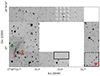 |
Fig. 1. KMOS field of view. The colored triangles depict identified MYSs with a K magnitude brighter than 14.5. The size of each point is proportional to its magnitude. The red square represents the area covered by a single IFU. The dashed black square represents the area covered by a single IFU after completing an observational sequence in the MOSAIC mode (16 pointings). The solid black box indicates the size of the fields into which we divided the image to be able to align them with the GC catalogs. |
KMOS observation parameters.
We reduced the data using the EsoReflex KMOS pipeline (version 3.0.1, Freudling et al. 2013) using the standard recipes provided by ESO. To correct for atmospheric absorption, we used molecfit (Smette et al. 2015) on a standard star spectrum. The default configuration fits a polynomial to eight intervals, from 1.975 to 2.475 μm. Simultaneous fitting of all eight intervals degrades the quality of the corrections for atmospheric absorption at the shortest and longest wavelengths. To improve this, we divided the intervals into three overlapping groups (1.975–2.291 μm, 2.269–2.379 μm, and 2.360–2.475 μm), ran molecfit separately for each group, and then combined the results.
2.2. Astrophotometry data
To provide precise astrometric information for the objects in the KMOS image, we conducted a cross match with two different catalogs: the GALACTICNUCLEUS survey (hereafter GNS) (Nogueras-Lara et al. 2018, 2019a), and the 2D proper motion catalog by Libralato et al. (2021, hereafter L21). The combined dataset from these two catalogs is referred to as GNS-L21.
2.2.1. GNS
GNS is a near-infrared survey (J, H, and Ks bands) covering an area of approximately 6000 pc2 in the GC with an angular resolution of 0.2″. This high spatial resolution is achieved through the application of holographic imaging techniques (Schödel et al. 2013). GNS delivers highly precise PSF photometry for over three million stars in the NSD and inner Galactic bar. In order to eliminate foreground stars belonging to the spiral arms and the bulge, we applied a color cut H − Ks > 1.3 (see Fig. 6 in Nogueras-Lara et al. 2021a). For more details about the GNS, we refer to Nogueras-Lara et al. (2018) and Nogueras-Lara et al. (2019a)
2.2.2. L21
We used L21 to provide the stars observed with KMOS with proper motion values. This catalog resulted from two observation sets covering approximately 205 arcmin2 (see Fig. 1 Libralato et al. 2021). These observations, performed in October 2012 and August 2015, used the near-infrared channel of the Wide-Field Camera 3 (WFC3) on the Hubble Space Telescope (HST). Proper motions were calibrated with reference to Gaia DR2 (Gaia Collaboration 2016), yielding absolute proper motion measurements for around 830 000 stars. We trimmed the catalog by discarding stars with proper motion errors exceeding 1 mas yr−1. For detailed information on data acquisition, reduction, and analysis, we refer to Libralato et al. (2021) 2.
2.3. Methods
The analysis of the data was divided into two distinct stages: First, we extracted spectra from the objects in the field of view from the KMOS data cubes, and second, we identified these sources in the GNS-L21 catalog.
In the initial stage, we extracted spectra for approximately 300 stars and classified them into two categories: late-type stars or MYS. Our primary criterion was the presence of CO bandhead absorption, which is characteristic of asymptotic giant branch stars and late-type G, K, M giants (Schultheis et al. 2003; Nandakumar et al. 2018). To identify MYSs, we selected objects whose spectra did not exhibit any detectable CO absorption.
We extracted the spectra using an aperture of 0.5 arcsec, corresponding to the full width at half maximum of the standard stars used for calibration in the KMOS pipeline. We performed background subtraction from a ring with a radius of twice the full width at half maximum and a width 0.2 arcsec around each object to eliminate any Brγ interstellar emission, which is pervasive in the GC. We customized the background subtraction to avoid using bad pixels or pixels with strong stellar emission.
To estimate the signal-to-noise ratio (S/N) in the MYSs, we selected wavelength intervals in the spectra without any obvious lines and calculated the S/R as the ratio of the mean and standard deviation of the continuum. To ensure that we selected reliable spectra with a clearly distinguished level of the continuum from the background and for which we can determine with certainty that no CO lines were present, we classified as MYSs only stars that without these lines had an S/R > 15. This threshold corresponds to stars whose continuum level is at least twice higher than that of the sky. In our context, this applies to stars brighter than Ks ∼ 14.5. In Fig. 2, we display the spectra of the MYSs with magnitudes brighter than Ks = 14.5. They are color-coded as in Fig. 1.
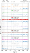 |
Fig. 2. Spectra of the MYSs. The MYSs are color-coded as in Figs. 1 and 3. In blue we show for comparison late-type spectra from stars in the field of approximately the same magnitude as the MYSs. |
In the second part of the analysis, we identified the objects in the KMOS field within the GNS-L21 catalog, enabling us to assign proper motions and H and Ks magnitudes. A significant misalignment issue was present in the 16 pointings necessary for a single IFU to complete an entire tile in mosaic mode (indicated by the dashed black square in Fig. 1). Specifically, notable misalignment was observed between the first eight and the last eight pointings at most IFUs. To compensate for this, we divided the KMOS field into subfields, each encompassing eight consecutive pointings (approximately 15 arcsec2), where consistent IFU alignment was maintained (black box in Fig. 1). Using the astroalign Python package (Beroiz et al. 2020) and dedicated scripts, we cross-matched objects in these parcels with those in the catalogs. Almost all the objects identified in the KMOS field of view, including the seven identified MYSs, had counterparts in the GNS-L21 catalog.
3. Results
We display the identified MYSs in the KMOS image with counterparts in the GNS-L21 catalog in the left and central panels of Fig. 3. We called this group Candela 1, and we refer to it as Can1 throughout. The triangles represents Can1 members, color-coded as in Figs. 1 and 2. The estimated stellar types, coordinates, proper motions, and magnitudes of the Can1 member are shown in Table 2.
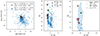 |
Fig. 3. KMOS object proper motions and CMD, and cluster simulation. The triangles represent Can1, and the blue circles represent the remaining objects in the field. Left: vector-point diagram. Middle: CMD. The vertical dashed line marks the color-cut we made to exclude foreground stars (H − Ks = 1.3). The horizontal dashed line marks the magnitude cut we made to exclude stars with low spectroscopic S/R (Ks = 14.5). Right: Spisea cluster simulation. The blue crosses represent members of a simulated cluster. The legend box displays the main features of the cluster. The shaded area represents the uncertainty in the position in the CMD for the members of the simulated cluster due to variations in extinction. |
Parameters of Candela 1 members.
In the left panel of Fig. 3, we show a vector-point diagram of their equatorial proper motions, and the middle panel shows a CMD. Notably, in the left panel of Fig. 3, the velocity dispersion of Can1 is significantly lower than the one corresponding to the remaining stars in the field. In the middle panel, we observe that all Can1 members display a similar color, indicating that they are affected by similar extinction. This supports the idea that these stars are located at a similar depth in the NSD. The similar values in velocity, position in the sky, line-of-sight distance, and the fact that all seven members are massive young stars strongly indicates that this group shares a common origin. Moreover, this group is situated within an HII region (Dong et al. 2017), displaying significant Brγ emission, as illustrated Fig. A.1. This provides additional evidence for recent in situ star formation (Hankins et al. 2019).
If Can1 is part of a larger cluster or stellar association, we can estimate its mass by comparing it with simulated clusters. The Python package Spisea (Hosek et al. 2020) allows the generation of single-age, single-metallicity clusters, and we used it to create models for a comparison with Can1. To generate a cluster model, we needed to set several parameters as input for Spisea: distance, extinction, initial mass function (IMF), age, and metallicity. We adopted a distance of 8.25 kpc (GRAVITY Collaboration 2020). We obtained the extinction value for each star in Can1 from the catalog provided by Nogueras-Lara et al. (2021b). Estimating a single value for the remaining variables was challenging with the current data set. We therefore ran a series of simulations with various combinations. For the ages, we selected four different values ranging from 2.5 Myr, which is the age of the youngest cluster in the NSD, the Arches (Espinoza et al. 2009), to 10 Myr, which is the maximum estimated dissolving time for a massive cluster in the GC (Kim et al. 1999; Kruijssen et al. 2014). For the metalicity, we considered [M/H] = 0 and [M/H] = 0.3 (Najarro et al. 2004; Nogueras-Lara et al. 2020; Schultheis et al. 2021; Feldmeier-Krause 2022). Additionally, we used two different IMFs: a broken power law derived by Kroupa (2001), and a top-heavy one derived by Hosek et al. (2019). This resulted in a total of 16 possible configurations, each run 400 times, producing a total of 6400 simulations.
For each of these simulations, we defined a magnitude interval to compare the model with Can1, using the brighter and fainter magnitudes of Can1. Then, we randomly assigned either a very low or a very high initial mass to the model and compared the number of stars in the magnitude interval with the number of stars in the Can1. If the number of stars in this interval differed from the number of stars in the Can1, we adjusted the mass of the cluster by either increasing or decreasing it. This process was repeated, and the mass was gradually adjusted with ±1% increments until the number of stars in the magnitude interval for the model equaled the number of stars in Can1. Due to completeness limitations, this method only allowed us to estimate a lower limit for the parent cluster of the comoving group, yielding a value of Mestimated = 1742 ± 761 M⊙. In Fig. 3 right panel, we present the CMD of one of these 6400 simulated models alongside the real values of Can1 for comparison.
To investigate the probability of finding a group of seven stars classified as MYSs with a velocity dispersion as low as that of Can1 formed purely by a random association of stars in the field, we conducted a permutation test. We found that the probability of a random association of stars exhibiting similar dynamical characteristics is lower than 0.4%. For more details, we refer to Appendix B.
Determining the radial velocities (vr) of the stars in the comoving group poses challenges due to the featureless spectra they exhibit, in addition to the maximum observation resolution of approximately 30 km s−1. Nevertheless, stars M2 and M3 present a sufficiently intense Brγ absorption line and a sufficiently high S/R to facilitate a rough estimation of the vr. We conducted a Gaussian fitting of the Brγ line, measuring the shift of the line peak relative to the value at rest (Brγ = 2.16612 μm). Subsequently, we applied the barycentric correction to the measured velocity and expressed it in the local standard of rest of the reference frame. We obtained consistent values for the velocities of these two MYSs, M2 with vr ≈ −40 km s−1, and M3 with vr ≈ −50 km s−1.
Finally, we estimated the stellar types for Can1 members by comparing the extracted spectra with the near-infrared spectral atlas provided by Hanson et al. (2005). The estimated classes are presented in the first column of Table 2. For star M1, previous studies by Dong et al. (2011) classified it as an O4-6I (star ID P114 in the reference paper), while Clark et al. (2021) classified it as O4-5Ia+. Both classifications align with the one derived in this study, O4If. For the remaining stars, the estimated types range from O6V to B0-1. The classification of the two faintest stars in the group is challenging due to the limited S/R and the constraint of having only Ks-band data.
We can constrain the age of Can1 by considering the lifespan of its more massive members, the O-type stars. For an O-type star, the maximum age range is approximately 5–6 Myr (Weidner & Vink 2010), which imposes an upper limit for the age of the cluster. This age limit falls within the maximum age of ≲10 Myr that a cluster can survive in the GC before complete dissolution (Kim et al. 1999; Portegies Zwart et al. 2001; Kruijssen et al. 2014).
It is worth mentioning that most of the stars in Can1 presented here have counterparts in a recently identified comoving group by Martínez-Arranz et al. (2024) (Fig. C.1), and it partially overlaps with the one reported by Shahzamanian et al. (2019). Notably, these two comoving groups were identified using different catalogs and methods.
4. Discussion and conclusion
Shahzamanian et al. (2019) reported on a group of seven comoving stars that might be associated with the GC H1 HII region, which is located at a projected distance of only about 11 pc from Sagittarius A* (see, e.g., Dong et al. 2017; Hankins et al. 2019), and with a strong Paschen-α emitting star, the O super-/hyperrgiant P114 (Dong et al. 2011; Clark et al. 2021). Subsequently, Martínez-Arranz et al. (2024) exploited the HST WFC3 proper motion catalog of Libralato et al. (2021) and found a group of 110 comoving stars associated with P114 (ID14966 in Libralato et al. 2021), which may indicate the presence of a young cluster of a few thousand solar masses. The comoving group identified in Shahzamanian et al. (2019) has elements in common with the group reported by Martínez-Arranz et al. (2024).
We presented spectroscopic observations of an area associated with this potential cluster or stellar association. We assigned proper motions and magnitudes to approximately 300 stars, about one-third of which had a sufficiently high S/R to classify them as late-type giants or early-type massive young stars. We found seven young massive stars, including P114. Five of these stars lie within a radius of ∼5″ at a projected distance (about 0.20 pc at the distance of the GC) of P114, and the sixth star lies at ∼15″ (0.60 pc) (Fig. 1). The massive young stars lie very close to each other in the proper motion diagram (left panel in Fig. 3). We called this group Candela 1 (Can1). Furthermore, all star in Can1 have the same HKs colors within the uncertainties, which supports the idea that they also lie close to each other along the line of sight (central panel in Fig. 3). It is worth noting that Can1 is situated very closely to the more probable orbit for the Arches cluster as derived by Hosek et al. (2022) (see also Fig. 1 in Martínez-Arranz et al. 2024). Additionally, the projected distance from the Arches, approximately 20 pc, aligns well with the tidal tail simulation presented in Habibi et al. (2014). Considering these coincidences, the possibility that Can1 may represent traces of a tidal tail associated with the Arches cluster cannot be ruled out. Deeper and more comprehensive observations of the area are necessary to cover the unobserved areas around the main group and acquire spectra with higher S/R, enabling us to classify fainter sources.
Based on these results and on the coexistence with an HII region in the plane of the sky, the evidence is now sufficiently strong to consider Can1 as a newly discovered young cluster at the GC. While we have for several decades known only three young clusters in the GC (Arches, Quintuplet, and the central parsec) plus a few hundred known massive stars distributed throughout the field (Clark et al. 2021), proper motion studies of the GC are now sufficiently precise and complete that we can determine potential clusters via kinematics and then confirm them spectroscopically. This opens a new window into studying star formation in this unique astrophysical environment. Only ≲5% of the area of the NSD has been exploited with this method, and only one candidate cluster was confirmed spectroscopically so far. This suggests that we may still be able to discover a dozen or more new clusters. All of of them will probably be younger than ∼10 Myr because significantly older clusters are expected to have dissolved (Kim et al. 1999; Kruijssen et al. 2014). After having found these new clusters, we will be able to study them in more detail. The perhaps most important question to address will be whether the IMF at the GC is indeed different from the Galactic disk, as indicated by the observations of the three known clusters and as also motivated by theoretical considerations (e.g. Morris 1993; Bartko et al. 2010; Hußmann et al. 2012; Hosek et al. 2019).
The proper motions catalogs are available at https://academic.oup.com/mnras/article/500/3/3213/5960177
Acknowledgments
A. Martínez-Arranz and R. Schödel acknowledge financial support from the Severo Ochoa grant CEX2021-001131-S funded by MCIN/AEI/ 10.13039/501100011033 and support from the State Agency for Research of the Spanish MCIU through the “Center of Excellence Severo Ochoa” award for the Instituto de Astrofísica de Andalucía (SEV-2017-0709). A. Martínez-Arranz and R. Schödel acknowledge support from grant EUR2022-134031 funded by MCIN/AEI/10.13039/501100011033 and by the European Union NextGenerationEU/PRTR. and by grant PID2022-136640NB-C21 funded by MCIN/AEI 10.13039/501100011033 and by the European Union. R.F. acknowledges support from the grants Juan de la Cierva FJC2021-046802-I, PID2020-114461GB-I00 and CEX2021-001131-S funded by MCIN/AEI/10.13039/501100011033 and by “European Union NextGenerationEU/PRTR” and grant P20-00880 from the Consejería de Transformación Económica, Industria, Conocimiento y Universidades of the Junta de Andalucía. We express our gratitude to the referees for their valuable comments and suggestions, which have improved the readability and quality of this manuscript. We would like to thank the staff of the Candela bar in Granada.
References
- Bartko, H., Martins, F., Trippe, S., et al. 2010, ApJ, 708, 834 [Google Scholar]
- Beroiz, M., Cabral, J. B., & Sanchez, B. 2020, Astron. Comput., 32, 100384 [NASA ADS] [CrossRef] [Google Scholar]
- Clark, J. S., Patrick, L. R., Najarro, F., Evans, C. J., & Lohr, M. 2021, A&A, 649, A43 [NASA ADS] [CrossRef] [EDP Sciences] [Google Scholar]
- Dong, H., Wang, Q. D., Cotera, A., et al. 2011, MNRAS, 417, 114 [Google Scholar]
- Dong, H., Lacy, J. H., Schödel, R., et al. 2017, MNRAS, 470, 561 [Google Scholar]
- Espinoza, P., Selman, F. J., & Melnick, J. 2009, A&A, 501, 563 [NASA ADS] [CrossRef] [EDP Sciences] [Google Scholar]
- Feldmeier-Krause, A. 2022, MNRAS, 513, 5920 [Google Scholar]
- Freudling, W., Romaniello, M., Bramich, D. M., et al. 2013, A&A, 559, A96 [NASA ADS] [CrossRef] [EDP Sciences] [Google Scholar]
- Gaia Collaboration (Prusti, T., et al.) 2016, A&A, 595, A1 [NASA ADS] [CrossRef] [EDP Sciences] [Google Scholar]
- GRAVITY Collaboration (Abuter, R., et al.) 2020, A&A, 636, L5 [NASA ADS] [CrossRef] [EDP Sciences] [Google Scholar]
- Habibi, M., Stolte, A., & Harfst, S. 2014, A&A, 566, A6 [NASA ADS] [CrossRef] [EDP Sciences] [Google Scholar]
- Habibi, M., Gillessen, S., Pfuhl, O., et al. 2019, ApJ, 872, L15 [Google Scholar]
- Hankins, M. J., Lau, R. M., Mills, E. A. C., Morris, M. R., & Herter, T. L. 2019, ApJ, 877, 22 [NASA ADS] [CrossRef] [Google Scholar]
- Hanson, M. M., Kudritzki, R. P., Kenworthy, M. A., Puls, J., & Tokunaga, A. T. 2005, ApJS, 161, 154 [NASA ADS] [CrossRef] [Google Scholar]
- Hosek, M. W. Jr., Lu, J. R., Anderson, J., et al. 2019, ApJ, 870, 44 [NASA ADS] [CrossRef] [Google Scholar]
- Hosek, M. W. Jr., Lu, J. R., Lam, C. Y., et al. 2020, AJ, 160, 143 [NASA ADS] [CrossRef] [Google Scholar]
- Hosek, M. W., Do, T., Lu, J. R., et al. 2022, ApJ, 939, 68 [NASA ADS] [CrossRef] [Google Scholar]
- Hußmann, B., Stolte, A., Brandner, W., Gennaro, M., & Liermann, A. 2012, A&A, 540, A57 [NASA ADS] [CrossRef] [EDP Sciences] [Google Scholar]
- Kim, S. S., Morris, M., & Lee, H. M. 1999, ApJ, 525, 228 [NASA ADS] [CrossRef] [Google Scholar]
- Kroupa, P. 2001, MNRAS, 322, 231 [NASA ADS] [CrossRef] [Google Scholar]
- Kruijssen, J. M. D., Longmore, S. N., Elmegreen, B. G., et al. 2014, MNRAS, 440, 3370 [Google Scholar]
- Launhardt, R., Zylka, R., & Mezger, P. G. 2002, A&A, 384, 112 [NASA ADS] [CrossRef] [EDP Sciences] [Google Scholar]
- Libralato, M., Lennon, D. J., Bellini, A., et al. 2021, MNRAS, 500, 3213 [Google Scholar]
- Martínez-Arranz, Á., Schödel, R., Nogueras-Lara, F., & Shahzamanian, B. 2022, A&A, 660, L3 [NASA ADS] [CrossRef] [EDP Sciences] [Google Scholar]
- Martínez-Arranz, Á., Schödel, R., Nogueras-Lara, F., Hosek, M. W., & Najarro, F. 2024, A&A, 683, A3 [NASA ADS] [CrossRef] [EDP Sciences] [Google Scholar]
- Matsunaga, N., Kawadu, T., Nishiyama, S., et al. 2011, Nature, 477, 188 [Google Scholar]
- Morris, M. 1993, ApJ, 408, 496 [NASA ADS] [CrossRef] [Google Scholar]
- Najarro, F., Figer, D. F., Hillier, D. J., & Kudritzki, R. P. 2004, ApJ, 611, L105 [Google Scholar]
- Nandakumar, G., Schultheis, M., Feldmeier-Krause, A., et al. 2018, A&A, 609, A109 [NASA ADS] [CrossRef] [EDP Sciences] [Google Scholar]
- Nishiyama, S., Tamura, M., Hatano, H., et al. 2009, ApJ, 696, 1407 [NASA ADS] [CrossRef] [Google Scholar]
- Nogueras-Lara, F. 2022, A&A, 668, L8 [NASA ADS] [CrossRef] [EDP Sciences] [Google Scholar]
- Nogueras-Lara, F. 2024, A&A, 681, L21 [NASA ADS] [CrossRef] [EDP Sciences] [Google Scholar]
- Nogueras-Lara, F., Gallego-Calvente, A. T., Dong, H., et al. 2018, A&A, 610, A83 [NASA ADS] [CrossRef] [EDP Sciences] [Google Scholar]
- Nogueras-Lara, F., Schödel, R., Gallego-Calvente, A. T., et al. 2019a, A&A, 631, A20 [NASA ADS] [CrossRef] [EDP Sciences] [Google Scholar]
- Nogueras-Lara, F., Schödel, R., Najarro, F., et al. 2019b, A&A, 630, L3 [NASA ADS] [CrossRef] [EDP Sciences] [Google Scholar]
- Nogueras-Lara, F., Schödel, R., Gallego-Calvente, A. T., et al. 2020, Nat. Astron., 4, 377 [Google Scholar]
- Nogueras-Lara, F., Schödel, R., & Neumayer, N. 2021a, A&A, 653, A33 [NASA ADS] [CrossRef] [EDP Sciences] [Google Scholar]
- Nogueras-Lara, F., Schödel, R., & Neumayer, N. 2021b, A&A, 653, A133 [NASA ADS] [CrossRef] [EDP Sciences] [Google Scholar]
- Nogueras-Lara, F., Schödel, R., & Neumayer, N. 2022, Nat. Astron., 6, 1178 [NASA ADS] [CrossRef] [Google Scholar]
- Paumard, T., Genzel, R., Martins, F., et al. 2006, ApJ, 643, 1011 [NASA ADS] [CrossRef] [Google Scholar]
- Portegies Zwart, S., Makino, J., McMillan, S., & Hut, P. 2001, ApJ, 565 [Google Scholar]
- Schödel, R., Yelda, S., Ghez, A., et al. 2013, MNRAS, 429, 1367 [Google Scholar]
- Schonrich, R., Aumer, M., & Sale, S. E. 2015, ApJ, 812, L21 [NASA ADS] [CrossRef] [Google Scholar]
- Schultheis, M., Lançon, A., Omont, A., Schuller, F., & Ojha, D. K. 2003, A&A, 405, 531 [NASA ADS] [CrossRef] [EDP Sciences] [Google Scholar]
- Schultheis, M., Fritz, T. K., Nandakumar, G., et al. 2021, A&A, 650, A191 [NASA ADS] [CrossRef] [EDP Sciences] [Google Scholar]
- Shahzamanian, B., Schödel, R., Nogueras-Lara, F., et al. 2019, A&A, 632, A116 [EDP Sciences] [Google Scholar]
- Shahzamanian, B., Schödel, R., Nogueras-Lara, F., et al. 2022, A&A, 662, A11 [NASA ADS] [CrossRef] [EDP Sciences] [Google Scholar]
- Sharples, R., Bender, R., Agudo Berbel, A., et al. 2013, The Messenger, 151, 21 [NASA ADS] [Google Scholar]
- Smette, A., Sana, H., Noll, S., et al. 2015, A&A, 576, A77 [NASA ADS] [CrossRef] [EDP Sciences] [Google Scholar]
- Sormani, M. C., Sanders, J. L., Fritz, T. K., et al. 2022, MNRAS, 512, 1857 [CrossRef] [Google Scholar]
- Weidner, C., & Vink, J. S. 2010, A&A, 524, A98 [NASA ADS] [CrossRef] [EDP Sciences] [Google Scholar]
Appendix A: Data reduction
In Fig. A.1, we present a Brγ emission map constructed from the current KMOS dataset. It is evident that most of the Can1 members are situated near the region of stronger emission. This intense Brγ emission is associated with active star formation.
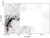 |
Fig. A.1. Brγ map obtained after continuum subtraction of the same area of Fig. 1. The colored triangles depict identified MYSs with a K magnitude brighter than 14.5. The size of each point is proportional to its magnitude. |
Appendix B: Simulations
We conducted a permutation test to assess the likelihood of randomly finding a group of seven stars classified as MYSs with a velocity dispersion as low as that of Can1. The statistical test we used was the difference in the values of the velocity dispersion between the members of Can1 and the remaining field stars classified as late type, considering only stars with Ks magnitudes brighter than Ks = 14.5. The observed difference in the velocity dispersion for the real data is |σμCan1 − σμlate| = 1.98 mas/yr (dashed line in Fig.B.1). We then randomly shuffled the velocities between all the stars and compared the differences in the velocity dispersions. This process was repeated 20,000 times, and the results are shown in Fig. B.1. Only about 0.4% of the 20,000 simulated MYS groups had a |σμMYS − σμlate| equal to or higher than the real data (blue histogram to the right of the dashed line in Fig. B.1), indicating that the observed association of stars that formed Can1 is highly unlikely to have occurred by chance.
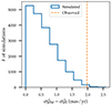 |
Fig. B.1. Velocity dispersion simulations. The blue histogram represent the difference in velocity dispersion between simulated populations of MYSs and late-type stars that where created by shuffling the velocities among the observed sample of stars. The dashed orange line represents the value between Can1 and the late-type stars. |
Appendix C: Results
In Fig. C.1, we depict the members of the comoving group found by Martínez-Arranz et al. (2022) in blue and Can1 in orange. We mark in green the members of Can1 with a counterpart in the comoving group (Mar23). Can1 appears to be part of a larger comoving group whose members extend beyond the KMOS field we analyzed here. Further KMOS data will be acquired in an adjacent area (dashed gray square in the image) to confirm this observation.
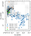 |
Fig. C.1. Comoving group and MYSs on a the Brγ emission map. The orange triangle represents Can1 members. The blue points and circles represent the comoving group presented in Martínez-Arranz et al. (2024) (Mar23). The green triangles represent the elements in common between Can1 and Mar23. The dashed square outlines the region scheduled for observations using the KMOS instrument during ESO period P113. |
All Tables
All Figures
|
Fig. 1. KMOS field of view. The colored triangles depict identified MYSs with a K magnitude brighter than 14.5. The size of each point is proportional to its magnitude. The red square represents the area covered by a single IFU. The dashed black square represents the area covered by a single IFU after completing an observational sequence in the MOSAIC mode (16 pointings). The solid black box indicates the size of the fields into which we divided the image to be able to align them with the GC catalogs. |
| In the text | |
|
Fig. 2. Spectra of the MYSs. The MYSs are color-coded as in Figs. 1 and 3. In blue we show for comparison late-type spectra from stars in the field of approximately the same magnitude as the MYSs. |
| In the text | |
|
Fig. 3. KMOS object proper motions and CMD, and cluster simulation. The triangles represent Can1, and the blue circles represent the remaining objects in the field. Left: vector-point diagram. Middle: CMD. The vertical dashed line marks the color-cut we made to exclude foreground stars (H − Ks = 1.3). The horizontal dashed line marks the magnitude cut we made to exclude stars with low spectroscopic S/R (Ks = 14.5). Right: Spisea cluster simulation. The blue crosses represent members of a simulated cluster. The legend box displays the main features of the cluster. The shaded area represents the uncertainty in the position in the CMD for the members of the simulated cluster due to variations in extinction. |
| In the text | |
|
Fig. A.1. Brγ map obtained after continuum subtraction of the same area of Fig. 1. The colored triangles depict identified MYSs with a K magnitude brighter than 14.5. The size of each point is proportional to its magnitude. |
| In the text | |
|
Fig. B.1. Velocity dispersion simulations. The blue histogram represent the difference in velocity dispersion between simulated populations of MYSs and late-type stars that where created by shuffling the velocities among the observed sample of stars. The dashed orange line represents the value between Can1 and the late-type stars. |
| In the text | |
|
Fig. C.1. Comoving group and MYSs on a the Brγ emission map. The orange triangle represents Can1 members. The blue points and circles represent the comoving group presented in Martínez-Arranz et al. (2024) (Mar23). The green triangles represent the elements in common between Can1 and Mar23. The dashed square outlines the region scheduled for observations using the KMOS instrument during ESO period P113. |
| In the text | |
Current usage metrics show cumulative count of Article Views (full-text article views including HTML views, PDF and ePub downloads, according to the available data) and Abstracts Views on Vision4Press platform.
Data correspond to usage on the plateform after 2015. The current usage metrics is available 48-96 hours after online publication and is updated daily on week days.
Initial download of the metrics may take a while.