| Issue |
A&A
Volume 689, September 2024
|
|
|---|---|---|
| Article Number | A117 | |
| Number of page(s) | 12 | |
| Section | The Sun and the Heliosphere | |
| DOI | https://doi.org/10.1051/0004-6361/202449869 | |
| Published online | 06 September 2024 | |
The low-frequency power spectrum of slow solar wind turbulence
1
Department of Aerospace, Physics and Space Sciences, Florida Institute of Technology, Melbourne, FL 32901, USA
2
Johns Hopkins University Applied Physics Laboratory, Laurel, MD, USA
Received:
6
March
2024
Accepted:
11
June
2024
An important challenge in the accurate estimation of power spectra of plasma fluctuations in the solar wind at very low frequencies is that it requires extremely long signals, which will necessarily contain a mixture of qualitatively different solar wind streams, such as fast and slow wind streams, different magnetic polarities, or a mixture of compressible and incompressible fluctuations, along with other transient structures. This mixture of streams with qualitatively different properties unavoidably affects the structure of the power spectra by conflating all these different properties into a single power spectrum. In this work, we present a conditional statistical analysis that allows us to accurately estimate the power spectrum, at arbitrarily low frequencies, for “pure” slow solar wind streams, defined as those for which the solar wind speed is below 500 km s−1. The conditional analysis is based on the estimation of autocorrelation functions (ACF) of arbitrarily long but discontiguous signals, which result from excluding portions of the signal that do not satisfy the required properties. We use numerical simulations of magnetohydrodynamic (MHD) turbulence and magnetic field signals from the Wind spacecraft to test the estimator’s convergence to its true ensemble-averaged counterpart. Finally, we use this methodology on a fourteen-year-long Wind data interval to obtain the magnetic power spectrum of slow wind at extremely low frequencies. We show, for the first time, a full 1/f range in the slow wind, with a low-frequency spectral break below which the spectrum flattens and exhibits a well-defined peak at the solar rotation frequency.
Key words: Sun: magnetic fields / solar wind
© The Authors 2024
 Open Access article, published by EDP Sciences, under the terms of the Creative Commons Attribution License (https://creativecommons.org/licenses/by/4.0), which permits unrestricted use, distribution, and reproduction in any medium, provided the original work is properly cited.
This article is published in open access under the Subscribe to Open model. Subscribe to A&A to support open access publication.
1. Introduction
Early observations by Coleman (1968) revealed that the solar wind is turbulent and dominated by Alfvénic fluctuations, that is to say, highly correlated and non-compressible variations of velocity and magnetic fields with the characteristics of Alfvén waves, whose nonlinear dynamics are commonly described by incompressible magnetohydrodynamics (MHD). The power spectral densities (PSDs), also referred to as the power spectra, of these turbulent fluctuations in the solar wind exhibit multiple power laws over a broad range of frequencies (Kiyani et al. 2015), which are thought to be the result of an underlying energy spectrum established by a multi-scale nonlinear turbulence cascade (Verscharen et al. 2019). At very low frequencies, the PSD of fast solar wind streams exhibits a 1/f power law (Matthaeus & Goldstein 1986; Goldstein et al. 1995; Bruno et al. 2009) commonly identified as the turbulence energy-containing range. The origin of this 1/f range is still under debate; some authors suggest that it is produced at the Sun (Roberts 1989; Matthaeus & Goldstein 1986), whereas others suggest that it is formed in situ either by reflection-driven MHD turbulence (Velli et al. 1989; Verdini et al. 2012; Perez & Chandran 2013; Chandran & Perez 2019) or by the nonlinear evolution of the parametric decay instability (Chandran 2018; Davis et al. 2023; Huang et al. 2023). Matteini et al. (2018) connects the 1/f to the magnetic incompressibility of the turbulence, noting that this condition forces a saturation of the size of magnetic fluctuations on the largest spatial scales. The 1/f range is followed by the MHD inertial range with a Kolmogorov-like power-law scaling of f−5/3 (Russell 1972; Matthaeus & Goldstein 1986), akin to those characteristic of hydrodynamic turbulence (Frisch 1995). Although this dual power-law PSD at low frequencies was initially thought to be only found in the fast solar wind (Bruno & Carbone 2013), which is characterized by bulk speeds exceeding 600 km s−1 and high Alfvénicity (Belcher & Davis 1971), it has been partially observed recently in some Alfvénic (D’Amicis et al. 2019) and non-Alfvénic (Bruno 2019) slow wind streams.
An inherent difficulty in the estimation and interpretation of the PSD of solar wind observations at very low frequencies is that spectral analysis techniques require extremely long time signals, which unavoidably are bound to contain a mixture of various types of solar wind streams, such as slow and fast streams, mixed background magnetic field polarities, or a mixture of other transients (Bruno & Carbone 2013). This mixture of streams with qualitatively different properties necessarily affects the shape and structure of the PSD at very low frequencies when the PSD is estimated using standard spectral techniques for contiguous signals. Because the resulting PSD will contain spectral signatures of its different solar wind streams at all frequencies, its physical interpretation and its comparison with theoretical models may not be adequate. For instance, measurements of the PSD of plasma fluctuations in the solar wind are routinely compared to MHD turbulence models (Chen 2016) that describe how the energy is distributed in wavenumber space, which can be related to the PSD via Taylor’s hypothesis (Taylor 1938) or sweeping effects (Bourouaine & Perez 2018, 2019, 2020; Perez et al. 2021). Therefore, when the PSD is compared with a given turbulence model, we want the observed PSD to correspond to plasma fluctuations whose properties are as close as possible to those in the theoretical model being considered.
Traditional methods of finding suitable data intervals for a given study require finding near-contiguous periods of appropriate length with the desired parameter conditions. This length increases as one wishes to study lower frequencies, which in turn makes it more difficult to find suitable intervals. However, much longer intervals can be found by relaxing the need for contiguous data. This is done by conditioning the data, that is to say, removing portions of the signal that do not have the desired properties. This conditional analysis necessarily leads to discontiguous (or fragmented) signals. This approach was used by Bourouaine et al. (2020) to isolate switchbacks in Parker Solar Probe (PSP) data (Raouafi et al. 2023). The trade-off of this approach is that it requires a statistical analysis of fragmented signals with multiple gaps of varying sizes, for which spectral analysis based on the Fourier transform of contiguous signals is not adequate. For this reason, understanding how gaps created by conditioning affect the analysis is paramount for this methodology.
Data gaps, due to missing observations in an otherwise evenly spaced data sequence, have been investigated in solar wind turbulence signals (Kondrashov et al. 2010, 2014; Munteanu et al. 2016; Gallana et al. 2016). This analysis has been primarily motivated by undesired data gaps produced by spacecraft and instrument problems, such as missing points or other systematic causes of missing data. This problem is also found in many different fields: hydrodynamic turbulence (Maanen 1998), seismology (Baisch & Bokelmann 1999), stellar oscillations (Stahn & Gizon 2008), climatology (Moffat et al. 2007), and paleo-climatology (Rehfeld et al. 2011), where the size and distribution of the gaps determine how to best deal with them. A review of spectral analysis methods for non-uniformly sampled data can be found in Babu & Stoica (2010). A range of techniques for mitigating data gaps and non-uniformity are available: data gaps can be filled using interpolation or other advanced forms of reconstruction, the Lomb-Scargle method (Lomb 1976; Scargle 1982) fits non-uniformly sampled data to sinusoids using a least-squares method, and the CLEAN method improves estimates of periodograms by performing an iterative deconvolution in the frequency domain (Roberts et al. 1987). The effects of data gaps on various Fourier estimators have been thoroughly tested by Munteanu et al. (2016).
As opposed to previous works, we study the consistency (i.e., convergence properties) of a special type of the Blackman-Tukey (BT; Blackman & Tukey 1958) method designed to estimate the PSD of discontiguous (or fragmented) signals that arise from a conditional statistical analysis in which portions of arbitrarily long solar wind intervals are intentionally excluded from the analysis. This process results in a fragmented signal with multiple gaps of varying sizes, for which standard spectral analysis for contiguous signals may be inadequate. It is worth emphasizing that the focus of our analysis differs from previous works on gapped data in an important way, that is to say, previous works were mainly devoted to assessing and/or mitigating the effect of data gaps, using various techniques with different degrees of success (Gallana et al. 2016). More specifically, the focus of the analysis of signals with gaps until now has been on developing methodologies to recover the spectral properties of the full (“ungapped”) signal as accurately as possible from the same signal with gaps. In our approach, the gaps appear by choice from the conditional analysis, and a substantial increase in the length of the interval compensates for any potential adverse impacts that the gaps may have in the analysis.
Finally, we applied a conditional statistical analysis to estimate the PSD of slow wind using a 14-year-long Wind interval. This approach allowed us to obtain the PSD of “pure” slow solar wind streams at extremely low frequencies. This PSD captures, for the first time, the entirety of the 1/f range for slow wind, revealing a spectral break frequency at which the PSD flattens with superimposed peaks around the solar rotation frequency.
This paper is organized as follows. In Sect. 2, we present a brief summary of the basic elements of the spectral analysis used in this work and a description of the conditional estimation of the PSD. In Sect. 3, we test the validity of our conditional methodology for PSD estimation in MHD simulations and Wind data. In Sect. 4, we apply this methodology to a 14-year interval of Wind data to obtain a magnetic power spectrum of slow wind at extremely low frequencies. Sect. 5 summarizes our results.
2. Methodology
The PSD is fundamentally defined as the Fourier transform of the autocorrelation function (ACF) for stationary signals, which forms the basis of ACF-based PSD estimators like the BT method of spectral analysis (Blackman & Tukey 1958), whose mathematical and convergence properties have been well studied for decades (Ontes & Enochson 1972; Harris 1978; Nuttall 1981; Matthaeus & Goldstein 1982a). Here, we describe a specially crafted PSD estimator that extends the BT method to handle data with large amounts of data gaps. Similar correlation-based PSD estimators have been used before for gapped solar wind observations (Munteanu et al. 2016; Gallana et al. 2016; Bourouaine et al. 2020; Perez et al. 2021). However, these works were mainly focused on investigating the effect of undesired gaps associated with missing points on the estimation of the PSD and how to best mitigate them for a given solar wind signal of a fixed length. Furthermore, the consistency of PSD estimators for gapped signals (i.e., their convergence to the true ensemble-averaged PSD) has not been thoroughly documented with respect to data gaps.
In this section, we present the fundamental elements of PSD estimation theory for contiguous stationary signals that will help us introduce the relevant notation and context as we generalize this approach to the conditional estimation of the PSD for stationary signals; for more details, we refer the reader to any modern textbook in signal analysis, such as Alessio (2016).
2.1. PSD estimation theory
The PSD of a zero-average stationary random process x(t), which in principle represents any measured solar wind property, is formally defined as the Fourier transform of the ACF
where the ACF is defined as

E{⋯} denotes a statistical ensemble average (see the appendix), and τ is the time lag, defined as the time elapsed between the two measurements involved in the ACF. This definition is valid for signals whose ACFs are absolutely integrable (Alessio 2016), as is the case for stationary signals like those obtained from solar wind observations, where R(τ) is expected to drop to zero at sufficiently large τ. The most common approach to estimating the PSD of solar wind turbulence is based on the PSD of a finite-time signal PT(f), see, e.g., the appendix and Bourouaine & Chandran (2013), which is defined as
where XT(f) is the Fourier transform of the signal restricted to the interval t ∈ [0, T], that is,

The finite-length PSD can also be related to the ACF associated with the turbulent signal R(τ), defined in Equation (2) as
from where the Wiener-Khinchin theorem (WKT) follows in the limit (see Appendix A)
in which the full turbulence spectrum P(f) is recovered. The relationship between the finite-length PSD, PT(f), and the ACF established by Equation (5) forms the basis for correlation-based methods for estimating the PSD of stationary random processes. These methods seek an accurate estimate of the ACF from where the PSD follows via a suitable Fourier transform.
In practice, ensemble averages are estimated based on an ergodicity assumption, which states that the temporal average (over the variable t) equals the true statistical ensemble average E{⋯}. One important practical limitation of the ergodicity assumption in empirical signals, such as solar wind measurements, is that because they are necessarily of a finite length T and have finite resolution δt = 1/fs (where fs is the sampling rate), the convergence of estimated (or empirical) averages to their corresponding true ensemble value, such as in Equation (2), requires very long intervals and high sampling rates. Whether we estimate the PSD via Fourier-transform using Equation (3), or by estimating the ACF and using Equation (5), the empirical averages obtained from solar wind measurements are not guaranteed to converge to the true ensemble averages. Hence, all statistical averages obtained from empirical measurements represent approximations of their true values and, as such, are subject to statistical uncertainties beyond those associated with instrumental errors. The quality of an estimator from a signal with N measurements can be assessed in terms of the bias and the variance. The bias measures the difference between the estimated averages of a given quantity and its true statistical ensemble average, while the variance quantifies how much individual estimates spread around the ensemble average (see Appendix A). An estimator is said to be consistent if both bias and variance tend to zero when the number of measurements N becomes arbitrarily large.
The BT method for contiguous signals has three main steps: (1) estimation of the ACF from a finite signal; (2) application of a tapering window to the estimated ACF to reduce the variance of the resulting PSD at the cost of lower frequency resolution; and (3) computation of the discrete Fourier transform (DFT)1 of the windowed ACF, normally using a fast Fourier transform (FFT) algorithm.
For a discrete signal xn, where n = 0, 1, ⋯, N − 1, representing N consecutive measurements of the physical quantity x(t) with time resolution δt, the unbiased ACF estimator is defined as
where Nℓ is the number of available samples at time lag τℓ = ℓδt, and ℓ = 0, 1, ⋯, N − 1. The ACF for negative values of ℓ is obtained by symmetry of R(τ). When no gaps are present, Nℓ = N − |ℓ|. One main shortcoming of this estimator is that at high lags, Nℓ is very small, and so the estimation of the ACF becomes very poor. However, the use of this estimator in a discretized version of Equation (5) with T = TN = Nδt, leads to the following estimate of PT(f)
where  is the biased ACF estimator obtained by replacing Nℓ with N in Equation (7), which strongly reduces the weight of the estimated values of the ACF at high lags. In this equation, we chose to sample the estimated PSD on the discretized frequencies fk = kδf, δf = 1/(2Nδt), and k = −N + 1, ⋯, N. It then follows that the PSD estimated via Fourier-transform,
  , coincides with the DFT of the biased ACF estimator. The ACF-based estimator for the PSD defined in Equation (8) is known to be a bad estimator of the PSD in the sense that it is not consistent; specifically, its variance does not decrease with increasing N, as expected from a reliable (consistent) estimator. For this reason, the BT method adds a tapering window wM(τ) to artificially suppress the poorly estimated values of the ACF at a time TM that is much shorter than the length of the signal TN. As shown in Appendix A, this is equivalent to a smoothing of the PSD in Equation (8) through a moving average over a small window of size δf = 1/2Mδt around each frequency, resulting in a strong reduction of the variance (Alessio 2016).
2.2. PSD estimator for discontiguous signals
The estimator we investigate when gaps are present follows the same steps as the standard BT, with one important difference: the missing products are removed from the sum in Equation (7). This gapped ACF estimator can be more precisely defined if we assume that our measured signal xn can be represented as pnXn, where Xn is the theoretical ungapped signal, and pn is another random sequence that is zero when the measurement n is not available (gap) and unity when the measurement is available. In this case, the unbiased gapped ACF estimator can be written as (Gallana et al. 2016)
where
is the number of samples available at lag ℓ. In this work, we quantified the number of gaps in a signal using the total gap percentage (TGP), which is the ratio of the number of gaps to the total length of the signal:
For higher TGPs, the difference between Nℓ and N does become significant even at low lags. We find that it is necessary to use an unbiased ACF estimator under these conditions to obtain good estimates of the PSD.
Consistent with the BT method, we multiplied the estimated ACF,  , by a tapering window function wM(τℓ), where wM(τℓ) = 0 for |ℓ| ≥ M. While this limits the maximum lag of the ACF, which yields a decrease in frequency resolution, the variance of the PSD is greatly reduced. In this work, we only considered the Bartlett window wM(τℓ) = 1 − |ℓ|/M. Other types of windows, such as Hamming or Hanning, can be used but are beyond the scope of this paper. We want to emphasize that while, in general, the BT method leaves the choice of tapering window to the user, the Bartlett window coincides with the expression for PT(f) given in Equation (5).
The PSD estimator then follows by performing a DFT of the gapped ACF estimator tapered with a Bartlett window. We write the discretized version of Equation (5) as
where we introduce the discretized frequency fk = kδf, δf = 1/(2Mδt), and k = −M + 1, ⋯, M. In this expression, we have taken T = TM ≡ Mδt, as we describe in more detail in Appendix B. It is worth noting that the frequency resolution for this estimator is lower than the more traditional PSD obtained via the FFT of the full signal in the range [0, TN], where TN = Nδt, in which case the resolution is δf = 1/2Nδt. In the following section, we test the consistency of the estimator defined in Equation (12), that is, its convergence to the true ensemble average with decreasing statistical uncertainty as N is increased.
3. Conditional PSD tests for MHD simulations and solar wind observations
Whether discontiguous signals arise from missing data or conditioning, data gaps often come in clusters, a situation that is commonly associated with long-term equipment malfunction or with mixed streams where not all available data are deemed suitable for analysis. The ACF can still be estimated from some signals with these types of gaps, as points on either side of the gap could still be correlated with each other. We tested this type of gap configuration using the many-large-gaps (MLG) method. The correlation length or time of the signal without added gaps was initially measured. Then, clusters of gaps were generated, each with a length between 50% and 150% of the correlation length with uniform probability, until the desired TGP is reached. The spacing and exact location of each cluster was determined using a Dirichlet distribution. Given g clusters of gaps, we used the Dirichlet distribution to generate a random series, xi, of g + 1 values such that  . These values were scaled and rounded so that we end with a series of integers that sum to the length of the signal minus the total length of the cluster of gaps, which were interwoven with the previously generated clusters of gaps to create the gap signal pn. This method ensures that adjacent clusters of gaps do not overlap, although they are allowed to neighbor each other.
While large clusters of data gaps do occur, sometimes it is just a single point or a small cluster of points missing in an otherwise contiguous signal. For this type of gap, we used the uniformly distributed gaps (UDG) method, where for each point in the signal, a random number between 0 and 1 with uniform probability was generated. Those points whose random number is less than the specified TGP were removed, creating a new signal with data gaps. The TGP of the new signal is usually within 1% of the specified TGP and improves with the length of the signal.
In the following, we estimated the PSD for magnetic field signals with both types of gaps in simulated MHD turbulence (Sect. 3.1) and intervals of fast and slow wind from Wind (Sect. 3.2), to determine the effects that the distribution and size of data gaps have on the estimated ACF and corresponding PSD, for a fixed data size. Gaps were applied at 10%, 30%, and 50% TGPs for each test. Figure 1 shows sample signals with and without gaps from the simulated and Wind data. The advantage of these tests is that because the gaps are artificially introduced, we can compare the PSDs estimated for each TGP with the ungapped one. In Sect. 3.3, we investigate the consistency of the PSD estimator by establishing how its accuracy is increased, and its statistical variance is reduced with increasing N.
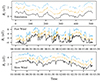 |
Fig. 1. Sample signals for each of the three datasets used in our analysis: simulated MHD turbulence, fast wind from Wind, and slow wind from Wind. The original signals are shown in black. The same signals with the UDG and MLG tests applied at a 30% TGP are shown in orange and light blue, respectively, and have been vertically offset for clarity. |
3.1. MHD simulations
We first studied the effects of data gaps on MHD turbulence by applying the two tests to magnetic field data from a steadily driven reduced MHD turbulence simulation (Perez et al. 2012). We took a single-time snapshot of the simulation. The simulation domain consists of a three-dimensional periodic box with L = 512 grid points along each direction. To keep in the statistics in the same order as the Wind case studies (see Section 3.2), we sampled 64 one-dimensional signals of length L. The signals each lie parallel to the edge of the box and each other, and are perpendicular to the mean field. Gaps were added to each signal, and the ACF of one of the perpendicular magnetic field components was calculated. The maximum lag was limited to L/2. The average of these ACFs was used to then calculate a single PSD. The results of both tests are shown in Figure 2.
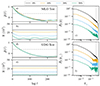 |
Fig. 2. Gaps test applied MHD turbulence simulations. Panels (a), (b), and (c) show the results of the MLG test. Panel (a) shows the normalized ACF; panel (b) shows the number of sampled pairs (in thousands) at each lag; and panel (c) shows the corresponding PSD of the ACF in panel (a). Panels (d)–(f) show the results of the UDG test and show the same quantities as panels (a)–(c), respectively. The black, orange, light blue and green lines are the tests run at 0%, 10%, 30%, and 50% TGPs, respectively. Units are grid points and grid wavenumbers. The PSDs have been artificially offset vertically. The horizontal lines in panels (a) and (d) mark the 1/e value. Vertical lines in panels (c) and (f) mark the high-frequency end of the inertial range in the simulation. |
Figure 2 plots the PSDs and their corresponding ACFs for both tests at TGP levels of 10%, 30%, and 50% each. The PSDs show good agreement in the low-frequency injection range and the mid-frequency inertial range when compared to the PSDs of the ungapped signal for both tests. However, in the high-frequency dissipation range, we see a significant increase in both bias and variance, and behavior changes with the gap distribution. For the MLG test, the spectra in this range follow a similar inertial range power law. The frequency at which bias and variance start to increase becomes smaller as the TGP increases. However, for the UDG test, the spectra level off and become flat past a certain cutoff frequency. The exact relation between the cutoff frequency and the TGP remains unknown. However, our results show that this frequency decreases with increasing TGP. This white-noise-like behavior is likely due to the random distribution of the gaps.
Each ACF estimate was normalized to its zero-lag value, denoted as  . Comparing the ACF estimates for gapped versus ungapped signals shows that the general shape of the ACF can be recovered for high TGPs for both tests, albeit with some superimposed noise. For the UDG test, this noise is short wavelength and small amplitude and appears like white noise, as further evidenced by the flattening of the corresponding PSD, whereas the MLG test appears to have longer wavelength fluctuations whose amplitude increases with the TGP.
It should be noted that we calculated the ACF by taking advantage of the periodic boundary condition so that there was no overhang of unmatched points typical of normal signal analysis. The resulting PSDs (before gaps are added) show much better agreement with the known power spectra of the simulation found via the FFT squared method. This also has the effect of ensuring that the statistics remain constant for all lags. When gaps are introduced, the statistics at any lag can fluctuate down from the base level seen at τ = 0 as gaps line up with data points (see Section 3.2 for a discussion on how gaps affect the statistics of nonperiodic signals, such as those in the solar wind).
3.2. Solar wind observations from Wind data
To see the effects of data gaps on real data, we applied the same tests on magnetic field measurements from Wind’s fluxgate magnetometer (Lepping et al. 1995). Wind is orbiting the L1 Lagrange point at a constant distance from the Sun in the ecliptic plane. The effects of the radial expansion on the magnitude of the magnetic field can, therefore, be ignored. We applied both tests to representative intervals of fast and slow wind. The data were re-sampled to a 24 s time resolution. For a closer analog to the simulated data, representing homogeneous turbulence, we filtered frequencies below the inertial range by subtracting the six-hour rolling average from the original signal. We calculated the trace of the PSD tensor for these case studies. The maximum lag calculated for the ACF was set to six hours, and we used the same TGPs as the simulation tests.
We analyzed a two-day period of fast solar wind starting at 00:00:00 on January 6, 2017. This period was chosen for its nearly homogeneous properties. The velocity remains between 675 and 750 km s−1 throughout the interval. The density is roughly constant and shows no major shocks or signs of other events. For our slow wind analysis, we chose a two-day period of slow solar wind starting at 00:00:00 on June 1, 2009. The velocity remains between 300 and 350 km s−1.
Figure 3 shows the probability distribution functions (PDFs) for the z-component of the magnetic field for the fast wind. Superimposed are the PDFs after we applied artificial gaps. In both cases, the resulting shape of the PDFs remain unchanged after applying gaps at all TGP levels. This shows that underlying statistics of the wind streams are not altered by applying gaps. However, this is not guaranteed in all cases and one should check the PDFs of all gapped data before analysis.
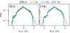 |
Fig. 3. PDF of the fast wind stream with artificial data gaps added. The data after the MLG method is applied are shown in the left panel, and the UDG method in the right panel. Both methods apply gaps at TGPs of 10%, 30%, and 50%. The dashed black lines show a centered Gaussian distribution with variance 2.2 nT for comparison. |
The results of the MLG and UDG tests are shown in Figure 4 for the fast wind and Figure 5 for the slow wind. In comparing the ACFs and PSDs from tests with gaps to the originals, we see many similarities to the simulation results in Figure 2. The ACF shows the same long and short fluctuations for the MLG and UDG tests, respectively. The spectral properties of the PSD can still be recovered except at the highest frequencies, f ≳ 3 × 10⁻³ Hz. Lower frequencies, however, appear largely unaffected.
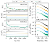 |
Fig. 4. MLG and UDG tests applied to fast wind interval from January 6–7, 2017. The panels have the same quantities as Figure 2. The statistics in panels (b) and (e) are shown in thousands. Note that the maximum lag shown is less than the six-hour maximum lag used to calculate the PSDs. |
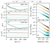 |
Fig. 5. MLG and UDG tests applied to the interval of slow wind from June 1–2, 2009. The panels have the same quantities and format as Figure 4. |
Due to the presence of data gaps, the statistics for the ACF, that is to say, the number of samples available at lag ℓ described in Equation (10), drop off faster than the linear relation Nℓ = N − |ℓ|, which is the expected relation for a signal without data gaps. This is most dramatic in the UDG test, where there is an immediate drop-off at ℓ = 1. Consider a single missing data point: when shifting the signal to calculate the ACF, this data gap will get lined up with its neighbor, which is a data point. In this way, many small data gaps will drastically cut into the total number of usable points at ℓ = 1. However, this immediately levels out and the statistics fall relatively linearly with some small amount of noise super-imposed. In contrast, large data gaps in the MLG test take a while to cover up a significant amount of data since, at low lags, they will mostly be lined up with themselves. Their statistics drop more slowly at low lags and fluctuate slowly as the different clusters of gaps pass each other.
3.3. Consistency of the estimator
Estimators of random signals are themselves random variables. The performance of an estimator is assessed via the bias and variance, which quantify the difference of the estimator from and spread around the true statistical value, respectively. For a random signal with N measurements, the estimator is said to be consistent if both bias and variance tend to zero in the limit N goes to infinity.
We applied a final set of tests to provide empirical evidence that the variance of the PSD estimator decreases as N increases. To vary N, we used the 24-day interval of non-Alfvénic slow wind starting on May 31, 2009, studied previously in Bruno et al. (2019). From this interval, subintervals of lengths 12, 6, and 3 days were created. The maximum lag was set to Mδt = 18 hours, which is 25% of the smallest subinterval. We first applied this test without any artificial gaps added. Then, to show that the presence of gaps does not negatively affect the consistency of the estimator, we repeated the process, adding gaps via the MLG method between 120 s and 2 hours at TGPs of 10%, 30%, and 50%. The results of all these tests are shown in Figure 6. From these results, it is clear that the variance of the PSD estimator decreases as we increase the size of the sub-intervals for all TGP tested. Moreover, it is demonstrated here that the increase in variance due to adding gaps is compensated by the increase in interval length. This can be seen by comparing the three-day interval at a 0% TGP to the 24-day interval at a 50% TGP, which has approximately the same variance.
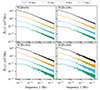 |
Fig. 6. Consistency test for our PSD estimator. In contrast to prior figures, the colors indicate the length of the subinterval. Gaps have been added using the MLG method with TGPs as indicated in the top left corner of each graph. The variance of each PSD clearly decreases as the length of the subinterval increases. All PSDs have been artificially offset vertically. |
4. The PSD of slow wind for very low frequencies
Based on the previous analysis, we can now use conditional statistics to isolate slow wind and construct a PSD with a frequency resolution corresponding to a year-long timescale, or about 1.6 × 10⁻⁸ Hz. This frequency resolution is far lower than what would be possible with traditional intervals while maintaining slow-wind conditions. In order to obtain a high accuracy and low variance PSD estimate, we used 14 years of Wind data from 2004 to 2017. The wind speed was smoothed using a two-hour rolling window. The data were then conditioned to only keep points with wind speed v < 500 km s−1. Before conditioning, this interval was missing 753 587 points, corresponding to a TGP of 4.1%; after conditioning, it was missing 18 410 385 points, resulting in a TGP of 27.3%.
The results of this conditional PSD analysis are shown in Figure 7. The inertial range is observed to follow a power law behavior with a spectral index α in the range near −5/3 as is normally expected for magnetic PSD at 1 AU (Podesta et al. 2007; Tessein et al. 2009; Podesta & Borovsky 2010; Boldyrev et al. 2011). Using a least-squares-fit in the range 2 × 10⁻⁴ Hz and 10−2 Hz gives a spectral index of −1.60. At low frequencies, we find that the PSD exhibits a full 1/f range spanning approximately one and a half decades, between 4 × 10⁻⁶ Hz and 10−4 Hz, corresponding to about 3 days and 3 hours, respectively. The least-squares fit for this frequency range gives a spectral index of −1.19.
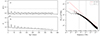 |
Fig. 7. Estimations of the PSD and ACF of the slow wind at 1 AU as found using conditioned Wind data. The panels have the same quantities and format as Figure 2. The dashed red lines the expected power laws for the inertial and 1/f ranges, shown for the sake of comparison. The vertical gray dashed lines show the approximate locations of the spectral breaks on both sides of the 1/f range. |
The spectral break separating the 1/f range from the inertial range at 10−4 Hz matches the one found by Bruno et al. (2019) for non-Alfvénic slow wind. This is in contrast to the location of the same break in the fast wind and Alfvénic slow wind, which is at ∼10−3 Hz (D’Amicis et al. 2019). It was noted in Bruno et al. (2019) that finding intervals of sufficient length, exceeding seven days, was a necessary but not sufficient condition for finding the 1/f range in the slow wind. They also observed that the magnitude of the normalized PSD was lower in intervals without the 1/f range, which may explain why our analysis shows such a robust 1/f range. Notably, with the long lags enabled by our methodology, it is possible to resolve, for the first time in the slow wind, a low-frequency spectral break in the 1/f range, approximately at 4 × 10⁻⁶ Hz.
Taking the upper-velocity limit of 500 km s−1, the slow wind takes about 3.4 days to travel one astronomical unit (1 au), corresponding to a frequency of 3.4 × 10⁻⁶ Hz which is the approximate location of the low-frequency spectral break in the 1/f range. This spectral break may be intrinsically tied to the travel time of the solar wind. Further tests are needed to quantify the radial evolution of the break in the slow wind or compare it to the location in the fast wind at 1 au, which should have a shorter travel time. At frequencies below this timescale, the PSD cannot represent the spatial structure of the turbulence. The PSD exhibits strong spikes corresponding to the solar rotation period (∼27 days). These are likely caused by the slow evolution of large-scale sources of the wind on the solar surface that last multiple rotations (Matthaeus & Goldstein 1986). The statistical data sample, or N in Figure 7, also shows a periodicity of the same 27 day frequency. This is likely due to the sources on the solar surface continuously producing slow wind over consecutive solar rotations. Using more conditions, it may be possible to find differences in this range for different types of solar wind streams.
Since this interval contains an entire solar cycle, calculating ACFs of this length requires sampling multiple streams. The pattern of slow wind streams creates a series of gaps similar to the MLG tests, which have little effect on the low-frequency part of the spectra. We can conclude that the entirety of the measured 1/f range is due to the properties of the slow wind itself. It is also worth noting that the interplanetary magnetic field has been shown to satisfy weak stationarity (i.e., convergence of the mean field and correlation to true ensemble averages) over several hundred of days (Matthaeus & Goldstein 1982b). While an analysis of this length will certainly sample different streams with differing properties, such as Alfvénic slow and the typical slow wind, we did not include conditions to discriminate between them. Over very long times, variations of the plasma parameters between different streams will be on shorter scales than the length of the data and are treated as fluctuations measured by the PSD. Rather, the mean values of the plasma parameters converge when averaged over a few solar rotation cycles and should be even more uniform than in the study by Matthaeus & Goldstein (1982b), whose analysis necessarily included mixed streams of fast and slow wind.
5. Conclusions
We presented a conditional spectral analysis to estimate the PSDs associated with solar wind streams that satisfy a set of prescribed, well-defined properties. This approach allowed us to obtain the PSD for “pure” slow wind streams at an extremely high resolution while maintaining the same underlying properties. The high frequency resolution is achieved because one can calculate the correlation up to extremely long time lags (up to and beyond one year) while averaging over the portions of the signal that match the desired conditions. We tested this PSD estimator in numerical simulations of MHD turbulence and Wind data to investigate (1) the effects of TGP and (2) its convergence to the true PSD when the sample (or interval) length is increased.
We tested two types of gap distributions: the MLG test, which removes clusters of consecutive points where each cluster’s size is on the order of the signals correlation length, and the UDG test, which removes random points from the signal with uniform probability. We applied these two tests to simulated data and to two intervals of Wind data. The results of all tests show that we can recover consistent estimates of both the ACF and PSD in the low to intermediate frequency range. We find that data gaps primarily affect the high-frequency range, whereas low frequencies were largely unaffected, indicating that conditioning data could be a very powerful tool for understanding the large-scale behavior of the solar wind. We show that our estimator is consistent by varying the interval length while maintaining a constant TGP. The results of these tests show that the variance of the PSD decreases as the length of the interval increases, which compensates the variance gained by the increasing TGP caused by conditioning.
These results are very similar to the small data gap test results for the Venus Express data by Munteanu et al. (2016), who found a similar overestimation in the high frequencies for all methods except the FFT with linear interpolation, which only slightly underestimated the spectrum in this range and could still recover the spectral slope. This supports their conclusion that linear interpolation may be the best way to handle small gaps in turbulent data.
By allowing fragmented or discontiguous data, one can find intervals of a single type much longer than what would be possible if one required near-contiguous data. Conditioning data isolates a single type of solar wind stream by removing points from an interval of mixed streams that do not have the associated properties of the desired stream type. While this does introduce new data gaps, the undesirable increase in PSD variance due to an increased TGP is offset by a comparable decrease in variance due to an increased interval length. Additionally, the increase in interval length allows one to probe frequencies lower than those that would normally be possible without mixing streams with substantially different properties.
The main result of this work is the application of this methodology to study the very low-frequency behavior of the slow solar wind at 1 au. Prior studies that have measured the solar wind in this frequency range necessarily used a mixture of fast and slow wind streams in their analysis (Matthaeus & Goldstein 1986) or limited the analysis to “pure” solar wind intervals of no longer than seven days (D’Amicis et al. 2019; Bruno 2019). The seven-day limit for solar wind intervals in the latter works limits the frequency resolution to 1.6 × 10⁻⁶ Hz, which can only capture a portion of the 1/f range. In contrast, our methodology allowed us to use 14 years of Wind data conditioned by the wind speed to determine the PSD of slow solar wind over six decades in frequency, from frequencies as low as ∼1.6 × 10⁻⁸ Hz (corresponding to year-long fluctuations) to frequencies of ∼2.1 × 10⁻² Hz (corresponding to fluctuation on a 1 min scale). This spectrum reveals, for the first time, a full 1/f range for slow wind with a low-frequency spectral break, below which the spectrum flattens and exhibits a well-defined peak at the solar rotation frequency, and a second spectral break frequency at the onset of the MHD inertial range. We suggest this methodology may be useful in investigating solar wind turbulence properties under different conditions.
Acknowledgments
MD, JC-Perez, JC-Palacios acknowledge support from NSF-SHINE grant AGS-1752827. SB and JC-Perez acknowledge support from NASA grant 80NSSC21K1768. MD, SB, and NER acknowledge support from the Parker Solar Probe project. Parker Solar Probe was designed, built, and is now operated by the Johns Hopkins Applied Physics Laboratory as part of NASA’s Living with a Star (LWS) program (contract NNN06AA01C).
References
- Alessio, S. M. 2016, Digital Signal Processing and Spectral Analysis for Scientists (Switzerland: Springer International Publishing) [CrossRef] [Google Scholar]
- Babu, P., & Stoica, P. 2010, Digital Signal Process., 20, 359 [NASA ADS] [CrossRef] [Google Scholar]
- Baisch, S., & Bokelmann, G. H. R. 1999, Comput. Geosci., 25, 739 [CrossRef] [Google Scholar]
- Belcher, J. W., & Davis, L. 1971, J. Geophys. Res., 76, 3534 [Google Scholar]
- Blackman, R. B., & Tukey, J. W. 1958, Bell Syst. Tech. J., 37, 185 [CrossRef] [Google Scholar]
- Boldyrev, S., Perez, J. C., Borovsky, J. E., & Podesta, J. J. 2011, ApJ, 741, L19 [Google Scholar]
- Bourouaine, S., & Chandran, B. D. G. 2013, ApJ, 774, 96 [Google Scholar]
- Bourouaine, S., & Perez, J. C. 2018, ApJ, 858, L20 [Google Scholar]
- Bourouaine, S., & Perez, J. C. 2019, ApJ, 879, L16 [Google Scholar]
- Bourouaine, S., & Perez, J. C. 2020, ApJ, 893, L32 [Google Scholar]
- Bourouaine, S., Perez, J. C., Klein, K. G., et al. 2020, ApJ, 904, L30 [Google Scholar]
- Bruno, R. 2019, Earth Space Sci., 6, 656 [NASA ADS] [CrossRef] [Google Scholar]
- Bruno, R., & Carbone, V. 2013, Liv. Rev. Sol. Phys., 10, 2 [Google Scholar]
- Bruno, R., Carbone, V., Vörös, Z., et al. 2009, Earth Moon Planets, 104, 101 [NASA ADS] [CrossRef] [Google Scholar]
- Bruno, R., Telloni, D., Sorriso-Valvo, L., et al. 2019, A&A, 627, A96 [NASA ADS] [CrossRef] [EDP Sciences] [Google Scholar]
- Chandran, B. D. G. 2018, J. Plasma Phys., 84, 905840106 [Google Scholar]
- Chandran, B. D. G., & Perez, J. C. 2019, J. Plasma Phys., 85, 905850409 [NASA ADS] [CrossRef] [Google Scholar]
- Chen, C. H. K. 2016, J. Plasma Phys., 82, 535820602 [Google Scholar]
- Coleman, P. J. 1968, ApJ, 153, 371 [Google Scholar]
- D’Amicis, R., Matteini, L., & Bruno, R. 2019, MNRAS, 483, 4665 [NASA ADS] [Google Scholar]
- Davis, N., Chandran, B. D. G., Bowen, T. A., et al. 2023, ApJ, 950, 154 [NASA ADS] [CrossRef] [Google Scholar]
- Frisch, U. 1995, Turbulence: The Legacy of A. N. Kolmogorov (Cambridge: Cambridge University Press) [Google Scholar]
- Gallana, L., Fraternale, F., Iovieno, M., et al. 2016, J. Geophys. Res.: Space Phys., 121, 3905 [NASA ADS] [CrossRef] [Google Scholar]
- Goldstein, M. L., Roberts, D. A., & Matthaeus, W. H. 1995, ARA&A, 33, 283 [NASA ADS] [CrossRef] [Google Scholar]
- Harris, F. 1978, Proc. IEEE, 66, 51 [NASA ADS] [CrossRef] [Google Scholar]
- Huang, Z., Sioulas, N., Shi, C., et al. 2023, ApJ, 950, L8 [NASA ADS] [CrossRef] [Google Scholar]
- Kiyani, K. H., Osman, K. T., & Chapman, S. C. 2015, Philos. Trans. R. Soc. A: Math. Phys. Eng. Sci., 373, 20140155 [CrossRef] [Google Scholar]
- Kondrashov, D., Shprits, Y., & Ghil, M. 2010, Geophys. Res. Lett., 37, L15101 [NASA ADS] [CrossRef] [Google Scholar]
- Kondrashov, D., Denton, R., Shprits, Y. Y., & Singer, H. J. 2014, Geophys. Res. Lett., 41, 2702 [NASA ADS] [CrossRef] [Google Scholar]
- Lepping, R. P., Acũna, M. H., Burlaga, L. F., et al. 1995, Space Sci. Rev., 71, 207 [Google Scholar]
- Lomb, N. R. 1976, Astrophys. Space Sci., 39, 447 [Google Scholar]
- Maanen, H. R. E. V., & Oldenziel, A., 1998, Meas. Sci. Technol., 9, 458 [NASA ADS] [CrossRef] [Google Scholar]
- Matteini, L., Stansby, D., Horbury, T. S., & Chen, C. H. K. 2018, ApJ, 869, L32 [Google Scholar]
- Matthaeus, W. H., & Goldstein, M. L. 1982a, J. Geophys. Res., 87, 6011 [Google Scholar]
- Matthaeus, W. H., & Goldstein, M. L. 1982b, J. Geophys. Res.: Space Phys., 87, 10347 [NASA ADS] [CrossRef] [Google Scholar]
- Matthaeus, W. H., & Goldstein, M. L. 1986, Phys. Rev. Lett., 57, 495 [Google Scholar]
- Moffat, A. M., Papale, D., Reichstein, M., et al. 2007, Agric. Forest Meteorol., 147, 209 [CrossRef] [Google Scholar]
- Munteanu, C., Negrea, C., Echim, M., & Mursula, K. 2016, Ann. Geophys., 34, 437 [CrossRef] [Google Scholar]
- Nuttall, A. 1981, IEEE Trans. Acoust. Speech Signal Process., 29, 84 [NASA ADS] [CrossRef] [Google Scholar]
- Ontes, R. K., & Enochson, L. 1972, Digital Time Series Analysis (New York: John Wiley& Sons) [Google Scholar]
- Perez, J. C., & Chandran, B. D. G. 2013, ApJ, 776, 124 [Google Scholar]
- Perez, J. C., Mason, J., Boldyrev, S., & Cattaneo, F. 2012, Phys. Rev. X, 2, 041005 [Google Scholar]
- Perez, J. C., Bourouaine, S., Chen, C. H. K., & Raouafi, N. E. 2021, A&A, 650, A22 [EDP Sciences] [Google Scholar]
- Podesta, J. J., & Borovsky, J. E. 2010, Phys. Plasmas, 17, 112905 [Google Scholar]
- Podesta, J. J., Roberts, D. A., & Goldstein, M. L. 2007, ApJ, 664, 543 [NASA ADS] [CrossRef] [Google Scholar]
- Raouafi, N. E., Matteini, L., Squire, J., et al. 2023, Space Sci. Rev., 219, 8 [NASA ADS] [CrossRef] [Google Scholar]
- Rehfeld, K., Marwan, N., Heitzig, J., & Kurths, J. 2011, Nonlinear Process. Geophys., 18, 389 [CrossRef] [Google Scholar]
- Roberts, D. A. 1989, J. Geophys. Res., 94, 6899 [NASA ADS] [CrossRef] [Google Scholar]
- Roberts, D. H., Lehar, J., & Dreher, J. W. 1987, AJ, 93, 968 [Google Scholar]
- Russell, C. T. 1972, Solar Wind (Washington: Scientific and Technical Information Office) [Google Scholar]
- Scargle, J. D. 1982, ApJ, 263, 835 [Google Scholar]
- Stahn, T., & Gizon, L. 2008, Sol. Phys., 251, 31 [NASA ADS] [CrossRef] [Google Scholar]
- Taylor, G. I. 1938, Proc. R. Soc. London Ser. A, 164, 476 [Google Scholar]
- Tessein, J. A., Smith, C. W., MacBride, B. T., et al. 2009, ApJ, 692, 684 [NASA ADS] [CrossRef] [Google Scholar]
- Velli, M., Grappin, R., & Mangeney, A. 1989, Phys. Rev. Lett., 63, 1807 [Google Scholar]
- Verdini, A., Grappin, R., Pinto, R., & Velli, M. 2012, ApJ, 750, L33 [Google Scholar]
- Verscharen, D., Klein, K. G., & Maruca, B. A. 2019, Liv. Rev. Sol. Phys., 16, 5 [Google Scholar]
Appendix A: Condensed review of the correlation and spectral analysis
Truly stationary processes cannot be realized experimentally because they require an ensemble of infinitely long signals (in time or space) that in practical applications do not exist. Another practical limitation of the analysis of random processes from empirical data is that averages from a finite data sample require extremely long records in order to converge to the true ensemble averages. As we show in this appendix, correlation and spectral analysis of finite-length signals combined with the ergodicity assumption can be used to make meaningful comparisons between theory and experiments/observations of stationary processes (Alessio 2016).
A random process x(t) can be seen as an ensemble of 𝒩 systems, each of which is found in one possible realization xs(t) of the random function x(t), where s = 1, 2, …, 𝒩 labels all possible realizations. In this sense, for each s, one obtains a regular (deterministic) function of t corresponding to a concrete realization. For a fixed t, one instead obtains all possible random values s = 1, …, 𝒩 that the function can take for that value of t, whose statistical properties (such as sample space and probability distribution) need not be the same. In fact, the probability density function is in general different at each t. A random process is said to be stationary if the statistical properties of the random function x(t) are identical at each time, which means any ensemble average involving x(t) is independent of time t. In this work we will made a milder assumption of stationarity, which is to assume that the mean μ, and the ACF, defined as

respectively, are time independent. The symbol E{⋯} is used to represent exact ensemble averages over an infinite number of realizations:
Processes that satisfy the two conditions in (A.1) are called wide-sense stationary (WSS). We only considered WSS processes that have a zero mean, and when this is not the case, we redefined the process by subtracting the mean μ from each realization xs(t), in which case the ACF becomes

In solar wind observations the function x(t) can represent any measured plasma or field property, such as particle number density, or any component of velocity and/or magnetic field measurement. Ensemble realizations, which we sometimes call signals, are obtained simply by taking multiple time subintervals of certain length T, where T is typically chosen to be longer than the turbulence correlation scale, ranging from a few hours to a few days. The multi-scale nature of the solar wind is evident from the observed PSD of solar wind measurements, in the form of multiple power laws that are often associated with turbulence cascades and other nonlinear plasma processes. For this reason, an accurate estimation of the PSD of solar wind measurements is important for the interpretation of solar wind observations and comparison with theoretical models and numerical simulations.
The PSD of a WSS signal within the time interval [0, T] is formally defined as
where
is the Fourier transform of x(t) restricted to the range [0, T]. The PSD defined in Equation (A.4) is also a random function because XT(f) is the Fourier transform of the random function x(t), and therefore may fluctuate from realization to realization. The PSD of the WSS process must then be obtained as the ensemble average
By far the most common technique to calculate the PSD of solar wind observations largely relies on an estimation of Equation (A.6) using a finite statistical sample, namely, a finite number of realizations on an evenly spaced temporal grid with a finite number of samples. These techniques focus on the evaluation of the DFT via the FFT algorithm on individual signals (or realizations), which are then averaged over a finite number of realizations, 𝒩:
where E𝒩{⋯} is defined as in Equation (A.2) with finite 𝒩 (without the limit), and the caret accent is used to differentiate estimated quantities from exact ones. Aside from the limitations associated with the discretization of the Fourier transform, which we discuss later, another limitation of this approach is that because T is necessarily finite, each realization in general might not capture the entire WSS process, discarding those timescales that are longer than T. In this sense, the true PSD of the WSS can only be attained for sufficiently large T:
Furthermore, the convergence of the estimated PSD  to the true one PT(f) can be only ensured for sufficiently large statistics (large 𝒩), hence
Alternative approaches to obtaining estimates of the PSD PT(f) are based on the WKT, which states that the true PSD P(f) and the true ACF R(τ) are Fourier transform pairs, that is to say

While the proof of this theorem is widely available (Alessio 2016), we present a succinct demonstration of the WKT because it will be useful in the description of ACF-based methods for estimating the PSD. Starting from equations (A.5) and (A.6) we have
The double integral in the previous equation can be recast in terms of new variables τ ≡ t′−t and u = t′+t − T in a simpler form
where wT(τ) is the window function wT(τ) = 1 − |τ|/T in the range [− T, T] and zero elsewhere, and A is the region shown in Figure A.1. In a not-so-rigorous fashion, we can take the limit T → ∞ to obtain

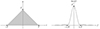 |
Fig. A.1. Integration region A after change of variables from t, t′ to τ, u. |
A more rigorous proof is to use the convolution theorem to write PT(f) in terms of the Fourier transform of R(τ), which we denote as S(f) and the Fourier transform of the window function wT(τ):
which as we show in Figure A.1, is well localized in a frequency range of length Δf = 2/T around zero. Furthermore, this function has the particular property that
From the convolution theorem it follows that
and therefore
from which we conclude that P(f) is the same as S(f), thereby proving the WKT.
An advantage from equation (A.20) is that the PSD PT(f) at each frequency f is actually a local average of the true PSD P(f) in a neighborhood of length Δf = 2/T around f. This averaging process over frequencies results in a smoothing of the true PSD P(f) over a frequency resolution Δf, essentially eliminating all processes that have a characteristic frequency below Δf, or equivalently, eliminating variations on timescales longer than T.
In summary, we have demonstrated that the PSD defined over a truncated time signal can be related to the Fourier transform of the exact correlation function via equation (A.16), or via the convolution of the true (ensemble averaged) PSD P(f) with the frequency-smoothing function ΔT(f) shown in Figure A.1. In the first case, this presents an alternative way to estimate PSDs from the Fourier transform of an estimate of the ACF instead of calculating the Fourier transform of individual signals. In the second case, we obtain the interpretation of PT(f) as a running average of the true PSD P(f) at each frequency with width Δf = 2/T, effectively removing all processes on a timescale longer than T.
Appendix B: PSD and ACF estimation from digital signals
In the following we assume that the WSS random process x(t) is sampled with a temporal resolution δt, resulting in a digital signal xn, where n = 0, 1, ⋯, N − 1, representing N consecutive measurements of a single realization of x(t) during a time interval T = Nδt. The PSD for this digital signal can be computed via the standard approach of evaluating the Fourier transform (A.5) on a discrete frequency grid fk = kδf with resolution δf = 1/Nδt, where k = 0, ±1, ±2, ⋯, ±N/2 (for even N), and calculating the integral on the discrete temporal grid tn = nδt
where XT, k is the DFT of the discrete sequence xn of length N
The PSD is then estimated by performing a simple average over 𝒩 realizations
The caret accent in  indicates that this is an estimated PSD and not the true PSD, which is obtained in the limit of an infinitely long signal (N → ∞) and an arbitrarily large number of realizations (𝒩 → ∞). An alternative approach is to estimate the ACF instead and obtain the PSD is via the relation (A.16). The simplest approach for evenly-spaced and ungapped signals of length N is to assume ergodicity, in which ensemble averages are replaced by temporal averages. This assumption is expected to hold if the signal is sufficiently long that it provides a representative sample of the full statistics of the random process.
For a WSS process represented by digital signals xn of length N, we evaluated the ACF, defined in equation (A.3), at time lags τℓ = ℓδt, with ℓ = 0, ±1, ±2, ⋯, ±(N − 1):
In this expression, the average is a true average over realizations of the WSS process. In practice, we often have a single realization, in which case the only way to perform statistics is to assume ergodicity to replace the average E{⋯} with a simple average over times tn:
where Nℓ is the maximum number of available samples at a given lag ℓ. The subindex u is used to indicate that this estimator is unbiased as we describe below. The major limitation of this estimator is that as the lag increases, the number of available samples for averaging decreases as Nℓ = N − |ℓ|, resulting in poor convergence to the true ACF at large values of |ℓ|. One characteristic of estimators in general is that they are themselves also random variables, because they are obtained as a function of a single random sample xn. This estimator is called unbiased because its ensemble average (over infinitely many realizations of the same process), coincides with the true expected average. This can be shown by performing the ensemble average of 

Using this unbiased estimator in equation (A.16) and calculating the integral on the discrete grid τℓ = ℓδt, we obtain an estimator of the PSD:

where
is the most commonly used ACF estimator. We note that this estimator is nearly identical to the unbiased one, except that Nℓ is replaced by the signal’s number of samples N, which as we can show it makes this estimate biased. The ensemble average of this estimator gives
This shows that, for low lags,  provides a good estimate of the true correlation R(τℓ), while at lags |ℓ| ≲ N, the convergence to the true ACF is poor. In the limit N → ∞ the estimate
  becomes unbiased. Equation (B.9) can be evaluated at the discrete frequencies fk = kδf, with δf = 1/2Nδt, to obtain
which is the DFT of the biased correlation.
The main disadvantage of these estimators for the PSD is that the poor estimation of the ACF at large lags |ℓ| ≲ N results in a large variance of the PSD at all frequency, resulting in a very noisy PSD estimator. A number of other methods are available in the literature that are devoted to decreasing the noise (or large variance) in the PSD associated with the lack of statistics of the ACF (biased or unbiased) at large lags. One widely used method for reducing the PSD variance from ACF-based estimators is the BT method (Blackman & Tukey 1958), which provides a smoother PSD estimator at the expense of decreased frequency resolution. The BT method is designed to minimize the effect of the poor statistics of the ACF at large lags by only considering its estimates up to a maximum lag ℓ = M ≪ N, where the ACF estimation is more accurate. The BT estimate of the PSD then corresponds to the true PSD of a signal within the interval [0, TM], where TM = Mδt ≪ T:
from where its estimated PSD follows
where fk = kδf and δf = 1/2Mδt. While the signal’s length is much larger, the BT estimate corresponds to the true PSD of a much shorter signal, with a lower resolution δf = 1/2Mδt. It is important to also keep in mind that we are using the same unbiased ACF as before, in which the averaging is performed over all the available samples at each lag Nℓ. As discussed in the previous section, it can be shown that the PSD  is a smoothed-out version of the estimate
  , obtained as the moving average over an interval of with δf around each frequency, which results in a substantial decrease in the variance.
All Figures
|
Fig. 1. Sample signals for each of the three datasets used in our analysis: simulated MHD turbulence, fast wind from Wind, and slow wind from Wind. The original signals are shown in black. The same signals with the UDG and MLG tests applied at a 30% TGP are shown in orange and light blue, respectively, and have been vertically offset for clarity. |
| In the text | |
|
Fig. 2. Gaps test applied MHD turbulence simulations. Panels (a), (b), and (c) show the results of the MLG test. Panel (a) shows the normalized ACF; panel (b) shows the number of sampled pairs (in thousands) at each lag; and panel (c) shows the corresponding PSD of the ACF in panel (a). Panels (d)–(f) show the results of the UDG test and show the same quantities as panels (a)–(c), respectively. The black, orange, light blue and green lines are the tests run at 0%, 10%, 30%, and 50% TGPs, respectively. Units are grid points and grid wavenumbers. The PSDs have been artificially offset vertically. The horizontal lines in panels (a) and (d) mark the 1/e value. Vertical lines in panels (c) and (f) mark the high-frequency end of the inertial range in the simulation. |
| In the text | |
|
Fig. 3. PDF of the fast wind stream with artificial data gaps added. The data after the MLG method is applied are shown in the left panel, and the UDG method in the right panel. Both methods apply gaps at TGPs of 10%, 30%, and 50%. The dashed black lines show a centered Gaussian distribution with variance 2.2 nT for comparison. |
| In the text | |
|
Fig. 4. MLG and UDG tests applied to fast wind interval from January 6–7, 2017. The panels have the same quantities as Figure 2. The statistics in panels (b) and (e) are shown in thousands. Note that the maximum lag shown is less than the six-hour maximum lag used to calculate the PSDs. |
| In the text | |
|
Fig. 5. MLG and UDG tests applied to the interval of slow wind from June 1–2, 2009. The panels have the same quantities and format as Figure 4. |
| In the text | |
|
Fig. 6. Consistency test for our PSD estimator. In contrast to prior figures, the colors indicate the length of the subinterval. Gaps have been added using the MLG method with TGPs as indicated in the top left corner of each graph. The variance of each PSD clearly decreases as the length of the subinterval increases. All PSDs have been artificially offset vertically. |
| In the text | |
|
Fig. 7. Estimations of the PSD and ACF of the slow wind at 1 AU as found using conditioned Wind data. The panels have the same quantities and format as Figure 2. The dashed red lines the expected power laws for the inertial and 1/f ranges, shown for the sake of comparison. The vertical gray dashed lines show the approximate locations of the spectral breaks on both sides of the 1/f range. |
| In the text | |
|
Fig. A.1. Integration region A after change of variables from t, t′ to τ, u. |
| In the text | |
Current usage metrics show cumulative count of Article Views (full-text article views including HTML views, PDF and ePub downloads, according to the available data) and Abstracts Views on Vision4Press platform.
Data correspond to usage on the plateform after 2015. The current usage metrics is available 48-96 hours after online publication and is updated daily on week days.
Initial download of the metrics may take a while.