| Issue |
A&A
Volume 689, September 2024
|
|
|---|---|---|
| Article Number | A308 | |
| Number of page(s) | 17 | |
| Section | Planets and planetary systems | |
| DOI | https://doi.org/10.1051/0004-6361/202449868 | |
| Published online | 24 September 2024 | |
Effect of the Earth’s declination variation on characteristics of Jovian decametric radio emissions
1
DIHPA, CGCE, Instituto Nacional de Pesquisas Espaciais (INPE),
São José dos Campos,
Brazil
e-mail: ezequiel.echer@inpe.br
2
LESIA, Observatoire de Paris, Université PSL, CNRS, Sorbonne Université, Université de Paris,
Meudon,
France
3
Observatoire de Radioastronomie de Nançay, Observatoire de Paris, Université PSL, CNRS, Univ. Orléans,
Nançay,
France
4
CCET, Departamento de Geofísica, Universidade Federal do Rio Grande do Norte (UFRN),
Natal,
Brazil
5
Aix Marseille Université, CNRS, CNES, LAM,
Marseille,
France
Received:
6
March
2024
Accepted:
17
July
2024
Context. The variation in the Jovicentric sub-latitude (declination, DE) of a radio observer of Jupiter has long been known to affect the observation of Jupiter’s decametric (DAM) radio emissions due to these emissions’ anisotropic nature (through cyclotron maser instability beaming cones centered on Jovian magnetic field lines). The effect of the DE variation, however, is still not clearly understood. For ground-based observations of Jupiter, the DE variation, from −4° to +4°, occurs concomitantly with the cyclic variation in the distance to Jupiter, R, and Jupiter’s elongation angle, γ, which also affect the emission observation. Those covariant effects must be removed, then, for an analysis of the pure effect of DE.
Aims. The aim of this study is to investigate the pure effect of the Earth’s DE variation on the maximum frequency, duration, average Io phase, and average longitude of Io-induced DAM emissions observed with the Nançay Decameter Array (NDA).
Methods. For this purpose, we selected from the NDA/Routine digital catalog Jovian DAM emissions with an intensity (distance-corrected) above or equal to 8.8 dB and a maximum frequency above or equal to 20 MHz (25 MHz) for southern (northern) emissions. Distinct maximum frequency thresholds were adopted because of the typical discrepancy in the emissions’ frequency due to the high amplitude anomaly in the Jovian magnetic field at Jupiter’s northern hemisphere. The selected emissions comprise a new “unbiased” catalog. After analyzing the tenuous variation in the characteristics of the unbiased set of Io-DAM emissions with DE, we compared them with those of matching Io-DAM simulations obtained with the Exoplanetary and Planetary Radio Emissions Simulator (ExPRES).
Results. From both the NDA data and the ExPRES simulations, it is observed that the pure DE effect on the Io-DAM emissions characteristics is minor, yet a clear proportionality of the maximum frequency and duration of the northern Io-DAM emissions with DE is noticed.
Conclusions. The northern Io-DAM emissions seem to be more strongly affected by the DE variation than the southern emissions. Additionally, ExPRES can predict Io-DAM emissions consistently, from which we conclude that the current understanding of emission generation and propagation is reasonable. This study may be extended for broader ranges of DE, such as Juno’s.
Key words: radiation mechanisms: non-thermal / methods: data analysis / catalogs / planets and satellites: individual: Jupiter / radio continuum: planetary systems
© The Authors 2024
 Open Access article, published by EDP Sciences, under the terms of the Creative Commons Attribution License (https://creativecommons.org/licenses/by/4.0), which permits unrestricted use, distribution, and reproduction in any medium, provided the original work is properly cited.
This article is published in open access under the Subscribe to Open model. Subscribe to A&A to support open access publication.
1 Introduction
The Jovian decametric (DAM) radio emissions observed between 10 and 40 MHz are long-known and extensively studied emissions whose origin is attributed to the cyclotron maser instability (CMI) (Wu & Lee 1979; Zarka 1998; Louarn et al. 2017; Collet et al. 2023), above the magnetic polar regions of Jupiter. They were first detected from the ground in 1955 by Burke & Franklin (1955) and gave the first indication that Jupiter has a strong magnetic field. These emissions result from the growth of radio waves through electron-wave resonance amplified at frequencies close to fce. The emissions are anisotropically beamed in thin hollow cones centered on the magnetic field lines (i.e., they are emitted in a specific direction, forming an angle, θ ± δθ/2, with the magnetic field lines with a thickness of δθ ~ 1° to 2°). Due to this anisotropic nature, the emissions’ observation depends on the position of the observer relative to the source. Therefore, the observation of Jovian DAM emissions from ground-based instruments is affected by the cyclic variation in the position of the Earth relative to Jupiter. Figure 1 represents the CMI beaming cone and the emission observation from a space probe.
It is long known that the variation in the Jovicentric declination (DE) of the Earth (i.e., the sub-Earth Jovicentric latitude), from −4° to +4°, affects the occurrence probability of the emissions, for instance, and most notably the width of the Io-Jupiter DAM emissions in diagrams of Jovicentric longitude versus the Io phase (Carr et al. 1970; Barrow 1981; Boudjada & Leblanc 1992; Leblanc et al. 1993; Garcia 1996). It is believed that this effect results from the CMI directivity combined with the complex Jovian magnetic field topology (asymmetric in the northern and southern hemispheres; Connerney et al. 2018), which makes emission visibility more or less favored as DE varies. However, this effect has still not been fully investigated or clearly understood. For instance, one intriguing behavior of the Jovian DAM emissions is that the majority of them are distributed in clusters around specific values of DE, such as −3.5°, −2°, 0°, 2°, and 3.5°, which suggests that the emissions are somehow better observed around every other 2° of DE (Jácome et al. 2023).
To study the statistical effect of DE on the observation of Jovian DAM emissions, we have taken advantage of the Jupiter observations collected since 1978 with different receivers connected to the Nançay Decameter Array (NDA) (Boischot et al. 1980; Lamy et al. 2017), which is the longest continuous database of Jovian DAM emissions. After a detailed analysis of this database, we have inferred that the clustered distribution of the emissions as a function of DE actually does not result from the variation in DE alone, but also from the variation in two other related parameters that affect the observation of the emissions simultaneously with DE: the Earth-Jupiter (E-J) distance (R) and Jupiter’s elongation angle (γ) (Garcia 1996; Jácome et al. 2023), which are sketched in Fig. 2. The variation in each of these variables of the E-J relative motion is covariant with the others, and therefore their effects on the emissions’ observation are combined. Here, γ ≥ 0° indicates that Jupiter leads the Sun (i.e., Jupiter rises and sets in the sky before the Sun) and γ < 0° that the planet trails the Sun (i.e., Jupiter rises and sets in the sky after the Sun).
The variation in R affects the emissions’ observation since their intensity varies in 1/R2. Thus, when R is greatest, only the most intense emissions can be detected. On the other hand, γ affects the emissions’ detectability by limiting the radio frequencies observed in good-enough conditions with ground-based instruments, since the cutoff frequency of the terrestrial ionosphere and the intensity of radio frequency interference (RFI) depend on the time of the day. When Jupiter is in opposition with the Sun (γ → ±180°), Jupiter is observed during the nighttime, when the cutoff frequency of the terrestrial ionosphere is minimum (around 10 MHz) and there is less RFI. When Jupiter is in conjunction with the Sun (γ → 0°), Jupiter is observed during daytime, when the ionospheric cutoff frequency is maximum (around 15 MHz) and the frequency range up to ~25 MHz is much more polluted by RFI, as is shown in the dynamic spectra of Fig. 3. Therefore, the observation of the emissions is favored by the shortest values of R and the opposition of Jupiter (γ → ±180°) which, for the NDA, always coincide with values of DE around −3.5°, −2°, 0°, 2°, and 3.5° (Jácome et al. 2023). Thus, in order to analyze the effect of DE variation alone on the observation of the Jovian DAM emissions with the NDA, it is necessary to remove the superimposed effects of γ and of R.
In this work, we present a selection of the Jovian DAM emissions from the NDA/Routine digital catalog (from 1990 to 2020) made in order to remove these superimposed effects. The emissions cataloged by Y. Leblanc from the NDA observations with other receivers over 1978–1990 (Leblanc et al. 1981, 1983, 1989, 1990, 1993; Lamy et al. 2023; Cecconi et al. 2023) are not considered here because of the lack of information on their intensity. We measured variations in the maximum frequency (Fmax), duration (Δt), average longitude (CML), and average phase of Io (ϕIo) versus DE for the unbiased sample. It was found that those variations are small. To check if this is compatible with our current understanding of the generation of Jovian DAM emissions, we compared the results from NDA observations with simulations of Jovian DAM emissions achieved with the Exoplanetary and Planetary Radio Emissions Simulator (ExPRES) (Louis et al. 2019). If ExPRES can consistently predict the emissions as they are recorded by the NDA and their variation with DE, the assumptions on which it is based (loss-cone-driven CMI and electron energy of a few keV) will be confirmed. Additionally, our understanding of the DE effect on the emissions’ visibility could be improved through the possibility of simulating emissions without the inherent limitations of ground-based observations; for instance, for comparison with observations with the Juno spacecraft (Bolton et al. 2017).
We restricted our analysis of the DE effect to the Io-induced (Io-DAM) emissions (Marques et al. 2017), induced by Alfvén waves generated in the electrodynamic interaction between Io and Jupiter’s rotating magnetic field, associated with well-defined small-scale sources near the footprints of Io’s magnetic flux tube. The other DAM components (either induced by Europa or Ganymede or not induced by moons) were disregarded because of the large extent of their source, which makes the analysis much more complex by adding free parameters. For Io-DAM emissions, we analyzed their variation within the total range of the Earth’s DE, relative to Jupiter, of ±4°.
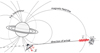 |
Fig. 1 Representation of a CMI beaming cone and the emission propagation, adapted from https://maser.lesia.obspm.fr/task-2-modeling-tools/expres/exoplanetary-and-planetary-radio.html?lang=en. |
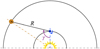 |
Fig. 2 Sketch (not to scale) of the Earth (in blue) and Jupiter (in orange) on their orbits, with the distance (R) and Jupiter’s elongation (γ). When γ = 0°, Jupiter is visible during daytime, and when γ = ±180°, Jupiter is visible during nighttime. |
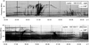 |
Fig. 3 Examples of dynamic spectra of Jupiter recorded by the NDA with its Routine receiver. The top panel illustrates the ionospheric and RFI conditions at night. The bottom panel illustrates those conditions during daytime. Vertical lines are calibration sequences. Jupiter’s decameter emission is structured in “arcs” in the t-f plane. The horizontal black lines are RFI. This figure is adapted from Lecacheux (2000). |
2 Data selection removing covariant effects
The emissions detected from 1990 to 2020 by the NDA/Routine are identified by eye from dynamic spectra-diagrams of intensity distributed in a time versus frequency (t-f) plane, and manually encircled by polygon selections within which emission properties are cataloged (see Appendix A of Marques et al. 2017). In the t-f planes, the Io-DAM emissions commonly form arc patterns that are referred to as vertex early arcs for the emissions from the dawn sector seen from Earth’s point of view (types B and D), and vertex late arcs for the emissions from the dusk sector (types A and C) (Boudouma et al. 2023).
In the NDA/Routine digital catalog, each emission has Fmax, minimum frequency (Fmin), and ephemeris data, such as the observer’s CML and the Galilean satellites’ phases and longitudes, listed at 1 minute resolution. The emission intensity corresponds to an estimate of the average intensity inside of the polygon area above the background intensity, in dB.
In order to analyze the pure effect of DE on the observation of emissions, we removed the superimposed effects of R and of γ by applying a selection of the emissions by their intensity and Fmax. The thresholds were determined by analyzing the variation in the Fmax of the emissions with γ and the intensity versus R (Fig. 4).
From the diagrams of Fig. 4, it can be understood that the Fmin of emissions observed by the NDA does not result from any physical elements involved in the origin of the emissions, but only from the cutoff frequency of the ionosphere, as is indicated by the modulation of the lower limit of the Fmin with the variation in γ. The lower limit is higher (~15 MHz) when Jupiter is seen in the day sky (γ → 0°) and lower (~10 MHz) when Jupiter is in the night sky (γ → ±180°). The Fmax, on the other hand, is not limited by the terrestrial ionosphere or RFI, but reflects the intensity of the magnetic field at the source of each emission. However, a modulation of the low values of Fmax with γ is also observed. This modulation is caused by the fact that the RFI hinders the distinction of the emissions: man-made RFI pollution reaches ~25 MHz during the day and is restricted to ≤10 − 15 MHz during the night. Only those emissions with Fmax higher than the RFI can be easily detected (by eye) on the dynamic spectra. Their low frequency extent is carefully searched by eye, then, through the RFI. The detection of an emission entirely drowned in RFI is much more difficult. This explains why the number of southern emissions diminishes so abruptly when Jupiter is observed during daytime (γ → 0°). With most of the southern emissions having maximum frequencies below 30 MHz, it is natural to infer that many of them are missed when the strong RFI is present up to 25 MHz.
The fact that the Fmax of the southern emissions is typically lower than that of the northern emissions – due to the higher intensity of the Jovian magnetic field in the northern hemisphere of Jupiter (Connerney et al. 2018, 2022) – explains why the defined thresholds are distinct for each hemisphere. If both thresholds were of 25 MHz, almost no southern emission would be selected. On the other hand, if both thresholds were of 20 MHz, the modulation observed in the Fmax low limit of the northern emissions would persist after the selection. Emissions with Fmax higher than or equal to those thresholds are detectable with the NDA, and distinguishable by eye regardless of γ.
The diagram of Fig. 4c shows the emissions’ intensity empirically corrected for R, in au. Those values of intensity are the cataloged intensities in dB above the background (galactic) corrected by R through the equation
![$\[I_{\text {cor }}=I_{\text {cat }}+10 \log (R),\]$](/articles/aa/full_html/2024/09/aa49868-24/aa49868-24-eq1.png) (1)
(1)
where Icat is the cataloged intensity, in dB, and Icor the corrected intensity, in dB. The analysis performed to obtain this correction equation is described in Appendix A. The correction was applied in order to estimate the original intensity of the emissions, and thus visualize the R effect on that parameter. Otherwise, no variation in the cataloged intensity in dB is observable as a function of R. This most likely results from observational limitations, such as the sensitivity of the NDA/Routine observations. Moreover, the emissions’ intensity as it is presented in the catalog is given as a function of the distribution of the observed intensity in the t-f plane and of the background. It does not express an instantaneous t-f measurement of the real intensity of the emissions.
After applying the correction in R on the emissions’ cataloged intensities (Fig. 4c), it became clear that, when R is large, only the most intense emissions can be detected with the NDA. We then set the intensity threshold to 8.8 dB, above which all the intensities are observable with the NDA regardless of the value of R (cf. Appendix A).
Figure 5 presents the distributions of Fmax and Fmin as a function of γ, and the distribution of the corrected intensities as a function of R for the Jovian emissions with Fmax and an intensity above the defined thresholds. From a total of 8997 emissions detected with the NDA/Routine from 1990 to 2020, 3094 emissions were found with Fmax higher than or equal to 25 MHz (20 MHz) for northern (southern) emissions and with a corrected intensity above 8.8 dB. From those, 1473 emissions are labeled in the catalog as Io-DAM A, B, C, or D, and 1140 emissions are labeled as not induced by Io. The remaining 4481 selected emissions are labeled as secondary Io-DAM emissions (Io-A’, Io-A”, or Io-B’) (Marques et al. 2017).
We next recalculated from this sub-catalog the emissions’ occurrence probability versus DE. Figure 6 shows the distribution of the occurrence probability of the selected emissions as a function of DE (in black). This occurrence probability was calculated from the ratio of the sum of Δt of the selected emissions found in each 0.25° bin of DE to the sum of Δt of the Jovian observations by the NDA/Routine found in the same 0.25° bin of DE. The occurrence probability distribution of all the emissions, from 1990 to 2020, without selection, is also shown for comparison. With the emission selection, we obtained a flatter probability distribution. Nevertheless, a smooth trend of increasing occurrence probability as DE increases is still present. From Fig. 6b, it is inferred that this trend is mostly due to the northern emissions. This higher dependence of northern emissions to DE could be due to the more complex topology of Jupiter’s magnetic field in the northern hemisphere.
In the NDA/Routine catalog, emissions of the same type are considered distinct emissions if the time gap between them is greater than 10 minutes. In practice, however, those distinct emissions might be different portions of a single arc that was not observed more integrally (see, for instance, the Io-B emissions detected on May 9, 1995, shown in Fig. 14 of Marques et al. 2017). In our analysis, when we had more than one Io-DAM emission of the same type in one observation, we considered them to be one single emission. Their Δt, then, became the time difference between the start of the first emission and the end of the last emission. Thus, 1350 main Io-DAM arcs were counted in our sub-catalog, instead of the previous 1473 main Io-DAM emissions. From these arcs, 550 are Io-A; 354 are Io-B; 283 are Io-C; and 163 are Io-D.
 |
Fig. 4 Distribution of the minimum and maximum frequencies (in MHz) and intensity (in dB above the background) of the Jovian DAM emissions on the NDA/Routine catalog as a function of γ (separately in the two hemispheres – a and b) and R (c), respectively. When γ → 0°, Jupiter is observed during daytime. Strong RFI and a high ionospheric cutoff frequency prevent detection below 15 to 20 MHz. When γ → ±180°, Jupiter is observed during nighttime. Weak RFI and a low ionospheric cutoff frequency allow detection down to ~10 MHz. The dashed red lines indicate the thresholds defined for the emission selection, at 20 MHz for the emissions from the Jovian southern hemisphere, at 25 MHz for the ones from the northern hemisphere, and at 8.8 dB for all the emissions. |
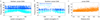 |
Fig. 5 Same as Fig. 4 but for the Jovian DAM emissions selected by Fmax and intensity from the NDA/Routine catalog. |
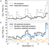 |
Fig. 6 Histograms of occurrence probability of the Jovian DAM emissions from the NDA/Routine catalog (1990–2020) as a function of DE. Panel a: for all the cataloged Jovian DAM emissions (dashed line) and for the selected emissions by Fmax and intensity (solid line). Panel b: the occurrence probability of the selected emission is also shown, separately, for the northern emissions (in blue) and the southern emissions (in orange). |
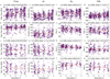 |
Fig. 7 Distributions of the Io-DAM main arcs’ (Io-A, Io-B, Io-C, and Io-D) Fmax, Δt, average ϕIo, and average CML as a function of DE. The red lines are linear fits to the data, with their slopes indicated on top of each plot. Between parentheses, there is the amount of arcs found for each type. |
3 Declination effect on the selected emissions
Figure 7 shows the distributions of the meaningful physical parameters that can be statistically studied versus DE from the above unbiased sub-catalog of Io-DAM arcs: Fmax, in MHz; Δt, in minutes; ϕIo, in degrees; and average CML, in degrees, as a function of the Jovicentric DE. The emissions’ Fmin is not physically sound because of variable obscuration by RFI. For each case, the distributions are greatly spread, in many cases not showing any clear dependence on DE, which is also indicated by the significantly small slopes of the linear fits (in red) of the data. Those slopes are indicated on top of each plot of Fig. 7. The dispersed distributions most probably result from the observational limitations and intrinsic emission variations.
From the linear fits of Fig. 7, we might infer that, overall, the DE variation effect on the Io-DAM emissions’ Fmax, Δt, ϕIo, and average CML is minimal. For Fmax (plots a, b, c, and d), the greatest absolute slope was obtained for the Io-A emissions, of 0.20 ± 0.05 MHz/degree, resulting in an average variation along the 8° range of DE of only 1.60 ± 0.40 MHz. For Δt (plots e, f, g, and h), the greatest absolute slope was obtained for the Io-B emissions, of 3.62 ± 0.61 min/degree, resulting in an average variation along the total DE range of 29.0 ± 8.48 minutes. For ϕIo (plots i, j, k, and l), the greatest absolute slope was obtained for the Io-D emissions, of 0.89 ± 0.25 degree/degree, resulting in an average variation of 7.12 ± 2.00° along the 8° total range of DE. Finally, for CML (plots m, n, o, and p), the greatest absolute slope was of −1.86 ± 1.39 degree/degree, obtained for the Io-D emissions. The average variation along the total DE range is of −14.9 ± 11.1°.
Both the Fmax and Δt distributions of the northern Io-DAM emissions show a smooth but clear increasing trend with DE. We see that the DE effect is stronger on the northern emissions than on the southern emissions, since no clear trend is observed for the southern emissions’ Fmax and Δt. Conversely, the distributions of the average ϕIo and average CML of the emissions show a stronger effect of DE on the Io-D emissions.
From the distributions of ϕIo it is observed that, as DE increases, the average ϕIo of the northern Io-DAM emissions (type A or type B) increases for the emissions from the dusk sector (A) and decreases for the emissions from the dawn sector (B). Conversely, for the southern Io-DAM emissions (type C or type D), the average ϕIo tends to decrease for the emissions from the dusk sector (C) and to increase for the emissions from the dawn sector (D). If we consider the complete arcs of Io-DAM emissions in the t-f planes, formed by the vertex early arc plus the vertex late arc, we may infer that the complete arcs generated in the northern hemisphere of Jupiter tend to cover a longer interval of ϕIo as DE increases, whereas those generated in the southern hemisphere tend to cover a shorter interval.
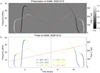 |
Fig. 8 Io-DAM arcs modeled by ExPRES for the December 13, 2020. The polarization of the arcs (a) and the respective values of the beaming cone aperture angle θ (b) are shown in t-f planes. The variation in the observer’s (at the Earth) ϕIo is shown in red in plot a, and the variation in ϕIo (PhIo) is indicated also in red in plot b. The dashed black line indicates the moment when ϕIo is 180°. For ϕIo < 180°, the emissions are labeled as Io-B or Io-D; and for ϕIo ≥ 180°, the emissions are labeled as Io-A or Io-C. |
4 Modeled Io-induced emissions
The observed variations versus DE are small. This may be partly due to the masking effect of the restricted observation window (~8h/day). In this context, the use of simulations of Jovian DAM emissions obtained with tools such as ExPRES (Louis et al. 2019, 2020) can be an interesting way to bypass the natural limitations of the ground-based observations and better understand the overall effects of the DE variation on the emission’s visibility. ExPRES has already been used several times to successfully model Jovian radio DAM emissions (see Hess et al. 2008a, 2010; Hess & Zarka 2011; Cecconi et al. 2012, 2021; Louis et al. 2017a,c; Hue et al. 2023). Our aim is to check if the observed variations versus DE can be understood via ExPRES simulations. The first step, though, was to check if these simulations can account for the statistical distribution of parameters Fmax, Δt, ϕIo, and CML (order 0), before searching for variations versus DE (order 1).
The simulations of Jovian DAM emissions analyzed in our study were developed with ExPRES for the main arcs of Io-DAM emissions (Io-A, Io-B, Io-C, and Io-D), generated by loss-cone-driven CMI – thus, θ is given as a function of frequency (Hess et al. 2008a), with electrons of 3 keV energy and a beaming cone δθ of 1° (Kaiser et al. 2000; Hess et al. 2008a; Louis et al. 2017c). No refraction was considered so that the modeled radio waves propagate in a straight line. The Jovian magnetic field was measured from the JRM09 model (Connerney et al. 2018) and the observer was fixed at the Earth. The lead angle between the active field line and the one connected to Io was estimated from the model proposed by Hess et al. (2011). The simulations are performed on a daily basis, from 1977 to 2024, and predict a broad range of values of θ, from below 40° to ~ 90°. The simulations were developed by Louis et al. (2023a).
One of the two main sources of uncertainty in ExPRES simulations of Io-DAM is the electron energy that is fixed in the simulations. It is found to vary within a 1–20 keV range as a function of time and altitude (Lamy et al. 2022). The other source of uncertainty is the estimation of the time of occurrence of the Io-DAM simulations. Io-DAM emissions can be estimated in a time window of ±2 h around the time of detection of the real emission (Louis et al. 2017b). This can in turn modify the shape of an Io-DAM arc, and therefore affect the comparison to the NDA data.
The products of those simulations are 24 hour long t-f plots with distributions of the modeled emissions’ θ and polarization, with supplementary data, such as the observer’s CML, DE, and R. The emissions’ dominant sense of polarization varies with the hemisphere of origin because it depends on the relative orientation of the wave vector, k, and the magnetic field, B (i.e., the k,B angle), at the emissions’ sources. Figure 8 shows the modeled Io-DAM emissions for December 13, 2020 as an example of the ExPRES simulations analyzed in this study. Figure 8a shows the polarization of the Io-DAM modeled emissions with negative (positive) values indicating polarization in the right-(left-)hand sense; thus, the emissions from the northern (southern) hemisphere of Jupiter. The CML of the observer is also presented, in red. Figure 8b shows the same modeled arcs but with the corresponding values of θ. The ϕIo is indicated in red.
The modeled arcs are in general longer than the Jovian DAM arcs observed with the NDA/Routine. The observed emissions typically consist of only the starting (vertex early) and ending (vertex late) portions of the arcs. Their central portion is not observed, possibly due to a flattening of the beaming emission cone and to refraction effects (Galopeau & Boudjada 2016; Lamy et al. 2022), and the observed portions are typically associated with beaming cone aperture angle, θ, varying between 70°−80° (Queinnec & Zarka 1998; Lamy et al. 2022). This real data constraint was applied to the simulations readings by setting minimum values for θ (θmin), varying from 65° to 81° with steps of 1°. No higher values were considered because, as θmin increases and reaches values above 80°, the modeled arcs become too short (i.e., reaching low Fmax), up to a stage at which the Fmax is below 10 MHz (i.e., no emission is identified in our reading). The simulations were read over the frequency interval of the observations: 10–40 MHz.
Lastly, another element that was taken into consideration in our reading of the ExPRES data was the possible uncertainty in the estimation of the simulations’ occurrence time. In order to test that uncertainty in the data, we considered the start and end times of the NDA observational window varying from −2 h to +2 h, with steps of 0.5 h. Each time shift, δt, was applied simultaneously to both the start and end times of the observations, so no variation in the time length of the observation was caused.
The first goal of this procedure is to determine the optimum values of δt and θmin by comparison with all selected observations, then check for a DE effect. Thus, the ExPRES data were read in a total of 153 different combinations of θmin and δt. In each of those cases, the Io-B/D and Io-A/C emissions were labeled from the portions of the modeled emissions occurring within the observational time window at ϕIo ranges of [0°, 180° [ and [180°, 360°[,respectively, so the typical observed ϕIo intervals of the Io-DAM were restricted in our reading by θmin and by δt alone.
Best θmin × δt sets for parameter and emission type.
5 Observed versus modeled emissions
In our comparison between the NDA data and the ExPRES data, we analyzed the same emission parameters presented in Fig. 7: Fmax, Δt, ϕIo, and CML of each Io-DAM arc. For each of the 153 combinations of θmin and δt considered in our analysis, we compared the Jovian DAM emissions from the NDA catalog with the ones obtained from the ExPRES simulations by calculating the mean absolute deviation (MAD) of each of the analyzed parameters between observations and their corresponding simulation. The MAD has the advantage of being less sensitive than the standard deviation to extreme values. It is defined as
![$\[M A D(X)=\frac{\sum\left|X_{\text {exp }}-X_{\text {nda }}\right|}{N_{\text {cases }}},\]$](/articles/aa/full_html/2024/09/aa49868-24/aa49868-24-eq2.png) (2)
(2)
where Xexp represents either Fmax, Δt, ϕIo, or the CML of one emission’s modeled arc; Xnda represents either of those parameters for the respective emission in the NDA data; and Ncases the number of days, in the years from 1990 to 2020, in which both modeled and real emissions of the same type were identified. In other words, Ncases is the total number of Jovian emissions of a specific type that were observed by the NDA and modeled by ExPRES – inside the observation window – in each set of δt versus θmin. The figures in Appendix B show the distribution of the MAD of each parameter of the emissions, calculated for each combination of δt versus θmin. In those distributions, the regions of minimum MAD vary by emission type and by parameter.
Overall, from the MAD values, Fmax is the parameter of the modeled arcs best matching that of the NDA arcs for all the main types of Io-DAM arcs, but especially for the southern ones, whose MAD minimum values are only around 2 MHz. The parameter of the modeled emissions worst matching that of the real arcs is Δt, with a minimum MAD value of 42.4 minutes, for the Io-B type.
Relative to the MAD values calculated for ϕIo and the CML of the arcs, the distributions in the δt versus θmin diagram are very similar, with the minimum MAD values for each emission type occurring around the same regions in the diagrams. The values of θmin and time shift associated with the minimum values of MAD of Fmax, Δt, ϕIo, and CML for each emission type were saved for further analysis of the best-fitting modeled emissions to the NDA emissions. They are shown in Table 1 with their mean and standard deviation for each emission type. Overall, the average θmin fluctuates around 72°. The average δt fluctuates around 0.44 h, but with a very significant dispersion.
To test the similarity between the simulations and the NDA data, we plotted Fmax, Δt, ϕIo, and CML of both simulations (only for the best θmin × δt sets) and their corresponding real emissions in Figs. 9–12, respectively. In those figures, the NDA data is presented in blue and the ExPRES data in red. The plots of the left column show the data in histograms, with the dashed lines indicating the respective average values. The corresponding θmin and δt are indicated on top of each of these plots. The plots in the central column are scatter plots showing the correlation between the modeled and real data. The green lines are linear fits to the data. The total number of emissions found in both simulations and in the NDA observations is indicated on top of each of those plots (count) with the correlation coefficient (corr) too. The plots of the right column show distributions of the emissions’ parameter (blue for the NDA data and red for the ExPRES data) as a function of DE, with linear fits to the data in similar colors. The slopes of the linear fits are indicated on top of the plots.
The NDA emissions shown in blue in the plots of Figs. 9–12 are a subset of those shown in Fig. 7. This occurs since, in the comparison with the modeled emissions, only the Io-DAM emissions that were detected in both the NDA data (selected by Fmax and intensity) and the simulations were considered. Modeled emissions might not be detected in our readings of ExPRES data for specific θmin × δt combinations. The absolute differences in the number of modeled emissions for each θmin × δt combination and the number of NDA emissions are shown in plot B.5 of Appendix B. In the best-case scenario (i.e., minimum count difference), the error found varies from ~0.3 to 8%.
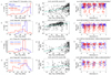 |
Fig. 9 Fmax of the arcs found both in the NDA catalog – after our emission selection – and in the ExPRES simulations, in the δt vs. θmin regions corresponding to the minimum MAD(Fmax) values. Left column: histograms of Fmax of the modeled Io-DAM emissions (in red) and of their corresponding emissions detected with the NDA (in blue). The dashed lines indicate the location of the mean Fmax value of each distribution. The emission type, the δt and θmin are indicated on top of the histograms. Mid column: scatter plots with the Fmax of the Io-DAM arcs observed with the NDA and the Fmax of the respective modeled arcs. The emission type, the correlation factor (corr), and the total number (count) of arcs found both in the real data (NDA arcs) and in the simulations (ExPRES) are indicated on top of the plots. Right column: distribution of Fmax of all the NDA Io-DAM arcs (in blue) and of the corresponding modeled arcs (ExPRES, in red) as a function of DE. The lines (in the respective colors) are linear fits to the data. The slopes of the linear fits are indicated on top of the plots (ExP for the modeled emissions – red; and NDA, for the NDA emissions – blue). |
5.1 Maximum frequency
Figure 9 shows the comparison of Fmax between the NDA emissions and their corresponding simulated ExPRES emissions. For the Io-A emissions, the values of θmin and δt associated with the minimum measured MAD(Fmax) are, respectively, 77° and −1 h. For the Io-B emissions, those values are 66° and 1.5 h; for the Io-C emissions, 70° and −0.5 h; and for the Io-D emissions, 69° and −0.5 h. In general, the emissions modeled at those conditions of θmin and δt present a broader range of Fmax, mostly toward lower frequencies, than that of the NDA emissions.
Relative to the number of emissions found in both the NDA catalog and the ExPRES simulations, 371 of the 550 selected Io-A arcs, 350 of the 354 selected Io-B arcs, 263 of the 283 selected Io-C arcs, and 158 of the 163 selected Io-D arcs were found in the simulations. The majority of the selected arcs, then, were somehow modeled and detected in our readings of the ExPRES data, and the distributions of Fmax of the respective NDA emissions as a function of DE (in blue, left column of Fig. 9) represent the distributions shown in Fig. 7 well, with slopes similar to those obtained before. The distributions of the modeled emissions (in red) as a function of DE, although with a larger Fmax range, present similar average Fmax and variation with DE, as is indicated by the proximity between the linear fits for modeled data and for real data. From the small slopes obtained, we confirm that the DE effect on the Jovian Io-DAM emissions’ Fmax seems pretty much null, as seen from Earth.
5.2 Duration
Figure 10 shows the comparison of Δt of the NDA emissions with that of their corresponding ExPRES emissions. For the Io-A emissions, the values of θmin and δt associated with the minimum value of MAD(Δt) are, respectively, 79° and 2 h; for the Io-B emissions, 75° and 0.5 h; for the Io-C emissions, 75° and 2 h; and for the Io-D emissions, 80° and 2 h. The emissions’ Δt was not well modeled. Both the histograms and the distributions of Δt of the ExPRES emissions as a function of DE do not match well those of the NDA emissions. This might be a consequence of the fact that Io-DAM emissions often display multiple arcs (see Figs. 3 and 14 of Marques et al. 2017 and Fig. 5 of Louis et al. 2019), while the modeled emissions are composed of one arc alone.
For the best sets of θmin and δt, according to the values of MAD(Δt), the total number of modeled emissions is 428 Io-A emissions, 312 Io-B emissions, 245 Io-C emissions, and only 88 Io-D emissions. In the scatter plots (plots e, f, and g of Fig. 10), we removed the ExPRES emissions with Δt longer than 140 minutes (for Io-A and Io-B) or 320 minutes (for Io-C) (~ 5% of the measurements), before computing their correlation with that of their corresponding NDA emissions. For the Io-D emissions, no removal procedure was applied.
5.3 Average lo phase
The plots of Fig. 11 show the comparison of average ϕIo of the NDA emissions with those of their corresponding ExPRES emissions. For the Io-A emissions, the values of θmin and δt associated with the minimum value of MAD(ϕIo) are, respectively, 65° and 0.5 h; for the Io-B emissions, 81° and −1 h; for the Io-C emissions, 65° and 1 h; and for the Io-D emissions, 68° and 0 h. In general, the average ϕIo of the emissions was well modeled for all four emission types considered.
For the best sets of θmin and δt, according to the values of MAD(ϕIo), the total number of modeled emissions is 504 Io-A emissions, 283 I-B emissions, 268 Io-C emissions, and 161 Io-D emissions. For all four emission types considered, both the histograms of the modeled emissions and of the NDA emissions, shown in the left column of Fig. 11, occur in the same ϕIo ranges and present similar distributions. This similarity between the real data and the modeled data is also indicated by the concurrent distributions of average ϕIo as a function of DE, and by the high correlation coefficients, greater than 0.5 (panels e, f, and g) except for the Io-D emissions, whose coefficient is equal to 0.26 (panel h). In the scatter plot relative to the Io-B emissions (panel f), we removed the ExPRES emissions with ϕIo smaller than ~92° or greater than ~107° (~4% of the measurements). This was applied to disregard the most incidental samples in the distribution and to better analyze the correlation (if any) between the remaining modeled emissions, comprising a narrower phase range, and their corresponding NDA emissions. For the other emission types, no removal was applied.
5.4 Average longitude
Finally, the plots of Fig. 12 show the comparison of average CML of the NDA emissions with those of their corresponding ExPRES emissions. For the Io-A emissions, the values of θmin and δt associated with the minimum value of MAD(CML) are, respectively, 66° and 1 h; for the Io-B emissions, 81° and 0 h; for the Io-C emissions, 65° and −0.5 h; and for the Io-D emissions, 67° and 0 h. In general, the CML of the emissions was well modeled for the emissions from the dawn side of Jupiter (from the observer’s point of view): the Io-B and Io-D emissions. For the Io-A and Io-C emissions, the average CML modeled is distributed in much broader ranges than those of the NDA emissions.
For the best sets of θmin and δt, according to the values of MAD(CML), the total number of modeled emissions is 505 Io-A emissions, 310 Io-B emissions, 269 Io-C emissions, and 161 Io-D emissions. For the Io-B and Io-D emissions, both the histograms of the modeled emissions and of the NDA emissions, shown in the left column of Fig. 12, occur essentially in the same CML range and present similar distributions (panels b and d). The similarity is also indicated by the high correlation coefficients, greater than 0.7 for the Io-B and Io-D emissions (panels f and h), and by the concurrent distributions of CML as a function of DE (panels j and l). For the Io-A and Io-C emissions, although the histograms of the modeled emissions do not match with those of the NDA emissions, the correlation coefficients are also high, of 0.68 for the Io-C emissions and of 0.4 for the Io-A emissions. In the scatter plot relative to the Io-B and the Io-C emissions (panels f and g), we removed the ExPRES emissions with average CML smaller than ~90° and ~210°, respectively, for a better analysis of the correlation between the remaining modeled emissions and their corresponding NDA emissions. Those remaining emissions correspond to 97 and 98% of the samples, respectively. The correlation coefficients were calculated for these emissions. For the other emission types, no removal was applied.
5.5 Emission distribution in the longitude versus Io phase diagram
As a last comparison between the simulations and the real Io-DAM emissions, we analyze the distribution of the emissions in the CML × ϕIo diagram, in Fig. 13. The diagrams a and b show the distributions of the Io-A and Io-B emissions, and of the Io-C and Io-D emissions, respectively, from the NDA/Routine catalog that were selected by Fmax and intensity. The other diagrams show the distributions of the ExPRES emissions modeled for each of the best θmin × δt sets (Table 1), according to the MAD values for each parameter analyzed and emission type.
We note that the ϕIo of the modeled emissions is highly consistent with that of the real emissions. In CML, on the other hand, the modeled emissions are much more spread than the real emissions. This might result from the fact that the CML varies in a much smaller period (~9.9 h) than that of the ϕIo (~42.4 h). Then, any small variation in the time of occurrence of the simulations, for instance, might be reflected in a significant variation in CML. Moreover, we might also infer that the variation in θmin affects the ϕIo range of the modeled emissions, their Δt, and, more smoothly, the CML interval of their occurrence. Either of those parameters is inversely proportional to θmin. One may compare, for instance, the Io-B modeled emissions in panels c, e and g of Fig. 13. In those cases the θmin was of 66°, 75°, and 81°, respectively. The δt may also play a role in those intervals.
Overall, the distributions in the CML versus ϕIo diagram of the modeled southern Io-DAM emissions are better correlated with the corresponding NDA emissions than the modeled northern emissions with their respective real emissions. This might result from the simpler magnetic field configuration in the southern hemisphere of Jupiter. For future analyses, simulations should be computed with more recent models of the Jovian magnetic field. Finally, we infer that the distributions of modeled emissions most similar to the real distribution were those for the Io-D emissions, both in CML and ϕIo.
6 Extending the analysis of the modeled declination effect
We have demonstrated that the real effect of the variation in the Earth’s DE on the average Fmax, Δt, ϕIo, and CML of the Jovian Io-DAM emissions observed with the NDA is indeed small over the ~8° amplitude range of DE. We have also demonstrated that ExPRES can consistently simulate Io-DAM emissions and fairly estimate the variation in those emissions’ average Fmax, ϕIo, and CML with DE. Thus, we may use ExPRES simulations to try to infer more precisely the expected effect of the variation in an observer’s DE relative to Jupiter on those characteristics of Jovian Io-DAM emissions.
Figure 14 shows modeled main Io-DAM emissions for November 14 and the 15, 2019. The arcs were simulated as if being detected by an observer with DE varying from −54° to +54°, with step of 36°, and with DE also at −4° and +4°, for comparison. The values of DE considered for this analysis were chosen, at first, to comprise evenly spaced values ranging from −90° to +90°, to simulate the effect of DE on observations of Jovian DAM emissions by the Juno spacecraft, for instance. However, no emission is observed at DE = ±90°. From the ExPRES simulations, it seems that no emission in the conditions considered can be detected by an observer located at DE ≥ ±65°.
In Fig. 14, the upper plot shows the modeled arcs originated in the northern hemisphere of Jupiter and the bottom plot shows the modeled arcs from the Jovian southern hemisphere. The colors indicate the observer’s DE. The arcs were developed for Io-DAM emissions generated by loss-cone-driven CMI with electrons at 3 keV of energy.
From Fig. 14a, it is noted that, as DE increases, the Fmax of the northern emissions also increases – at least up to DE = +18°, as well as the extent of the entire arc (i.e., the Io-(B+A) arc) on time and ϕIo. This agrees with what we have observed from the Io-A and Io-B emissions detected by the NDA from 1990 to 2020 (plots a, b, e, f, i, and j of Fig. 7). Moreover, the increase in Δt of the northern emissions with DE also explains the trend of increasing occurrence probability with DE, observed in Fig. 6.
For the southern emissions (Fig. 14b), on the other hand, as DE increases, the emissions’ Δt decreases, as does their Fmax. This behavior agrees only partially with what was observed for the Δt and Fmax of the Io-C and Io-D emissions detected with the NDA from 1990 to 2020, in plots c, d, g, and h of Fig. 7. Yet, although the linear fits to the distributions of Δt of the Io-C and of Fmax of the Io-D both present negative slopes, no clear effect of DE on those distributions is observed. Besides, the variation in the southern arcs’ complete extent (i.e., the Io-(D+C) arc) with increasing DE completely agrees with the variation in the average ϕIo of the Io-C and Io-D emissions (plots k and l of Figure 7), which suggests that the complete Io-(D+C) arc’s extent in ϕIo and Δt decreases with increasing DE.
Overall, we conclude from the simulations that the DE effect is minimum on the Fmax and Δt of the southern emissions at DE from −18° to +4°. For DE ≥ +18°, the DE effect is clearer on those characteristics of the southern Io-DAM emissions. The DE effect on the Fmax and Δt of the northern emissions is more expressive. In the Appendix C, we analyze these same modeled arcs but limiting them to the portions associated with θ ≥ 70°.
It is important to highlight that these simulations of arcs were made for one single period of 45 hours, taking into consideration, then, the exact same scenario – except for the observer’s latitude relative to Jupiter: the energy of the electrons, the Jovian magnetic field, the plasma density, the starting and ending locations of Io in the Jovian system, etc. By changing this scenario, a distinct relation between the emissions’ characteristics with DE might be observed. For a comparison with Juno observations, for instance, ExPRES simulations “à la carte” should be computed.
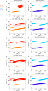 |
Fig. 13 Distributions of Io-DAM emissions in CML-ϕIo diagrams. Panels a and b: real Io-DAM emissions selected by Fmax and intensity from the NDA/Routine catalog. Panels c-j: modeled Io-DAM emissions for the best sets of θmin × δt, according to the MAD for emission type and parameter. |
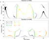 |
Fig. 14 Io-DAM emissions modeled with ExPRES for the days of November 14 and 15, 2019. The same emission is observed repeatedly for varying latitudes of the observer relative to Jupiter. |
7 Summary and conclusions
In this work, we present a way to study the pure effect of the variation in an observer’s DE relative to Jupiter on the observation of Jovian DAM emissions. For an observer located at Earth, such as the NDA, the pure DE effect can be studied after the removal of the superimposed effects of the variation in R and γ, which are coincident with the DE variation and which also affect the emission observation. We achieved this removal by setting thresholds for the emission’s Fmax, at 25 MHz for the northern emissions and 20 MHz for the southern ones, and for the emission intensity, at 8.8 dB, from which Jovian DAM emissions would be detected with the NDA/Routine regardless of R or γ. With those thresholds, we selected 1473 Io-DAM main emissions (Io-A, Io-B, Io-C, and Io-D emissions) from the NDA/Routine digital catalog to construct an unbiased sub-catalog for the analysis of the DE variation effect. This makes previous papers on the DE effect obsolete, such as Carr et al. (1970), Barrow (1981), Boudjada & Leblanc (1992), and Leblanc et al. (1993).
The DE effect was then analyzed for those emissions’ Fmax, Δt, ϕIo, and average CML. Overall, the DE effect seems to be minor, with the greatest absolute average variation of only 1.60 ± 0.40 MHz for Fmax along the total 8° range of the Earth’s DE; of 29.0 ± 8.48 minutes for Δt; of 7.12 ± 2.00° for ϕIo; and of 14.9 ± 11.1° for CML. However, those small variations might be a consequence of restrictions on the emission observation by ground-based observers, which cause the emissions to be observed only partially and can then hinder the DE effect. Additionally, the total variation in the Earth’s DE is also small, from −4° to +4°. Nevertheless, a smooth but clear trend of increasing Δt with DE is observed for the Io-A and Io-B emissions.
From the variation in the Io-DAM emissions’ average ϕIo, it is suggested that the total Io-B+Io-A arc’s extent in time and ϕIo tends to increase with increasing DE, whereas the total Io-D+Io-C arc’s extent decreases with DE. Sampling the CMI emission cone as DE varies is a fine remote diagnostic of the CMI operation at Jupiter that can validate or lead to improvements in the predicted beaming cone morphology.
We have also shown that ExPRES can consistently predict Io-DAM emissions with quite coincident Fmax, ϕIo and CML and, most importantly, the variation in those parameters with DE. This confirms not only that the observable effect of the DE variation is indeed small, but also that the current understanding of the generation (loss-cone-driven CMI) and propagation of the emissions is plausible. Moreover, the verified consistency of the ExPRES simulations also opens the possibility of studying the DE effect on the Jovian DAM emissions’ characteristics through simulations.
Overall, our analysis of the ExPRES data agrees with the range of the mid-aperture angle, θ, of the CMI beaming cone associated with the visible portions of the Io-DAM arcs, from 70° to 80° (Queinnec & Zarka 1998; Hess et al. 2008b; Louis et al. 2017c, 2023b; Lamy et al. 2022; Zheng et al. 2023). Regarding the possible uncertainty in the simulated emissions’ occurrence time relative to that of the real emission, no typical δt was detected.
We believe that the present paper closes the subject of ground-based study of the “DE effect” on Jupiter’s radio emissions, unless a database much longer than that of Marques et al. (2017) becomes available. At the same time, it lays the basis for a similar analysis based on Juno observations, which cover a much broader range of DE, from virtually −90° to +90°.
Data availability
The ExPRES simulations used in this work as well as other daily simulations of Jovian DAM emissions for other observers such as the Cassini, Voyager 1, Juno and Galileo spacecraft are available in CDF format at https://doi.org/10.25935/y0f3-9n63. The first published version of the digital catalog of the NDA/Routine, with data from 1990 to 2015, is available in multiple formats at https://doi.org/10.26093/cds/vizier.36040017. In this version, the emissions are distinguished by type and separated in two groups by satellite induction: Io-DAM or Non Io-DAM. The digitized version of the NDA catalog from 1978 to 1990 is available in JSON format at https://doi.org/10.25935/1FQM-FS07. The NDA/Routine data from 1990 (constantly updated) is available in CDF format at https://doi.org/10.25935/dv2f-x016. The daily dynamic spectra are also available.
Acknowledgements
This study was financed in part by the Coordenação de Aperfeiçoamento de Pessoal de Nível Superior – Brazil (CAPES) – Finance Code 001. E. Echer acknowledges financial support from the Brazilian agencies CNPq (PQ-301883/2019-0) and FAPESP (2018/21657-1). The Brazilian authors thank the Brazilian Ministry of Science, Technology and Innovation and the Brazilian Space Agency. The French co-authors acknowledge support from CNES and CNRS/INSU programs of planetology (PNP) and heliophysics (PNST).
Appendix A Analysis of the emissions’ intensity for correction in distance
In face of the fact that the cataloged intensity does not vary with R, in spite of what was expected, and since intensity ∝ 1/R2, we tried to estimate an approximation to the emissions’ original intensity. The correction should be Icor = Icat + 20 * log(R), where Icat is the cataloged intensity, in dB; R, the E-J distance, in au; and Icor, the corrected intensity, in dB. However, the limited sensitivity of the NDA, the averaging of the intensity above the background within the polygon and background fluctuations result in a weaker dependence of Icat on R.
Figure A.1a shows the histograms of observations (Nobs) of Jupiter (in black) and of Jovian DAM emissions (Nem), selected by Fmax, in each 0.1 au bin of R. Both from the NDA/Routine catalog. Figure A.1b shows the ratio Nem/Nobs, with a clear dependence on R. Considering that the decrease in Nem/Nobs with the increase in R is only due to the relation between the emission’s intensity and R, we intended to find a correction factor for the intensity and a threshold T so that the distribution Nem/Nobs as a function of R for emissions with Icor ≥ T is leveled.
Thus, we studied Nem parametrically for the emissions with Fmax ≥ 20 MHz (the southern ones) or Fmax ≥ 25 MHz (the northern ones). The intensity correction was applied through the equation
![$\[I_{ {cor }}=I_{ {cat }}+C * \log (R),\]$](/articles/aa/full_html/2024/09/aa49868-24/aa49868-24-eq3.png) (A.1)
(A.1)
where C is the correction factor, which varied from 5 to 20, step of 0.5. For each value of C, T varied from 0 to 20 dB (step of 0.1). We selected the (C,T) cases whose Nem(Icor) with Icor ≥ T was equivalent to at least 50% (i.e., 2810 emissions) of the total Nem selected by Fmax. For all those cases, linear fits were applied to the distributions of Nem/Nobs as a function of R. The linear fit’s slope and the standard deviation of each distribution around its fit were computed. We searched then for the cases with linear fit’s slope smaller than 0.01 and standard deviation smaller than 0.05. From the 11 (C,T) cases obtained, we chose the one with C = 10 and T = 8.8 dB.
Figure A.1c shows the histogram of Nem/Nobs in R for the emissions selected by Fmax and Icor, with C = 17.5 and T = 13.6 dB, for comparison with the equivalent histogram obtained with C = 10 and T = 8.8 dB, shown in panel d of Figure A.1. On top those plots, the slope of the linear fit (in red) to the histogram and the dispersion (sigma) around the fit are discriminated.
Appendix B Distributions of the mean absolute deviation in the time shift versus θmin plane
Figures B.1, B.2, B.3 and B.4 show the distribution of MAD of the emissions’ Fmax, Δt, average ϕIo, and average CML, respectively, calculated for each combination of δt versus θmin. The minimum and maximum MAD values calculated are indicated on top of the diagrams, and the dashed red lines delimit the region where the minimum value was found for each case. The values of θmin and δt associated with these regions of minimum MAD for each emission type analyzed (Io-A, Io-B, Io-C and Io-D) were the ones considered in the comparison between the modeled emission and the real emissions, in Sec. 5 of this article.
Only two distributions of MAD values are similar and present the minimum values around the same values of θmin and δt: the one for the emissions’ average ϕIo (Fig. B.3) and the one for the emissions’ average CML (Fig. B.4). The other two parameters (Fmax and Δt) present opposite distributions of MAD. For Fmax, the MAD values increase with increasing θmin because the modeled emissions became too short (both in frequency and in time) as θmin increased. For Δt, the greatest values of MAD accumulate around the smallest values of θmin because the modeled arcs became too long when θmin was smallest.
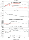 |
Fig. A.1 Representation of the parametric analysis of the distribution of Jovian DAM emissions (Nem) as a function of R. Panel a: Histograms of the observations (Nobs) of Jupiter (in black), and of Nem (in red) for emissions selected by Fmax from the NDA/Routine catalog. Panel b: Histogram of the ratio between the Nem and Nobs of panel a. Panel c: Histogram of the ratio Nem/Nobs for the emissions with intensity corrected with C = 17.5 above a threshold T = 13.6 dB. Panel d: Histogram of the ratio Nem/Nobs for the emissions with intensity corrected with C = 10 above a threshold T = 8.8 dB. N indicates the total number of emissions selected by Fmax with Icor ≥ T. The red lines are linear fits to the distributions. The linear fits’ slope is indicated on top of each diagram with the dispersion of the data around the fit (Sigma). |
Figure B.5 shows the distribution of the absolute difference between the number of modeled Io-DAM emissions and number of real Io-DAM arcs that were selected by intensity and Fmax. The count of the modeled emissions refers to the quantity of days in which one emission of a specific type was detected both in the real data (NDA catalog) and in the simulations (ExPRES data). The reference number of real Io-DAM arcs considered were those shown in Fig. 7.
From the minimum values shown on top of the diagrams of Fig. B.5, we note that the ExPRES modeled emissions of types Io-D and Io-B were the ones in most compatible quantity with that of the NDA emissions. For the Io-D emissions, there were 11 combinations of θmin and δt in which one only Io-D emission was observed in the catalog but not seen in the ExPRES simulations. Those cases are indicated in Fig. B.5d by the rectangles in salmon color. For the Io-B emissions, the one similar case is indicated by the dashed lines. Also, from the ratio of those minimum values at the top of the panels in Fig. B.5 to the numbers of observed NDA emissions (Fig. 7), we estimated a typical error in our comparisons with simulations: 43/550 (Io-A), 1/354 (Io-B), 12/283 (Io-C), and 1/163 (Io-D); that is, from 0.3% to 8%.
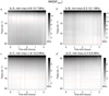 |
Fig. B.1 Distributions of MAD(Fmax) (in MHz) separated by emission type. The MAD(Fmax) was calculated between each real Io-DAM emission and its corresponding simulation, for each combination of δt and θmin considered in our analysis. The dashed red lines delimit the θmin and δt intervals associated with the minimum value of MAD(Fmax) for each emission type. |
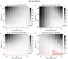 |
Fig. B.5 Distribution of the absolute differences between the count of Io-DAM emissions simulated by the ExPRES within the NDA observation windows and the count of real emissions observed by the NDA (after the selection by intensity and Fmax). The dashed lines indicate the regions of minimum difference. The salmon rectangles indicate the multiple regions where minimum difference in count was found for the Io-D emissions. |
Appendix C Limiting the modeled arcs by the associated θ
Figure C.1 shows Io-DAM emissions modeled by ExPRES for an observer with varying DE relative to Jupiter, from −54° to +54°, with steps of 36°, as well as the DE values of −4° and +4°, for comparison. Those modeled emissions are equal to those presented in Fig. 14, except for the fact that, in Fig. C.1, the portions presented are only the ones associated with θ ≥ 70°. By constraining the modeled arcs to θ ≥ 70°, it is noticed that, the once complete arcs become separated arcs – except at DE ≤ −18° for the northern emissions, and at DE = +54° for the southern emissions.
For the northern emissions (Fig. C.1a), the variation in θ from −18° to +18° affects differently the emissions’ occurrence time, Δt, and, more clearly, their Fmax, depending on the sector in Jupiter where the emissions are from. For the modeled Io-B (vertex early arc, originated at Jupiter’s dawn sector, at ϕIo smaller than 180°), the variation in Fmax becomes proportional to DE. For the Io-A emission (vertex late arc, originated at Jupiter’s dusk sector, at ϕIo from 180°), on the other hand, the Fmax is inversely proportional to DE. The Fmax of the southern emissions and the overall Δt of all the simulated emissions do not vary linearly with DE.
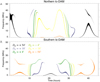 |
Fig. C.1 Io-DAM emissions modeled with ExPRES for the November 14 and 15, 2019, with θ ≥ 70°. The same emission is observed repeatedly for varying latitudes of the observer relative to Jupiter. |
References
- Barrow, C. H. 1981, A&A, 101, 142 [NASA ADS] [Google Scholar]
- Boischot, A., Rosolen, C., Aubier, M. G., et al. 1980, Icarus, 43, 399 [Google Scholar]
- Bolton, S. J., Lunine, J., Stevenson, D., et al. 2017, Space Sci. Rev., 213, 5 [CrossRef] [Google Scholar]
- Boudjada, M., & Leblanc, Y. 1992, Adv. Space Res., 12, 95 [NASA ADS] [CrossRef] [Google Scholar]
- Boudouma, A., Zarka, P., Magalhães, F. P., et al. 2023, in Planetary, Solar and Heliospheric Radio Emissions (PRE) IX, eds. C. K. Louis, C. M. Jackman, G. Fischer, A. H. Sulaiman, & P. Zucca (Dublin: Trinity College Dublin) [Google Scholar]
- Burke, B. F., & Franklin, K. L. 1955, J. Geophys. Res., 60, 213 [NASA ADS] [CrossRef] [Google Scholar]
- Carr, T. D., Smith, A. G., Donivan, F. F., & Register, H. I. 1970, Rad. Sci., 5, 495 [NASA ADS] [CrossRef] [Google Scholar]
- Cecconi, B., Hess, S., Hérique, A., et al. 2012, Planet. Space Sci., 61, 32 [Google Scholar]
- Cecconi, B., Louis, C. K., Crego, C. M., & Vallat, C. 2021, Planet. Space Sci., 209, 105344 [NASA ADS] [CrossRef] [Google Scholar]
- Cecconi, B., Debisshop, L., Lamy, L., & Genova, F. 2023, in Planetary, Solar and Heliospheric Radio Emissions (PRE) IX, eds. C. K. Louis, C. M. Jackman, G. Fischer, A. H. Sulaiman, & P. Zucca (Dublin: Trinity College Dublin) [Google Scholar]
- Collet, B., Lamy, L., Louis, C. K., et al. 2023, in Planetary, Solar and Heliospheric Radio Emissions (PRE) IX, eds. C. K. Louis, C. M. Jackman, G. Fischer, A. H. Sulaiman, & P. Zucca (Dublin: Trinity College Dublin) [Google Scholar]
- Connerney, J. E. P., Kotsiaros, S., Oliversen, R. J., et al. 2018, Geophys. Res. Lett., 45, 2590 [Google Scholar]
- Connerney, J. E. P., Timmins, S., Oliversen, R. J., et al. 2022, J. Geophys. Res. Planets, 127, e2021JE007055 [CrossRef] [Google Scholar]
- Galopeau, P. H. M., & Boudjada, M. Y. 2016, J. Geophys. Res. Space Phys., 121, 3120 [NASA ADS] [CrossRef] [Google Scholar]
- Garcia, L. N. 1996, PhD thesis, University of Florida, USA [Google Scholar]
- Hess, S. L. G., & Zarka, P. 2011, A&A, 531, A29 [NASA ADS] [CrossRef] [EDP Sciences] [Google Scholar]
- Hess, S., Cecconi, B., & Zarka, P. 2008a, Geophys. Res. Lett., 35, 13 [CrossRef] [Google Scholar]
- Hess, S., Mottez, F., Zarka, P., & Chust, T. 2008b, J. Geophys. Res. Space Phys., 113, 3260 [CrossRef] [Google Scholar]
- Hess, S. L. G., Pétin, A., Zarka, P., Bonfond, B., & Cecconi, B. 2010, Planet. Space Sci., 58, 1188 [Google Scholar]
- Hess, S. L. G., Bonfond, B., Zarka, P., & Grodent, D. 2011, J. Geophys. Res. Space Phys., 116, A5 [CrossRef] [Google Scholar]
- Hue, V., Gladstone, G. R., Louis, C. K., et al. 2023, J. Geophys. Res. Space Phys., 128, 5 [CrossRef] [Google Scholar]
- Jácome, H. R. P., Marques, M. S., Zarka, P., et al. 2023, in Planetary, Solar and Heliospheric Radio Emissions (PRE) IX, eds. C. K. Louis, C. M. Jackman, G. Fischer, A. H. Sulaiman, & P. Zucca (Dublin: Trinity College Dublin) [Google Scholar]
- Kaiser, M. L., Zarka, P., Kurth, W. S., Hospodarsky, G. B., & Gurnett, D. A. 2000, J. Geophys. Res. Space Phys., 105, 16053 [NASA ADS] [CrossRef] [Google Scholar]
- Lamy, L., Zarka, P., Cecconi, B., et al. 2017, in Planetary, Solar and Heliospheric Radio Emissions (PRE) VIII, eds. G. Fischer, G. Mann, M. Panchenko, & P. Zarka (Vienna: Austrian Academy of Sciences Press), 455 [Google Scholar]
- Lamy, L., Colomban, L., Zarka, P., et al. 2022, J. Geophys. Res. Space Phys., 127, e2021JA030160 [CrossRef] [Google Scholar]
- Lamy, L., Cecconi, B., Debisschop, L., et al. 2023, Icarus, 394, 115418 [NASA ADS] [CrossRef] [Google Scholar]
- Leblanc, Y., de La Noe, J., Genova, F., Gerbault, A., & Lecacheux, A. 1981, A&AS, 46, 135 [NASA ADS] [Google Scholar]
- Leblanc, Y., Gerbault, A., Rubio, M., & Genova, F. 1983, A&AS, 54, 135 [NASA ADS] [Google Scholar]
- Leblanc, Y., Gerbault, A., & Lecacheux, A. 1989, A&AS, 77, 425 [NASA ADS] [Google Scholar]
- Leblanc, Y., Gerbault, A., Lecacheux, A., & Boudjada, M. Y. 1990, A&AS, 86, 191 [NASA ADS] [Google Scholar]
- Leblanc, Y., Gerbault, A., Denis, L., & Lecacheux, A. 1993, A&AS, 98, 529 [NASA ADS] [Google Scholar]
- Lecacheux, A. 2000, in Radio Astronomy at Long Wavelengths, eds. R. G. Stone, K. W. Weiler, M. L. Goldstein, & J. Bougeret (Washington: American Geophysical Union), 1, 321 [CrossRef] [Google Scholar]
- Louarn, P., Allegrini, F., McComas, D. J., et al. 2017, Geophys. Res. Lett., 44, 4439 [CrossRef] [Google Scholar]
- Louis, C. K., Lamy, L., Zarka, P., Cecconi, B., & Hess, S. L. G. 2017a, J. Geophys. Res. Space Phys., 122, 9228 [CrossRef] [Google Scholar]
- Louis, C. K., Lamy, L., Zarka, P., et al. 2017b, in Planetary, Solar and Heliospheric Radio Emissions (PRE) VIII, eds. G. Fischer, G. Mann, M. Pachenko, & P. Zarka (Vienna: Austrian Academy of Sciences Press), 59 [Google Scholar]
- Louis, C. K., Lamy, L., Zarka, P., et al. 2017c, Geophys. Res. Lett., 44, 9225 [NASA ADS] [CrossRef] [Google Scholar]
- Louis, C. K., Hess, S. L. G., Cecconi, B., et al. 2019, A&A, 627, A30 [NASA ADS] [CrossRef] [EDP Sciences] [Google Scholar]
- Louis, C. K., Cecconi, B., & Loh, A. 2020, ExPRES Jovian Radio Emission Simulations Data Collection (Version 01)[Data set]. PADC [Google Scholar]
- Louis, C. K., Cecconi, B., & Loh, A. 2023a, ExPRES Jovian Radio Emission Simulations Data Collection (Version 11)[Data set]. PADC [Google Scholar]
- Louis, C. K., Louarn, P., Collet, B., et al. 2023b, J. Geophys. Res. Space Phys., 128, e2023JA031985 [NASA ADS] [CrossRef] [Google Scholar]
- Marques, M. S., Zarka, P., Echer, E., et al. 2017, A&A, 604, A17 [NASA ADS] [CrossRef] [EDP Sciences] [Google Scholar]
- Queinnec, J., & Zarka, P. 1998, J. Geophys. Res. Space Phys., 103, 26649 [NASA ADS] [CrossRef] [Google Scholar]
- Wu, C. S., & Lee, L. C. 1979, ApJ, 230, 621 [Google Scholar]
- Zarka, P. 1998, J. Geophys. Res. Planets, 103, 20159 [NASA ADS] [CrossRef] [Google Scholar]
- Zheng, R., Wang, Y., Li, X., Wang, C., & Jia, X. 2023, A&A, 673, A106 [NASA ADS] [CrossRef] [EDP Sciences] [Google Scholar]
All Tables
All Figures
|
Fig. 1 Representation of a CMI beaming cone and the emission propagation, adapted from https://maser.lesia.obspm.fr/task-2-modeling-tools/expres/exoplanetary-and-planetary-radio.html?lang=en. |
| In the text | |
|
Fig. 2 Sketch (not to scale) of the Earth (in blue) and Jupiter (in orange) on their orbits, with the distance (R) and Jupiter’s elongation (γ). When γ = 0°, Jupiter is visible during daytime, and when γ = ±180°, Jupiter is visible during nighttime. |
| In the text | |
|
Fig. 3 Examples of dynamic spectra of Jupiter recorded by the NDA with its Routine receiver. The top panel illustrates the ionospheric and RFI conditions at night. The bottom panel illustrates those conditions during daytime. Vertical lines are calibration sequences. Jupiter’s decameter emission is structured in “arcs” in the t-f plane. The horizontal black lines are RFI. This figure is adapted from Lecacheux (2000). |
| In the text | |
|
Fig. 4 Distribution of the minimum and maximum frequencies (in MHz) and intensity (in dB above the background) of the Jovian DAM emissions on the NDA/Routine catalog as a function of γ (separately in the two hemispheres – a and b) and R (c), respectively. When γ → 0°, Jupiter is observed during daytime. Strong RFI and a high ionospheric cutoff frequency prevent detection below 15 to 20 MHz. When γ → ±180°, Jupiter is observed during nighttime. Weak RFI and a low ionospheric cutoff frequency allow detection down to ~10 MHz. The dashed red lines indicate the thresholds defined for the emission selection, at 20 MHz for the emissions from the Jovian southern hemisphere, at 25 MHz for the ones from the northern hemisphere, and at 8.8 dB for all the emissions. |
| In the text | |
|
Fig. 5 Same as Fig. 4 but for the Jovian DAM emissions selected by Fmax and intensity from the NDA/Routine catalog. |
| In the text | |
|
Fig. 6 Histograms of occurrence probability of the Jovian DAM emissions from the NDA/Routine catalog (1990–2020) as a function of DE. Panel a: for all the cataloged Jovian DAM emissions (dashed line) and for the selected emissions by Fmax and intensity (solid line). Panel b: the occurrence probability of the selected emission is also shown, separately, for the northern emissions (in blue) and the southern emissions (in orange). |
| In the text | |
|
Fig. 7 Distributions of the Io-DAM main arcs’ (Io-A, Io-B, Io-C, and Io-D) Fmax, Δt, average ϕIo, and average CML as a function of DE. The red lines are linear fits to the data, with their slopes indicated on top of each plot. Between parentheses, there is the amount of arcs found for each type. |
| In the text | |
|
Fig. 8 Io-DAM arcs modeled by ExPRES for the December 13, 2020. The polarization of the arcs (a) and the respective values of the beaming cone aperture angle θ (b) are shown in t-f planes. The variation in the observer’s (at the Earth) ϕIo is shown in red in plot a, and the variation in ϕIo (PhIo) is indicated also in red in plot b. The dashed black line indicates the moment when ϕIo is 180°. For ϕIo < 180°, the emissions are labeled as Io-B or Io-D; and for ϕIo ≥ 180°, the emissions are labeled as Io-A or Io-C. |
| In the text | |
|
Fig. 9 Fmax of the arcs found both in the NDA catalog – after our emission selection – and in the ExPRES simulations, in the δt vs. θmin regions corresponding to the minimum MAD(Fmax) values. Left column: histograms of Fmax of the modeled Io-DAM emissions (in red) and of their corresponding emissions detected with the NDA (in blue). The dashed lines indicate the location of the mean Fmax value of each distribution. The emission type, the δt and θmin are indicated on top of the histograms. Mid column: scatter plots with the Fmax of the Io-DAM arcs observed with the NDA and the Fmax of the respective modeled arcs. The emission type, the correlation factor (corr), and the total number (count) of arcs found both in the real data (NDA arcs) and in the simulations (ExPRES) are indicated on top of the plots. Right column: distribution of Fmax of all the NDA Io-DAM arcs (in blue) and of the corresponding modeled arcs (ExPRES, in red) as a function of DE. The lines (in the respective colors) are linear fits to the data. The slopes of the linear fits are indicated on top of the plots (ExP for the modeled emissions – red; and NDA, for the NDA emissions – blue). |
| In the text | |
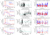 |
Fig. 10 Same as Fig. 9 but for Δt. |
| In the text | |
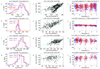 |
Fig. 11 Same as Fig. 9 but for ϕIo. |
| In the text | |
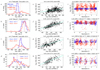 |
Fig. 12 Same as Fig. 9 but for CML. |
| In the text | |
|
Fig. 13 Distributions of Io-DAM emissions in CML-ϕIo diagrams. Panels a and b: real Io-DAM emissions selected by Fmax and intensity from the NDA/Routine catalog. Panels c-j: modeled Io-DAM emissions for the best sets of θmin × δt, according to the MAD for emission type and parameter. |
| In the text | |
|
Fig. 14 Io-DAM emissions modeled with ExPRES for the days of November 14 and 15, 2019. The same emission is observed repeatedly for varying latitudes of the observer relative to Jupiter. |
| In the text | |
|
Fig. A.1 Representation of the parametric analysis of the distribution of Jovian DAM emissions (Nem) as a function of R. Panel a: Histograms of the observations (Nobs) of Jupiter (in black), and of Nem (in red) for emissions selected by Fmax from the NDA/Routine catalog. Panel b: Histogram of the ratio between the Nem and Nobs of panel a. Panel c: Histogram of the ratio Nem/Nobs for the emissions with intensity corrected with C = 17.5 above a threshold T = 13.6 dB. Panel d: Histogram of the ratio Nem/Nobs for the emissions with intensity corrected with C = 10 above a threshold T = 8.8 dB. N indicates the total number of emissions selected by Fmax with Icor ≥ T. The red lines are linear fits to the distributions. The linear fits’ slope is indicated on top of each diagram with the dispersion of the data around the fit (Sigma). |
| In the text | |
|
Fig. B.1 Distributions of MAD(Fmax) (in MHz) separated by emission type. The MAD(Fmax) was calculated between each real Io-DAM emission and its corresponding simulation, for each combination of δt and θmin considered in our analysis. The dashed red lines delimit the θmin and δt intervals associated with the minimum value of MAD(Fmax) for each emission type. |
| In the text | |
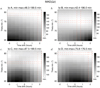 |
Fig. B.2 Same as Fig. B.1 but for Δt. |
| In the text | |
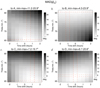 |
Fig. B.3 Same as Fig. B.1 but for ϕIo. |
| In the text | |
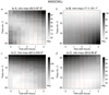 |
Fig. B.4 Same as Fig. B.1 but for CML. |
| In the text | |
|
Fig. B.5 Distribution of the absolute differences between the count of Io-DAM emissions simulated by the ExPRES within the NDA observation windows and the count of real emissions observed by the NDA (after the selection by intensity and Fmax). The dashed lines indicate the regions of minimum difference. The salmon rectangles indicate the multiple regions where minimum difference in count was found for the Io-D emissions. |
| In the text | |
|
Fig. C.1 Io-DAM emissions modeled with ExPRES for the November 14 and 15, 2019, with θ ≥ 70°. The same emission is observed repeatedly for varying latitudes of the observer relative to Jupiter. |
| In the text | |
Current usage metrics show cumulative count of Article Views (full-text article views including HTML views, PDF and ePub downloads, according to the available data) and Abstracts Views on Vision4Press platform.
Data correspond to usage on the plateform after 2015. The current usage metrics is available 48-96 hours after online publication and is updated daily on week days.
Initial download of the metrics may take a while.