| Issue |
A&A
Volume 689, September 2024
|
|
|---|---|---|
| Article Number | A4 | |
| Number of page(s) | 24 | |
| Section | Celestial mechanics and astrometry | |
| DOI | https://doi.org/10.1051/0004-6361/202449770 | |
| Published online | 03 September 2024 | |
A perturbative treatment of the Yarkovsky-driven drifts in the 2:1 mean motion resonance
1
School of Astronomy and Space Science, Nanjing University
Nanjing
210023,
PR China
e-mail: houxiyun@nju.edu.cn
2
Institute of Space Environment and Astrodynamics, Nanjing University,
Nanjing
210023,
PR China
3
Key Laboratory of Modern Astronomy and Astrophysics, Ministry of Education,
Nanjing
210023,
PR China
Received:
28
February
2024
Accepted:
5
July
2024
Aims. Our aim is to gain a qualitative understanding as well as to perform a quantitative analysis of the interplay between the Yarkovsky effect and the Jovian 2:1 mean motion resonance under the planar elliptic restricted three-body problem.
Methods. We adopted the semi-analytical perturbation method valid for arbitrary eccentricity to obtain the resonance structures inside the Jovian 2:1 resonance. We averaged the Yarkovsky force so it could be applied to the integrable approximations for the 2:1 resonance and the ν5 secular resonance. The rates of Yarkovsky-driven drifts in the action space were derived from the quasi-integrable approximations perturbed by the averaged Yarkovsky force. Pseudo-proper elements of test particles inside the 2:1 resonance were computed using N-body simulations incorporated with the Yarkovsky effect to verify the semi-analytical results.
Results. In the planar elliptic restricted model, we identified two main types of systematic drifts in the action space: (Type I) for orbits not trapped in the ν5 resonance, the footprints are parallel to the resonance curve of the stable center of the 2:1 resonance; (Type II) for orbits trapped in the ν5 resonance, the footprints are parallel to the resonance curve of the stable center of the ν5 resonance. Using the semi-analytical perturbation method, a vector field in the action space corresponding to the two types of systematic drifts was derived. The Type I drift with small eccentricities and small libration amplitudes of 2:1 resonance can be modeled by a harmonic oscillator with a slowly varying parameter, for which an analytical treatment using the adiabatic invariant theory was carried out.
Key words: celestial mechanics
© The Authors 2024
 Open Access article, published by EDP Sciences, under the terms of the Creative Commons Attribution License (https://creativecommons.org/licenses/by/4.0), which permits unrestricted use, distribution, and reproduction in any medium, provided the original work is properly cited.
This article is published in open access under the Subscribe to Open model. Subscribe to A&A to support open access publication.
1 Introduction
Resonance lock with dissipative effects occurs in various natural systems, such as in the dynamics of dust (Dermott et al. 1994), the satellites of major planets (Goldreich & Peale 1966), and exoplanets (Ferraz-Mello et al. 2003). We study in this paper the motions inside the Jovian 2:1 mean motion resonance (abbreviated as J2:1) with the Yarkovsky effect (Peterson 1976; Farinella et al. 1998), one of the dissipative effects that can cause secular orbital evolution of asteroids. Outside the resonance, the Yarkovsky mobility of the asteroid is mainly the secular drift of the semi-major axis (Bottke et al. 2001). We focus on the Yarkovsky-driven secular evolution of eccentricities of asteroids inside the J2:1. The stimulation of eccentricity of resonant asteroids is closely related to the depletion of the asteroids inside the Kirkwood gaps, among which the J2:1 is known as the Hecuba gap, and also closely related to the formation of near-Earth asteroids, whose size-frequency (Morbidelli & Vokrouhlický 2003), orbit (Granvik et al. 2018), and spin-state (La Spina et al. 2004; Liu et al. 2023) distributions may reflect the selection effects of the Yarkovsky effect.
Being a gap in the man belt with the largest width, the dynamics of the J2:1 resonance has been studied in detail (Morbidelli 2002; Nesvorný et al. 2002). The overlap of secondary resonances was found to produce a zone of chaotic motions at low to moderate eccentricity (Henrard & Lemaitre 1987), while the overlap of secular resonances was found to produce a large chaotic zone at a large eccentricity (Morbidelli & Moons 1993). For a large J2:1 libration amplitude and moderate inclination, a bridge connecting the two chaotic regions was also found to provide a route to escape with initially small eccentricity (Henrard et al. 1995). Nevertheless, there remains two quasi-stable islands away from any low-order resonances (Moons et al. 1998), inside which slow diffusive chaos was detected using numerical methods (Ferraz-Mello et al. 1998b) and explained by the resonance with the great inequality (Ferraz-Mello et al. 1998a).
The Hecuba gap is not completely depleted of asteroids (Roig et al. 2002): 374 resonant J2:1 asteroids with diameters 1~20 km were confirmed by Chrenko et al. (2015), of which around 230 are long-lived asteroids (with dynamical lifetime >0.7 Gyr) that reside in the quasi-stable islands mentioned above and in their vicinity and around 140 are shorted-lived asteroids (with a dynamical lifetime less than 0.7 Gyr) that reside in the chaotic regions. Brož et al. (2005) showed that due to the Yarkovsky drift of the semi-major axis, prograde rotators could be continuously pushed into the region occupied by the short-lived J2:1 population in order to maintain a quasi-steady state, but they can rarely enter the quasi-stable islands. The origin of the long-lived asteroids, whether primordial or through capture from main belts, still remains unsolved (Chrenko et al. 2015).
The stability of stable resonant J2:1 asteroids with respect to the Yarkovsky effect was investigated by Brož & Vokrouhlický (2008) using N-body simulation incorporated with the Yarkovsky effect. The systematic drift of eccentricity inside the resonance – a common characteristic for resonance lock with dissipative effects (Gomes 1995) – was found; the dynamical lifetime as a function of asteroid size for prograde rotators to gain critical eccentricity was obtained; and retrograde rotators were shown to be more likely to escape. The pioneering work by Brož et al. on the systematic drifts of eccentricity of resonant asteroids was mainly carried out in a numerical way. In this paper, we carry out a perturbative treatment using the semi-analytical approach suitable for the J2:1. In addition to the interaction between the Yarkovsky effect with the J2:1 resonance, we further consider its interaction with the v5 resonance inside the J2:1.
The contribution of this paper is twofold. The first part is a revisit of the resonance structures inside the J2:1 commensurability under the model of the planar elliptic restricted three-body problem (ERTBP). The first part has three components: the Schubart averaging of the planar ERTBP, Morbidelli’s elimination of the J2:1 harmonic (to be more specific, semi-analytical computation of the Arnold action variable of J2:1 resonance and the coordinate transform by the Henrard-Lemaitre formula), and the partial normalization of the secular Hamiltonian for the v5 resonance to the fourth order. For the first component, we complement the method developed in Moons (1994) by computing the transformation of variables between the complete system and the averaged system. The third component can be considered as a slight extension of the treatment of v5 resonance in Morbidelli & Moons (1993), where the integrable approximation of v5 resonance is obtained by a first-order perturbation theory.
The second contribution, which to our knowledge is original, is a perturbative treatment of the Yarkovsky-driven systematic drift in the action space of the J2:1 resonance. Under the model of planar ERTBP, we first identify two patterns of drift in the action space through numerical simulations: the first one (Type I) – already pointed out by Brož & Vokrouhlický (2008) – “walks” in the action space almost parallel to the curve of the stable resonance center of the J2:1 resonance; the second one (Type II) “walks” almost parallel to the curve of the stable resonance center of the v5 resonance. Our approach to analyze these two types of drift is close to that of Gomes (1995): the suitable form of the Yarkovsky effect averaged over the mean motions and the J2:1 resonance cycle is applied to the integrable approximations of the J2:1 resonance and the v5 resonance in order to obtain quasi-Hamiltonian systems from which a vector field of drift rates in the action space is derived.
For the Type I drift, the eccentricity increases (decreases) along the vector field for prograde (retrograde) asteroids. For prograde asteroids, we propose a fast algorithm to compute the Yarkovsky-driven excitation of the orbit eccentricity. Moreover, the Type I drift with small eccentricities and small libration amplitudes of the J2:1 resonance can be modeled by a harmonic oscillator with a slowly varying parameter. An analytical treatment of this simplified model using the classical adiabatic invariant theory was carried out and shows that for prograde (retrograde) asteroids, the J2:1 libration amplitude decreases (increases). We also find that the Yarkovsky-driven Type I drift for retrograde asteroids may serve as the mechanism to drive asteroids to the bridge identified by Henrard et al. (1995) that transfers them from the low-eccentricity chaotic regions caused by overlap of secondary resonances to the high-eccentricity chaotic regions caused by overlap of secular resonances. The N-body simulation results incorporated with the Yarkovsky effect confirm the existence of this evolutionary route for retrograde asteroids to escape the J2:1 resonance.
This paper is organized as follows. Section 2 presents the model and the method. Section 3 presents the results of the first part of the study on the resonance dynamics in the J2:1 resonance. Section 4 presents the results of the second part of the study on the Yarkovsky-driven drift in the action space. Section 5 discusses the Yarkovsky-driven escape of retrograde asteroids from the J2:1, and Sect. 6 concludes the study.
 |
Fig. 1 Schematic procedures of the perturbative treatments for the Yarkovsky-driven drifts in the J2:1 commensurability under the model of planar ERTBP. |
2 Model and method
The method adopted in this paper is schematically presented in Fig. 1. It consists of two chains corresponding to the two parts of studies mentioned in the introduction: (1) semi-analytical investigations on the dynamical structures in the J2:1 commen-surability in the canonical formalism. That is, a chain of three canonical transformations are applied to obtain a normal form of the Hamiltonian which can approximate well the secular dynamics inside the J2:1 commensurability; (2) averaging of the Yarkovsky force based on the aforementioned canonical transformations. The averaged Yarkovsky forces can be inserted into the canonical equations of the Hamiltonian system at different levels.
The first part starts with the Hamiltonian function HpERTBP of the planar elliptic restricted three-body problem (ERTBP). We include in the model a single-frequency precession of the Jupiter’s mean longitude of perihelion. Adopting a suitable canonical chart (P, Q) for the J2:1 resonance, we consult the Schubart averaging to average the Hamiltonian over the mean motions to obtain an averaged Hamiltonian  , which is bridged with HpERTBP (P, Q) by the canonical transformation ℒ1. Then, a 1-degree-of-freedom (1-DOF) integrable approximation
  which describes the J2:1 resonance is extracted from
  by averaging. Next, we introduce the Arnold action variable of
  , and develop the Fourier expansion of the Hamiltonian in terms of the new chart (I, θ), denoted by
  , which is bridged with
  by ℒ2. At last, we apply a Lie transform ℒ3 which transforms the Hamiltonian into a partial normal form
  (J, ψ), which describes the v5 resonance inside the J2:1 commensurability.
The second part starts with the linear analytical model of diurnal Yarkovsky effect by Vokrouhlický (1998). The Yarkovsky force is originally expressed in terms of position and velocity. To insert the Yarkovsky force into the canonical equation of HpERTBP, we first rewrite it in terms of the chart (P, Q) as FY|(P,q). Then, suitable averaging of the Yarkovsky force is carried out using the above chain of canonical transformations.
2.1 Hamiltonian of planar elliptic restricted three-body problem with the second body’s orbit in precession
We adopted the planar ERTBP to model the three-body system Sun(m0)-asteroid(m1)-Jupiter(m2). Denote (ai, ei, Mi, , λi) as the semi-major axis, the eccentricity, the mean anomaly, the mean longitude of perihelion, and the mean longitude of body mi, with i = 1,2. The Hamiltonian function of the planar ERTBP is
 (1)
(1)
where µ1 = G (m0 + m1) = Gm0 with G the gravitational constant; ri is the position vector from m0 to mi, and ri = |ri|. We assume that m2 moves on a Keplerian orbit around the Sun, which undergoes a uniform mean motion Ṁ2 = n2 =  , and a precession of mean longitude of perihelion
  . To make the Hamiltonian autonomous, two extra degrees of freedom (λ2, Λ2) and
  are introduced, which together with the two degrees of freedom of the asteroid’s planar motion make the Hamiltonian Eq. (1) a 4-DOF system.
To describe the motion of an asteroid trapped in the p + q : p mean motion resonance with Jupiter, we adopt the canonical variables
 (2)
(2)
where  , and
, and  . In terms of the chart Eq. (2), the Hamiltonian Eq. (1) is rewritten as
 (3)
(3)
In this paper, we focus on 2:1 commensurability such that p = q = 1. The system parameters of the Hamiltonian are taken as m2/m0 = 10−3, e2 = 0.04419, and ɡ5 = 01. The normalized units are adopted: the unit of mass is [M] = m0 + m2 = 1.001 × 1.9891030 kg, the unit of Length [L] = a2 = 5.2 AU, and the unit of time ![$[T] = \sqrt {{{[L]}^3}/G[M]} \approx 1.88632{\rm{yr}}$](/articles/aa/full_html/2024/09/aa49770-24/aa49770-24-eq17.png) . Under this setting we have G = 1[L]3[M]−1[T]−2 and n2 = 1[T]−1.
. Under this setting we have G = 1[L]3[M]−1[T]−2 and n2 = 1[T]−1.
2.2 Schubart averaging of the planar elliptic restricted three-body problem
The first step to reduce the number of degrees of freedom of the system is to average the Hamiltonian over the mean motions of the system which have the shortest timescales and thus are well separated from other degrees of freedom (e.g., Beaugé & Roig 2001).
Using the canonical variables Eq. (2) and the normalized units above, Q3 which represent the mean motions of the system has a period 2π. By the inversion of Eq. (2), the angle Q3 appears in H(P,Q) in the form of Q3/p. So, by the averaging theorem, we may average the Hamiltonian function over Q3 to obtain the averaged system:
 (4)
(4)
It is important to note that according to the d’Alembert principle, Q3 must appear in combinations with Q4. So, the averaged system  is independent of both
  which makes
  two integrals of motion.
  is thus a 2-DOF system.
To compute the integral Eq. (4) analytically, it is customary to expand the Hamiltonian into a Fourier series in Qi; however, this is only valid at small eccentricity due to the convergence problem of the analytical expansion method. To avoid this problem, we consulted the numerical averaging method, also known as the Schubart averaging (Moons 1994). The idea is to replace the integration in Eq. (4) by the Riemannian sum, namely2
 (5)
(5)
The canonical equation of  , which cannot be derived directly since
  is not known explicitly, is obtained by conducting Schubart averaging of the canonical equation of H (P, Q). Details for this can be found in Appendix A.1. We note that though the formulae presented in Appendix A.1 are singular at e1 = 0 because of the usage of Kepler elements, it is sufficient for our studies in this paper. For nonsingular formulae, one may consult Moons (1994) and references there.
A remark is that the result of direct averaging obtained in Eq. (4) is identical with the first-order result of standard perturbation method (such as Lie transform). In Appendix A.2, we present the Lie mapping
 (6)
(6)
which bridges H(P, Q) and  (accurate to the first order). To our knowledge, the computation of ℒ1 using Schubart averaging has not been shown in previous researches (though the necessity of this transformation has been mentioned by Moons 1994).
2.3 Morbidelli’s elimination of J2:1 harmonic
The consequence of the Schubart averaging result  not being known explicitly is that extra efforts are required for the application of the standard perturbation method. We follow the method developed by Morbidelli (1993) in the following.
Suppose  is expanded into a Fourier series of
  and
and  , the J2:1 harmonics, namely the trigonometric terms only containing the phase
  , would have the largest strength3 for resonant asteroids in the J2:1. So, by simply removing all harmonics involving
  , we can extract from
  an integrable approximation
  for the J2:1 resonance as
 (7)
(7)
The integrable approximation  is 1-DOF with
  as a parameter and could describe well the motions inside the J2:1 within a time interval comparable to the period of the J2:1 resonance. We note that the averaging in Eq. (7) removes a remainder term
  .
.
Because  is not known explicitly, the integration in Eq. (7) is also replaced by the Riemann summation
 (8)
(8)
Next, we use Morbidelli’s elimination of harmonic to eliminate the J2:1 harmonic in the system  , that is, to apply a change of variable to the system
  such that
  is independent of phase variables. The formal procedure of the method consists of two steps: (1) the numerical computation of the action-angle (I1,θ1) variable of the integrable approximation
  , which corresponds to a canonical transformation
  , and (2) the extension of
  to a canonical transformation
 (9)
(9)
which applies to the full system  . Under ℒ2, the J2:1 harmonic is eliminated in the sense that
  becomes independent of θ1, θ2, namely
  . Moreover, the Fourier expansion of the Hamiltonian
  under ℒ2 becomes
 (10)
(10)
The above formal description of Morbidelli’s method to eliminate a target harmonic in the Hamiltonian may appear as standard at first. However, the real difficulty in practice is that  and
and  are not known explicitly. The method developed by Morbidelli (1993) allows one to obtain the values of the functions ℒ2,
  , and
, and  on a tabulated grid in the action space (I1, I2) (see the grid 𝒢3defined in Eq. (B.10)) Then, the value of
  (I, θ) as well as its partial derivatives can be obtained by interpolation and numerical differentiation on any point inside the grid. Details on the application of Morbidelli’s method to compute ℒ2 and
  (I, θ) are tedious, and saved in Appendices B.2 and B.3.
2.4 Partial normalization of secular Hamiltonian for v5 resonance
With the Fourier series Eq. (10) at hand, following the standard perturbation theory (Ferraz-Mello 2007), we could use  as the kernel function to compute the normal form of the Hamiltonian. However, though
  depends both on I1, I2, the system is degenerate in the sense that
  4. In fact, for flows trapped in the v5 resonance,
  is not a valid integrable approximation for a full normalization. So, in the following, we use
  as the kernel function to partially normalize the system, that is, a Lie transform of order n
 (11)
(11)
is applied to remove all harmonics involving θ1 in  (I, θ) so that the transformed system, referred to as the partial normal form
  , takes the form
 (12)
(12)

Ignoring the remainder Rn+1 (J, ψ), the partial normal form  is independent of the phase ψ1 and contains only the phase angle
  , that is, the phase angle of the v5 resonance. So,
  is in fact an integrable approximation of the v5 resonance.
The above normalization procedure is again standard while the real difficulty in practice is that the Hamiltonian function  (I, θ) is not known explicitly, but it can be evaluated by interpolation on any point inside the tabulated grid. For details on the formal and the practical computations of the Lie mapping ℒ3,n and the partial normal form
  , one may refer to Appendix B.4.
We end by remarking that the semi-analytical normalization algorithm is restricted to low orders (such as order three or four) since the higher order normal form requires higher order derivatives of the original Hamiltonian, which, generally, cannot be provided by standard interpolation methods.
2.5 Averaging of the diurnal Yarkovsky effect
We recall from Sect. 2.1 that the planar configuration is assumed for orbital motion in this paper. We further assume here that the spin-axis of the asteroid is normal to its orbital plane. In this case, the seasonal Yarkovsky effect (Vokrouhlický & Farinella 1998) vanishes and the diurnal Yarkovsky effect only has in-plane components. Consequently, the planar configuration persists throughout the evolution.
In our study, we adopt the classical analytical model of the diurnal Yarkovsky effect developed in Vokrouhlický (1998). In Appendix D, the formulae of the diurnal Yarkovsky force adopted in our study are presented. In particular, Eq. (D.6) presents the Yarkovsky force in terms of the chart (P, Q) in Eq. (2), denoted as FY|(P,Q). Therefore, the task is to derive the averaged Yarkovsky force in terms of new charts generated by the canonical transformations in the previous sections.
Before proceeding, it is important to note that the correctness of the canonical equation of H (P, Q) with g5 = 0 perturbed by FY|(P,Q) can be checked using the augmented version of the SWIFT package which includes the classical analytical model of the Yarkovsky effect (Levison & Duncan 1994; Brož et al. 2011). In this way, we use the integration results of SWIFT package as the reference to verify the results obtained by the normal form of the Hamiltonian and the corresponding averaged Yarkovsky force.
2.5.1 Case of 
To derive the averaged Yarkovsky force for  , it is natural to average FY |(P,Q) over one period of the phase Q3, namely
 (14)
(14)
We recall that the averaged system  is 2-DOF. So the averaged Yarkovsky force
  includes only the differential rate for
  , while formulae for
  are not needed. We note that the integration of Eq. (14) is also replaced by a Riemann summation, as in Eq. (5).
2.5.2 Case of 
To insert the Yarkovsky force into  , one conducts an averaging of
  over
over  similar to Eq. (7). However, we note that the diurnal Yarkovsky effect is in nature local in the sense that it depends only on the radial distance of the asteroid from the Sun and not on the relative geometry with respect to the perturbing body Jupiter. So
  which is independent of the phase Q3, should also be independent of all phase angles, that is,
  . Thus,
  can be directly applied to the canonical equation of
  .
.
2.5.3 Case of 
The next is to find trie Yarkovsky force in terms of the chart (I, θ), denoted as  . Using the canonical transformation
  , it is natural to write
 (15)
(15)
Because  under ℒ2 (see Eq. (B.6)), we have
  . However, for the other three variables I1,θ1,θ2, it is inconvenient to directly use Eq. (15) because
  is not known explicitly, but it requires numerical integration of the system
  (see Eq. (B.8)). An alternative approach to compute
  is as follows. We recall that the action variable I1 of
  corresponds to the oriented area of the phase flow of
  , and the phase flow of
  is uniquely determined by its energy
  since it is 1-DOF. So we have
  , which yields
 (16)
(16)
The unknowns in Eq. (16), the two partial derivative  , can be obtained by interpolation and numerical differentiation of the tabulated function I1 (h, I2) (see the end of Appendix B.2). It seems that there are no convenient ways to compute the differential rates of θ1 , θ2 except using Eq. (15), which requires too much computation. Considering that
  is usually negligible comparing to the fundamental frequencies of θ1 , θ2, we simply ignore these two terms in the following of this paper, that is, we simply set
  . To conclude, we have
 (17)
(17)
A serious inconvenience of Eq. (17) is that  is computed in terms of the chart
  instead of the chart (I, θ). So to use them in the numerical integration of
  at every step, we need to first conduct a transformation
  . This requires heavy computations of multi-dimensional interpolations. One way to get around this is to conduct a further averaging over θ1 as shown in Eq. (19) below.
2.5.4 Case of 
To incorporate the Yarkovsky force into  , we should conduct the following averaging:
 (18)
(18)
where in the second equality we use Eqs. (9) and (17) so that the right-hand side is in terms of the chart  and can be directly calculated. Obviously, the averaging over ψ1 implies that the result
  should only depend on ψ2. The computation of Eq. (18) at every step of the numerical integration of
  requires too much computation time (because of the computation of ℒ2 as mentioned earlier). First observe that ℒ3 (J, ψ) is a near-identity transformation. So we adopted the following simplification:
 (19)
(19)
The result  in Eq. (19) should not depend on ψ2 either, that is,
  (because the mapping result
  given by ℒ2 (J, ψ) does not depend on the value of ψ2, and
  as mentioned earlier). This prompts us to compute
  on a grid of the action space (I1, I2). In fact, the computation of Eq. (19) becomes straightforward for each node of the grid 𝒢3, where the mapping ℒ2 is known (for this see Appendix B.3). In this way, we obtain a tabulated function
  on the grid 𝒢3, and
  can be evaluated by interpolation for any point inside the grid. For ℒ3 (J, ψ) is near-identity, we take the simplification that
  so that it can be applied to the system
  as well.
3 Dynamics in the J2:1 commensurability
In this section we present the dynamical structures inside the J2:1 commensurability, mainly the location, stability, width of the J2:1 and the ν5 resonances. We show first how these structures are derived from the normal form of the Hamiltonian, and then how these structures depend on the normalization order. We also show by surfaces of section and the numerical integration of example orbits that these structures presented here reflect properly (both qualitatively and quantitatively) the dynamics of the original model of planar ERTBP, except for flows close to the J2:1 libration boundaries.
3.1 Resonance structures inside the J2:1 commensurability
3.1.1 Resonance structure of the integrable approximation  for the J2:1 libration
From Sect. 2 it is known that  is a 1-DOF Hamil-tonian system with a parameter
  . Analysis of the dynamics of this 1-DOF system is straightforward, and well developed in literatures. So, we save the technical details in Appendix B.1, and directly present the result here.
Figure 2 summarizes the resonance structures of  . We note that instead of the
  plane, the structures are presented on the
  plane using the relation Eq. (2), which is more intuitive. In Fig. 2, the red (blue) curve marks the locations of the equilibriums of
  at
at  . The equilibrium at
  is always a center. The yellow and green curves mark the boundaries of the libration domain at the section
  , that is, they consist of the intersection points of the largest libration orbits with the section
  (see Appendix B.1). Then, the libration domain for fixed
  is uniquely characterized by the segment of the level curve of
  (presented as horizontal gray dashed curves in Fig. 2) in between the libration boundaries. Any point on the segment corresponds uniquely to a libration flow. Also, we note that the shrink of the libration width with
  is due to our numerical setting to avoid precision loss of the Schubart averaging, which suffers from the collision singularity at |r1 – r2| = 0 (see Appendix B.1 for details).
The situation of the equilibrium at  is somewhat more complicated: (1) The equilibrium is absent at small eccentricity (e.g., see frame a of Fig. B.2); (2) The equilibrium at
  (if exist) is a saddle for small and moderate eccentricity (≤ 0.5), and becomes a center as eccentricity further increases (Moons & Morbidelli 1993); (3) The un-smoothness of the saddle curve at moderate eccentricity is due to the precision loss of the Schubart averaging, which originates from the collision singularity at |r1 – r2| = 0. The libration boundaries of the center at
  for large eccentricity are not presented.
From the above, each coordinate  in the libration domain in Fig. 2 uniquely characterizes a libration flow of
  with initial condition
  . The inverse of the canonical transformation ℒ2 in Eq. (9) maps
  to the action variable (I, θ) where I1 corresponds to the area encircled by the libration flow (for details in see Appendix B.2). In Fig. 2, the level curves of I1 are presented as vertical black solid curves. That is, the oriented area of the libration flow on the level curves of I1 remains constant. Particularly, the red curve for the resonance center is the level curve I1 = 0.
We recall that  where the phase angle θ1 represents the J2:1 libration angle, and θ2 represents the ν5 resonance angle (see Eq. (2) and Eq. (B.8)). Ignoring the perturbations from all harmonics in Eq. (10), we obtain the two unperturbed frequencies
  with i = 1,2. It is known that the overlap of the secondary resonances of the form ω1 – kω2 produces the chaotic motions at small eccentricity e1 ≤ 0.2 in the J2:1 commensurability (Henrard & Lemaitre 1987). In Fig. 2, the colored curves with
  present the locations of the secondary resonances with k = 2,…, 5.
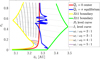 |
Fig. 2 Resonance structures (equilibriums and libration width) of the integrable approximation |

3.1.2 Resonance structure of the integrable approximation  for the ν5 resonance
Similar to  , the partial normal form
  is again a 1-DOF system with a parameter J1, and ψ2 ≈ θ2 representing the ν5 resonance angle. For fixed J1, the dynamics of
  is known completely by the level curves of
  , which coincide with the phase flows on the (J2, ψ2) plane. However, the phase plane structure now depends on the normalization order n. In this paper, we carry out the normalization algorithm to order four. Moreover, we define a simplest ideal resonance model, denoted as
  , by
, by
 (20)
(20)
Figure 3 presents the phase portraits of  with n = 0, 1,…, 4 for a particular value of J1. We find that: the stability of the two equilibriums located at ψ2 = 0 changes as the normalization order increases from zero to two and remains the same for n = 3, 4; (2†). A new center at ψ2 = π appears in frame c for n = 2, disappears in frame d for n = 3, and reappears in frame e for n = 4.
First, we recall that the level curve of J1 is almost vertical, and the larger (smaller) the value of J2 ≈ I2 = P2, the larger (smaller) the eccentricities. In fact, the level curve of J1 adopted in Fig. 3 is located at a1 ≈ 3.17 AU; and the upper (lower) bound of J2 in Fig. 3 corresponds to e1 ≈ 0.55 (e1 ≈ 0.27). From Fig. 2, one may see that the lower bound of J2 is touching the yellow left boundary of the J2:1. Second, we note that the closer to the libration boundary of J2:1, the slower the Fourier expansion Eq. (10) converges (see Fig. B.4). So, the phenomenon (1†) above actually indicates the necessity of the normalization algorithm when close to the J2:1 libration boundary: the qualitative difference between frames a and b in Fig. 3 indicates that the strength of the harmonics of the form cos (lψ2) is so strong that they cannot be simply ignored. Moreover, the phenomenon (2†) indicates that when too close to the libration boundary, a low-order truncation of the partial normal form (such as to order four) is not convincing.
Further, it is necessary to show that when not too close to the J2:1 libration boundary, the low-order normal form is asymptotic, that is, (1*) the structures of the normal form truncated at low orders such as order four indeed reflect properly the original dynamics of  ; (2*) the accuracy of the normal form increases as the normalization order increases. This part of work is tedious and saved in Appendix E, where we computed the surfaces of section of the systems
  and
and  to show (1*), and verify (2*) by numerical integration of example orbits.
We move on to the global structures of the ν5 resonance inside the J2:1. For fixed J1, we determine the locations of the equilibrium on the phase portrait and its stability for  with n = 0, 1,…,4. For centers (if exist) located at ψ2 = ψ2,c with ψ2,c = 0, or, π, we determine its libration width by finding the two intersection points of the largest libration orbit with the section ψ2 = ψ2c. So, both the locations of centers and the libra-tion boundaries are presented by one-dimensional curves in the (J1, J2) plane. Moreover, instead of the (J1, J2) plane, it is more intuitive to present the resonance structures on the
  plane as in Fig. 2. To realize this, for a point (J1, J2) at the section ψ2 = ψ2,c, we conduct the transformation5
 (21)
(21)
and solve  from
from  . The results are presented in Fig. 4.
In each frame of Fig. 4, equilibriums of the ideal resonance model  located at ψ2 = 0 (ψ2 = π) as well as the resonance width are presented as solid red (blue) curve as a reference for comparison. The resonance center of the normal form
  with n = 1,…, 4 located at ψ2 = 0 (ψ2 = π) is presented as dashed red (blue) curves in frames a-d. In frame a, there exist qualitative differences for centers at ψ2 = 0, which correspond to the phenomenon (1†) mentioned earlier. This again indicates the non-negligible strengths of the harmonics cos (lψ2) with l ≥ 2 in the Fourier expansion and the necessity of the normalization procedure. However, it is interesting to find that the structures of the ideal resonance model agrees well with those of the normal form
  as shown in frames b-d, except the structures for centers at ψ2 = π close to the left boundary of the J2:1 resonance (the black dashed curve). As mentioned earlier by the phenomenon (2†), the structures close to the libration boundary are suspicious because of the slow convergence (or simply divergence) of the normal form when the Fourier expansion converges slowly. In fact, results of the surfaces of section in Appendix E shows that the suspicious structures do not exist in the original systems
  and
and  and are thus fictitious. The boundaries of libration domain of ν5 resonance are presented in Fig. 4 as pink (light blue) curves for centers at ψ2 = 0 (ψ2 = π)·We note that libration boundaries for the suspicious centers identified earlier are not presented here.
As shown in Fig. 4, the phase location of the v5 stable centers exhibits two shifts as  increases: the first one from ψ2 = 0 to ψ2 = π occurs at
  , and the second one from ψ2 = π to ψ2 = 0 occurs at
  . We note that only the second one is reported in Morbidelli & Moons (1993), where in their Fig. 3, though not stated clearly, the locations of unperturbed equilibrium of v5 resonance (namely results of K0(J) in Eq. (20)) are presented by a smooth curve there instead of the perturbed equilibriums presented here.
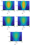 |
Fig. 3 Phase portraits of the integrable approximation |

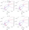 |
Fig. 4 Locations of v¡ resonance centers and the corresponding boundaries of the libration domain of the partial normal form |


3.2 Numerical computation of pseudo-proper elements
For an orbit of the complete system ERTBP, supposing it is trapped in the v5 resonance, to determine its location in the libration domain in Fig. 4 is equivalent to the determination of its proper elements using the perturbation scheme developed in Sect. 2. That is, for an initial condition in terms of the chart (P, Q), we calculate  ; then, the proper element (J1,pro, J2,pro) is given by the intersection point of the flow determined by (J,ψ) with the section ψ2 = 0, or, π. Using Eq. (21), we obtain the proper element
  , from which (a1,pro, e1,pro) is solved, and can be projected onto Fig. 4. To conclude, the proper element is defined as the intersection of the flow of the system
  with the section
 (22)
(22)
An alternative approach is to define the so-called pseudo-proper elements (e.g., Roig et al. 2002) by numerically integrating the flow and recording intersection points using sections equivalent to (or close to) Eq. (22). To be more specific, the pseudo-proper elements can be generated using the following criteria suitable for different systems
 (23)
(23)
As a first example, the yellow dots6 in frame c of Fig. 4 present the pseudo-proper elements of the orbit of the system  presented in frame c of Fig. E.1. The initial condition corresponds to a v5 resonance center provided by the normal form of order three. As expected, the projection of the pseudo proper elements dwells exactly on the dashed blue curves instead of the solid blue curve. As noted in footnote 5, the Lie mapping ℒ3, although a near-identity transformation, is non-negligible for an agreement between the yellow dots (pseudo-proper element) and the dashed blue curve (curve of resonance center of normal form) observed in frame c.
Next, we used the SWIFT package (Levison & Duncan 1994; Brož et al. 2011) to carry out a more systematic computation of the pseudo-proper elements. In this way, we completed the test of the first chain of the perturbation scheme in Fig. 1 by directly comparing the system  . First, we generated a grid
  that covers the libration domain of the J2:1 as shown by black crosses in Fig. 5. Using the relations in Eq. (2), we derive the corresponding
  from
from  . Then, fixing that
  and
and  , or, π, we obtain the corresponding (P, Q)(i,j) from
  using ℒ1 under the condition that Q3 = Q4 = 0. In this way, we obtained two sets of initial conditions that both cover the libration domain of the J2:1. One set satisfies ɡ1 − ɡ2 ≈ 0 and the other set ɡ1 − ɡ2 ≈ π. Then, the two sets of initial conditions are numerically integrated using the SWIFT package for 1 Myr to record its pseudo-proper elements using the first criterion for HpERTBP in Eq. (23). The results are presented as dots in Fig. 5. As shown in Fig. 5, for orbits whose initial conditions are outside the ν5 libration domain, the gray dots generally coincide with the black crosses as expected. For orbits initially dwelling in the ν5 libration domain (colored dots), there are two clusters of pseudo-proper elements that are distributed on the two sides of the curve of ν5 resonance center along the level curves of I1 ; and one of the two clusters coincide with the black crosses. The initial conditions that have no results of pseudo-proper elements correspond to very unstable orbits that escape the J2:1 within a short-time interval.
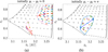 |
Fig. 5 Pseudo-proper elements (dots) of orbits inside the J2:1 commen-surability obtained by the SWIFT package. The black crosses mark their initial conditions with 𝑔1 – 𝑔2 ≈ 0 (𝑔1 – 𝑔2 = π) in the left (right) frame. The section Q2 ≈ 0 (Q2 ≈ π) in Eq. (23) is used to record the pseudo-proper elements of each orbit in frame a (frame b). The colored (gray) dots mark the pseudo-proper elements of orbits trapped (not trapped) in the v5 libration domain. |
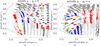 |
Fig. 6 Drifts of pseudo-proper elements of orbits inside the J2:1 commensurability due to the diurnal Yarkovsky effect. The initial conditions are the same as those in Fig. 5 while the Yarkovsky effect is included in the force model (see the text for physical parameters related to the Yarkovsky effect). As in Fig. 5, the section Q2 ≈ 0 (Q2 ≈ π) in Eq. (23) is used to record the pseudo-proper elements of each orbit in frame a (frame b). The integration time is 2 Myr. The ν5 resonance structures are taken from Fig. 4. The gray curves are the level curves of I1 that the ν5 libration approximately follows. Compared with Fig. 5, the pseudo-proper elements show obvious systematic drifts. The light yellow curves in frame a mark the pseudo-proper elements obtained using partial normal form H2* perturbed by |

4 Drifts in the action space of the J2:1 resonance by the Yarkovsky effect
4.1 Classification of systematic drifts by numerical simulations
We started by running numerical simulations using the two sets of initial conditions in Fig. 5 and the augmented version of the SWIFT package by Brož et al. (2011), which supports the option of the Yarkovsky effect in the force model. The physical parameters for the Yarkovsky effect are chosen as R = 0.5 m, ω = ω(R = 0.5 m), ρ = ρreg, K = 10−6 W/ (m K), C = Crock (see Eq. (D.5)), and θ0 = 0, that is, all asteroids are assumed to be prograde rotators. Then, we record the pseudo-proper elements of each orbit during 2 Myr integration (using the section for HpERTBP in Eq. (23)) and present the results in Fig. 6 in the same pattern as in Fig. 5.
Compared with Fig. 5, it is clear that the pseudo-proper elements show systematic drifts because of the Yarkovsky effect. The drift patterns can be generally classified into four types:
Type Ia (Light gray dots): the orbits are not trapped in the ν5 resonance and the drifts are almost parallel to the level curves of I1 ;
Type Ib (Dark gray dots): the orbits are not trapped in the ν5 resonance and the drifts cross the level curves of I1 ;
Type IIa (colored dots except red/blue): the orbits are trapped in the ν5 resonance and the drifts are almost parallel to the ν5 resonance curves;
Type IIb (red and blue dots): the orbits are temporarily trapped in the ν5 resonance during the integration and the drifts are almost parallel to the level curves of I1 but “jumps” over the ν5 libration domain.
To better understand the above classifications, Fig. 7 presents for each type an example trajectory on the plane (ɡ1 − ɡ2 , e1). Frame a presents two orbits of Type Ia marked as gray dots with black edges in the left frame of Fig. 6: the upper (lower) panel corresponds to the orbit with  . The ν5 resonance angle ɡ1 − ɡ2 is in circulation with d/dt (ɡ1 − ɡ2) < 0 for both orbits while the peak of eccentricity is located at ɡ1 − ɡ2 = π and ɡ1 − ɡ2 = 0 for the upper panel and the lower panel, respectively (The reason is easily explained using the ν5 resonance portrait for the corresponding I1 value of each orbit). For this reason, the orbits with larger J2:1 resonance libration amplitudes appear to drift faster because the section to record pseudo-proper elements is chosen as ɡ1 − ɡ2 = 0 in the left frame of Fig. 6. The same phenomenon exists in the right frame of Fig. 6 as shown by the two orbits marked by gray dots with edges. However, the situation is converse now: the orbits with smaller libration amplitude appear to drift faster because the section to record pseudo-proper elements is chosen as ɡ1 − ɡ2 = π. We may conclude that for Type Ia drifts, the pseudo-proper semi-major axis does not change much, and the drift rate of the eccentricity has a weak dependence on the J2:1 resonance libration amplitude.
Frame b presents two orbits of Type IIa where the top (bottom) panel corresponds to the yellow (brown) dots in the libration domain of Ψ2 = 0 (Ψ2 = π) with  in the left (right) frame of Fig. 6. It is clear that ɡ1 − ɡ2 is in libration for both orbits. The difference is that in the upper panel the libration cycle is going up while in the lower panel the libration cycle is going down as marked by the arrows. In fact, the common characteristic for drifts of Type IIa in Fig. 5 is that they all move in the leftward direction in the pseudo-proper a1 − e1 plane with the footprints almost parallel to the v5 resonance curve. So, for an orbit trapped in the v5 libration domain with centers located at Ψ2 ≈ g1 − g2 = 0 (namely the regions encircled by the pink curves) at about 3.17 AU, its eccentricity would increase as it drifts parallel to the resonance curve in the leftward direction. On the other hand, for an orbit trapped in the libration domain encircled by pink curves at about 3.25 AU, its eccentricity would decrease. For orbits trapped in the v5 libration domain encircled by the light blue curves, its eccentricity would always decrease.
Frame c presents an orbit of type Ib, which corresponds to the dark gray dots with black edges located at the top of the left frame of Fig. 6. From frame a of Fig. 6, the orbit approaches the stable libration boundary of J2:1 as the pseudo-proper semimajor axis decreases due to the Yarkovsky force while the eccentricity does not show obvious growth. Frame c shows that g1 − g2 is in circulation with d/dt (g1 − g2) > 0 under the Yarkovsky force. As the orbit hits the boundary, the close encounter with Jupiter changes its semi-major axis and eccentricity abruptly. Then, the eccentricity undergoes large-amplitude oscillation due to secular resonances.
Frame d presents two orbits of Type IIb where the top (bottom) panel corresponds to red (blue) dots at 3.25 AU (3.18 AU) in the left frame of Fig. 5. Both orbits start at the section g1 − g2 = 0, and its evolution exhibits three phases: The first phase is marked by the arrow 1, during which g1 − g2 is in circulation with d/dt (g1 − g2) < 0 and the eccentricity increases slowly, namely the Type Ia drift. The second phase is marked by the arrow 2, during which the orbit is temporarily trapped in v5 resonance, and the eccentricity increases rapidly during one incomplete cycle of the v5 libration. The last phase, marked by arrow 3, is again a Type Ia drift in which the g1 − g2 is in circulation with d/dt (g1 − g2) > 0 and the eccentricity increases slowly. Intuitively speaking, the orbit of Type IIb jumps over the libration domain under the Yarkovsky effect and gains a rapid increase of eccentricity as a result.
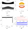 |
Fig. 7 Trajectories on the (e 1,ɡ1 − ɡ2) plane for example orbits of different types of drift identified in Fig. 6. Frame a presents two orbits of Type Ia marked as gray dots with black edges in the left frame of Fig. 6; Frame b presents two orbits of Type IIa dwelling in the libration domain of Ψ2 = 0 (Ψ2 = π) at |


4.2 Analysis on the drift rates of pseudo-proper elements
We compute in Sect. 2.5 the averaged values of the differentiate rates of J1, J2 due to the Yarkovsky force, namely  . Our goal is to link
  with the drift rates of the pseudo-proper semi-major axis and eccentricity, namely
  and explain the different types of drifts observed in the previous section.
Before moving on, it is necessary to first show that the several types of drifts identified above indeed exist in the nor- malized systems  under the perturbation of the averaged Yarkovsky force
  . So, we integrate the initial conditions of several orbits in Fig. 6 using the canonical equations of H2* perturbed by
  and record the pseudo-proper elements, which are presented in the left frame of Fig. 7 using small light yellow dots (which appear as thin yellow curves). It is shown that the yellow dots agree well with the corresponding colored dots. This suggests that the dynamics that interests us is preserved in the normalized system with the averaged Yarkovsky force.
With Eq. (21), we defined two tabulated functions a1,pse (J1,pse, J2,pse), and e1,pse J1,pse, J2,pse) on a grid in the action space J1 − J2 . Then, the differentiation of the two functions bridges the drift rates of (a1,pse, e1,pse) and that of J1,pse, J2,pse). Because J1,pse is a parameter of the partial normal form  , we have J1,pse = J1 and thus
  .
.
We recall by definition that J2,pse satisfies the relation H(J2,pse,Ψ2 = 0; J1) = h. So we write J2,pse = J2,pse(J1, h), for which the differentiation gives (similar to Eq. (16))
 (24)
(24)
For applications, we should average Eq. (24) over one cycle (libration or circulation) of the v5 resonance, namely  , where Tv5 is the period of the v5 resonance. We note that the two cases of the integration trajectory, namely circulation and libration, correspond to the Type I and the Type II drifts, respectively.
Since  is very small, the averaging can be carried along a flow of the normal form without considering the effects of
  . That is, J1 and h are assumed as constants in the right-hand side of Eq. (24). So, the variations of
  during one cycle of v5 resonance is subject only to the oscillation of J2 . The contour maps of
  (not shown here for simplicity) shows that (1) the variation of
  is small for fixed a1 (which can approximate the level curve of J1 along which the v5 libration follows); (2) the variation of
  is small in the whole J2:1 libration domain. So, it is reasonable to assume that
  is constant during one cycle of v5 resonance so that
 (25)
(25)
4.2.1 Type Ia drift
Consider again the relation H(J2,pse,Ψ2=0;J1)=h. Taking J2,pse as a function of h and J1 , the differentiation of the formula gives
 (26)
(26)
In the case that the Ψ2 is in circulation and away from the libration domain, the variation of J2 is small during one cycle so that ∂H/∂J1≈〈∂H/∂J1〉. Then Eq. (26) implies that the first term in Eq. (25) proportional to  vanishes. Moreover, we clearly have
  for circulation flows. Since the variation of J2 is small we can further estimate that
  . So in the case of Type I drift, Eq. (25) is rewritten as
 (27)
(27)
Using Eq. (27), we obtain the vector filed υc = (daı,pse/dt, de ı,pse/dt) in the circulation domain of the v5 resonance. We note that the vector field υc(a1,pse, e1,pse) is not known explicitly, but it can be calculated on a uniform grid. In this way, for any location inside the grid, υc can be obtained by interpolation, and the Type I drift corresponds to the integration trajectory of the vector field.
The strength-normalized vector field υc/||υc|| for Type I drift is presented in Fig. 8, which is superimposed with footprints (marked by colored dots) of some example orbits obtained by numerical integration of  perturbed by
  . In Fig. 8, the green curves are integration results of the vector fields υc using the same initial conditions of the example orbits. We note that the deviations between the colored dots and the green curves for the two Type Ia drifts (namely the red and the pink circles) are due to the periodic oscillations of v5 circulation as presented in frame a of Fig. 7. For the two Type Ib drifts (namely the yellow and the purple circles), the results agree well, though the drift rate of the pseudo proper a1 shows some deviation for the orbit with
  (the purple circle).
As expected from its definition in Sect. 4.1, the vector field υc for Type Ia drift is almost parallel to the level curves of J1 . So, it is reasonable to assume that J1 is constant for Type Ia drift and only consider the slow variation of J2 . Moreover, since the strength of  can be considered as being constant, as pointed out earlier, the problem is reduced to the standard case of 1-DOF system with a slowly varying parameter with a constant rate. This simplification has two direct applications. The first is that for Type Ia drift with small J2:1 libration amplitudes at small eccentricities, the problem can be treated analytically instead of semi-numerically as in Sect. 2 because the classical expansion of the disturbing function is valid in this case. See Appendix F for more details on the analytical treatment for this simplified case, which shows that for prograde (retrograde) asteroids, the eccentricity shows a systematic increase (decrease) while the J2:1 libration amplitude decreases (increases).
The second application is a fast estimate on the eccentricity growth rate of Type Ia drift. This comes from two more observations: (1) the eccentricity growth rate is insensitive to the J2:1 libration amplitude as seen from the two green curves for Type Ia drifts in Fig. 8; (2) for Type Ia drift the semi-major axis can be considered as constant since the level curve of J1 is almost vertical. So by simply focusing on the Type Ia drift along the J2:1 libration center that is located approximately at a1,c ≈3.27 AU, the eccentricity growth is determined by integrating the differential equation
 (28)
(28)
Using Eq. (28), it is straightforward to find the eccentricity excitation time TIa(e1, i, e1, f )for Type Ia drift as
 (29)
(29)
Once e1,i and e1,f are given, the value of TIa(e1,i,e1,f) only depends on  , which in turn relies on the input of the physical parameters of the diurnal Yarkovsky effect. Figure 9 presents the contour map of TIa (e1,i, e1,f) on the K − ρ plane while fixing D, Tspin. We note that Fig. 9 has similar profiles as Fig. 4 of Fenucci et al. (2021) where the semi-major mobility due to the Yarkovsky effect outside the mean motion resonance is considered.
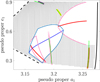 |
Fig. 8 Strength-normalized vector field υc/||υc|| on the pseudo-proper a1 − e1 plane for Type I drifts. The colored circles are footprints of Type I ∗ drifts obtained by numerical integration of the partial normal form |


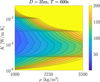 |
Fig. 9 Contour map of the eccentricity excitation time TIa (e1,i, eı,f) for Type la drift in the J2:1 commensurability. The unit of TIa (e1,i, e 1,f) is Myr with e1,i = 0.2 and e1,f = aJ/aJ2:1 − 1 ≈ 0.59. The diameter D of the asteroid is fixed as 35 m, and the spin period is fixed as 600 s. |
4.2.2 Type IIa drift
In case of libration, the relation Eq. (25) is singular because  . To fix this problem, we introduce the action variable Θ for the partial normal form
  , that is,
  . Since Θ = Θ (J1, h), we replace h by Θ in Eq. (27) such that
 (30)
(30)
Similar to Eq. (16), we have
 (31)
(31)
and Eq. (31) could be averaged over one libration cycle of v5 resonance similar to Eq. (25). However, assuming that Θ is an adiabatic invariant, that is dΘ/dt ≪ 1, we could simplify Eq. (30) as
 (32)
(32)
The adiabatic assumption of dΘ/dt ≪ 1 implies that the drift of pseudo proper a1 − e1 is along the level curve of Θ. To compute ∂J2,pse (J1, Θ)/∂J1, we first generate a non-uniform grid (J2,(i,j), J1,j) in each v5 libration domain, and compute Θ on each node of the grid. In this way, we obtain a tabulated function J2 (Θ, J1) defined on the non-uniform grid (Θ(i,j), J1,j). Then, ∂J2 (Θ, J1)/∂J1 is obtained by interpolation and numerical differentiation of J2 (Θ, J1).
Using Eq. (32), we obtain the vector field υl = (da1,pse/dt, de 1,pse/dt) inside the three libration domains of the v5 resonance. Fig. 10 presents separately the strength- normalized vector field υl /||υl| in each libration domain. Each frame is superimposed with the footprints (colored circle) of a Type IIa drift, which is obtained by numerical integration of  perturbed by
  , and the numerical integration result (green curve) of the vector field υl . It is shown that the green curves agree well with the reference results of colored circles, which suggests the validity of the adiabatic assumption of Θ.
Compared to Type Ia drift for which  plays the key role (Eq. (27)), the Type IIa drift is mainly subject to
  (Eq. (32)), which requires an extra averaging over the J2:1 cycle besides the Schubart averaging over the mean motions. So, for simplicity, we do not perform similar computation as in Fig. 9 for Type IIa drifts here.
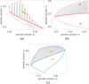 |
Fig. 10 Strength-normalized vector field υl/||υl|| in the three libration domains of v5 resonance on the pseudo-proper a1 − e1 plane. The colored circles are footprints of Type IIa drifts obtained by numerical integration of the partial normal form |


5 Discussion
In the above analysis, we have assumed that the spin of the asteroid is prograde. For the retrograde case, the direction of the Yarkovsky force is reversed, and consequently the vector fields for the Yarkovsky-driven drifts also reverse their directions. For Type I drift, we would expect that the eccentricity shows a systematic decrease. Moreover, according to Appendix F, the libration amplitude of J2:1 would increases for retrograde asteroids. So, a possible evolution path for retrograde asteroids subject to Type I drift is the escape from the J2:1 through the left boundary (with smaller semi-major axis) as its eccentricity decreases, and a further migration toward the Sun as its semimajor axis continues to decrease due to the Yarkovsky effect after its escape from the J2:1 resonance.
On the other hand, Henrard et al. (1995) showed that there exits a bridge between the chaotic region caused by the overlap of secondary resonances at small eccentricity (low-e region) with the chaotic regions caused by the overlap of secular resonances at large eccentricity (high-e region); and for moderate inclinations, this bridge is “open” only to orbits with large enough J2:1 libra-tion amplitudes. Moreover, they mentioned that it is difficult for orbits to diffuse from initially small libration amplitude to large amplitude to take this bridge, and no such orbits were found in that paper where only gravitational effects were considered. Nevertheless, in our study it it is possible that the Yarkovsky-driven drifts for retrograde asteroids may serve as a mechanism to drive the asteroids to the bridge. So, a second evolution path for retrograde asteroids subject to Type I drift might be an escape from the J2:1 resonance through the bridge from small eccentricities to large eccentricities.
We find that the two evolution paths described above can both be found in numerical simulations. Figure 11 presents four example orbits7. The initial conditions dwell in the J2:1 libra-tion domain with initial pseudo-proper eccentricities at about 0.2. The simulation is then carried out using the SWIFT package (Levison & Duncan 1994; Brož et al. 2011) where the force model includes the four planets: Jupiter, Saturn, Earth, and Mars.
The integration time is 100 Myr and the integration is stopped whenever the asteroid hits the Sun or escapes outside 10 AU from the Sun. The upper (lower) three frames of Fig. 11 present the evolution without (with) the Yarkovsky effects8. The left column presents the time evolution of osculating a1, e1 and i1 while the middle (right) column presents footprints on the pseudo-proper a1 − e1 plane (osculating e1 − i1 plane).
From the first panel of frame a and frame b without the Yarkovsky effect, all four orbits are confined to the J2:1 libration domain throughout the evolution. In terms of the eccentricity, the brown (green) orbit diffuses into the low-e region with e1,min ≈ 0 (e1,min ≈ 0.1). In terms of the inclination, as seen from the last panel in frame a, all four orbits increase to moderate values of about 20° (the mechanism behind may be some inclination-type secular resonance that causes long-period large-amplitude oscillations of inclinations). Moreover, an important phenomenon by the brown orbit is that the inclination increases from 30° to 60° after T = 70 Myr during its slow diffusion in the low-e region. We note that this phenomenon - increase of inclination during the diffusion in the low-e region - has been pointed out by Henrard et al. (1995) and it was proposed therein that the possible mechanism behind might be a resonance between the frequency of the secondary resonance and the planetary frequency s6. We choose not to perform a further analysis of the mechanism behind this phenomenon here for simplicity while it obviously deserves further investigations.
The lower three frames present the two evolution paths described above when the Yarkovsky force is in effect: as shown in frame d, the brown orbit takes the first path to escape from the J2:1 with a small eccentricity while the other three orbits take the second path to escape with large eccentricities. It is clear from the second panel of frame d that all four orbits exhibits a systematic decrease of eccentricities before 40 Myr. The escape of the brown orbit through the left boundary of J2:1 indicates that the J2:1 libration amplitude increases due to the Yarkovsky force. For the three orbits (blue, purple, and green) that take the second path, the orbits also get closer to the libration boundary of the J2:1 resonance (e.g., for fixed pseudo-proper e1 = 0.2, the minimum pseudo proper a1 is about 3.21 AU in frame e, smaller than 3.23 AU in frame b). The systematic decrease of eccentricities force them to go deeper into the low-e region, and as a consequence, their inclinations all diffuse into moderate values because of the mechanism related to the secondary resonance. It is then clear from frames d and f that the increase of eccentricities occur after the orbits reach moderate values of inclination, and it is also clear from e that the entrance into the high-e region occurs with large J2:1 libration amplitudes. So it is reasonable to argue that these orbits take exactly the bridge proposed by Henrard et al. (1995) with the help of the Yarkovsky force. After entering the high-e region, the secular resonance leads to large-amplitude oscillations of eccentricities and inclinations, as shown in frame f.
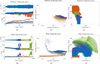 |
Fig. 11 Evolution trajectories of four example orbits to show the evolution paths of retrograde asteroids inside the J2:1 resonance. |
6 Conclusion
In this paper, we have investigated the interaction between the Yarkovsky effect with the J2:1 resonance as well as the v5 secular resonance inside J2:1 under the model of the planar ERTBP. The resonance structures inside J2:1 were revisited using the semi-analytical perturbation methods following previous researches, while two complements have been presented here:
We complemented the extended Schubart averaging developed in Moons (1994) by computing the canonical transformation that bridges the original system and the averaged system.
We carried out higher order normalization (to order four) of the Hamiltonian for the v5 integrable approximation compared to the pioneering work by Morbidelli & Moons (1993).
After revisiting the resonance structures, a perturbative treatment of the systematic drifts in the action space of the J2:1 due to the Yarkovsky effect was carried out. The averaged diurnal Yarkovsky effect that can be applied to the normal form of the Hamiltonian was obtained using the chain of canonical transformations. Then, the drift rates of the pseudo-proper elements were derived from the analysis of the normal form perturbed by the averaged Yarkovsky force. Our main results are the following:
We identified two main types of systematic drifts in the action space: (Type Ia) for orbits not trapped in the v5 resonance, the footprints are parallel to the resonance curve of the stable center of the J2:1 resonance; (Type IIa) for orbits trapped in the v5 resonance, the footprints in the action space are parallel to the resonance curve of the stable center of the v5 resonance.
For the Type Ia drifts, we proposed a fast algorithm to compute the Yarkovsky-driven excitation of the orbit eccentricity. For Type Ia drifts with small oscillations around the J2:1 center and small eccentricities, we carried out an analytical treatment and showed that for prograde (retrograde) asteroids, the eccentricity shows a systematic increase (decrease) while the J2:1 libration amplitude decreases (increase).
A vector field in the action space, of which the integration trajectory corresponds to the systematic drift induced by the Yarkovsky force, was derived.
With the help of the Yarkovsky-driven decrease of eccentricity and the increase of the J2:1 libration amplitude, retrograde asteroids may be driven to the bridge that connects the secondary resonance and the secular resonance. Numerical simulation showed that the escape of retrograde asteroids from the J2:1 resonance through this route is a possible effect pending future investigations.
Acknowledgements
This work is supported by National Natural Science Foundation of China (No. 12233003).
Appendix A Schubart averaging
A.1 Explicit formula of ∂H/∂σR
In this appendix, column vector is assumed by default. First denote three element charts — the Keplerian chart, the Delau-nay chart, and the resonance chart suitable for J2:1 resonance as
 (A.1)
(A.1)
where  , and the superscript t refers to transpose of the vector. The goal of this appendix is to derive the explicit expressions of
  as well as
  . The partial derivatives with respect to σR of the first four terms of
  in Eq. (3) are simple. The difficulty lies on the perturbation part proportional to m2
 (A.2)
(A.2)
For ∂R/∂σR, we first note the following chains of partial derivatives
 (A.3)
(A.3)

and from Eq. (2)
 (A.5)
(A.5)
Notice that when e1 = 0, we have  so that the transformation
  in Eq. (A.3) is singular. To eliminate this geometrical singularity, one may consult the nonsingular variables (e.g., Moons 1994) instead of the Keplerian chart here. Nevertheless, for our problem, the result based on the Keple-rian chart is sufficient. Now, to write ∂R/∂σR, all we need is ∂R/∂σK. This is developed as follows. Considering the case of planar ERTBP, we have
 (A.6)
(A.6)

It is then straightforward to derive from Eq. (A.7) the following
 (A.8)
(A.8)
 (A.9)
(A.9)
 (A.10)
 (A.11)
To derive expression of ∂I/∂σK, first transform the true anomaly to the eccentric anomaly using the third and the fourth of Eq. (A.7). The rest is straightforward. However, the result is quite long and not presented here for simplicity. At last, for the term D, we have the following identities
 (A.12)
The next is to use Eq. (5) to evaluate the time average  and
and  . Because
  is explicitly expressed in terms of the eccentric anomaly E1 and E2, to compute the right-hand side of Eq. (5), two Kepler equations must be solved at every step. A trick that allows one to solve only one Kepler equation is to use the following two relations (Moons 1994)
 (A.13)
which can be derived from Eqs. (A.7) and (2). Using Eq. (A.13), the averaging in Eq. (4) can be rewritten as
 (A.14)
A.2 Short-period term corresponding to mean motions
The averaged system obtained by averaging over Q3 is linked with the original system through the short-period terms, which can be evaluated (to some precision) using the first-order perturbation theory. To derive it, first sort the Hamiltonian function H (Q, P) as
 (A.15)
The reason to include the Kepler term for m1 in H1 is that when near the p + q : p resonance, the variation of the first two terms of H1 is of order O(m2), that is, when ignoring a constant term, the magnitude of the first two terms of H1 is of order O(m2).
The generating function W to remove the short-period term is determined by the homological equation (for more on the Lie transform method, one may refer to Appendix B.4)
![$\matrix{ { - \left\{ {{H_0};W} \right\} = {{\partial {H_0}} \over {\partial {P_3}}}{{\partial W} \over {\partial \lambda }} = H - \bar H,\quad \bar H = {1 \over {2p\pi }}\mathop \smallint \limits_0^{2p\pi } Hd{Q_3}} \hfill \cr {\left[ {\left\{ {f,g} \right\} = \mathop \sum \limits_{i = 1}^4 {{\partial f} \over {\partial {Q_i}}}{{\partial g} \over {\partial {P_i}}} - {{\partial f} \over {\partial {P_i}}}{{\partial g} \over {\partial {Q_i}}}} \right].} \hfill \cr } $](/articles/aa/full_html/2024/09/aa49770-24/aa49770-24-eq269.png) (A.16)
(A.16)
To solve Eq. (A.16), we need the explicit form of  We may conduct a Fourier expansion of Φ as
  . Using the orthogonal properties of trigonometric functions, we have
 (A.17)
Supposing that ak, bk are already solved, then Eq. (A.16) is solved as
 (A.18)
The Lie mapping 𝓛1 in Eq. (6) is then generated by W as
 (A.19)
which requires ∂αk/∂σR,∂bk/∂σR, which from Eq. (A.17) are given by
 (A.20)
Note that  as easily seen from Eq. (A.17). We mention that the averaging in Eq. (A.20) is also transformed into a Riemann sum.
Appendix B Technical details on Morbidelli’s elimination of harmonic and partial normalization
B.1 Preliminaries: Analysis of the integrable approximation of the J2:1 resonance
For the Sun-Jupiter system, according to Kepler’s third law  , the 2:1 commensurability n1/n2 = 2 is located at
  his appendix, we focus on a rectangular region S1 in the space a–e determined by 3.0616 ≤ a1 ≤ 3.3389, 0.001 ≤ e1 ≤ 0.549. Using Eq. (2), the rectangle is projected onto a region S2 in the
  . We generate a grid 𝒢1 in the region S2 (see the grid consisting of dark crosses in the left frame of Fig. B.1)
 (B.1)
(B.1)
We note that the grid 𝒢1 is nonuniform in the sense that it is not equivalent to a product of two arrays such as  ever, it is not a random grid because the P2 coordinate depends only on the index j. The projection of the grid 𝒢1 onto the a1 − e1 plane is again a nonuniform grid because of the non-linearity of the transformation; see the grid of dark crosses in the right frame of Fig. B.1.
At each node  , for arbitrary value of
  , the function
  can be evaluated using Eq. (8). Since J2:1 is of first-order resonance, its equilibrium is located at
  , or, π. Two typical phase portraits of
  for different
  ( equivalently different values of eccentricity) are presented in Fig. B.2. There are two notable phenomena: (1) for small eccentricities, there exists no saddle point at
  (Morbidelli 2002); (2) for moderate and large eccentricities, the Schubart averaging result becomes unstable in the neighborhood of collision curves, which corresponds to the configuration in which the eccentric orbit intersects Jupiter’s orbit. In this case the Schubart averaging suffers from the singularity at ∆ = 0.
We shall focus on the dynamics in the libration domain of J2:1 resonance. For this purpose, we need to determine the locations of its resonance center and libration boundaries. Fixing the parameter  ·, the resonance center (saddle) can be determined by finding the point where
  attains maximum (minimum) along the section
  . In Fig. B.1, the red (blue) curve presents the locations of resonance centers (saddles). We note the lack of the saddle curve at small eccentricities and and the irregularity at the large eccentricities are due to the two phenomena mentioned above.
For a given  , the libration boundaries are defined as the maximum and minimum values of
  along the largest libration orbit, or equivalently the two intersection points of the largest libration orbit with the section
  . When the saddle point exists, the separatrix can be considered as the largest libra-tion orbit. However, since saddle point is not always available, we find the largest libration orbit (to some precision) by integrating initial conditions that are gradually away from the resonance center.
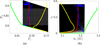 |
Fig. B.1 Left frame: Grid 𝒢1 marked by black crosses, which is the work domain for the integrable approximation |


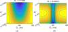 |
Fig. B.2 Two typical phase portraits of the integrable approximations |


To avoid the precision loss of Schubart averaging at large eccentricity in the neighborhood of the collision curve, we constrain that the minimum distance from Jupiter should be larger than 10−2a2 = 0.052AU. In Fig. B.1, the green and the yellow curves correspond to the two libration boundaries. As a result of our setting, the libration domain shrinks as the eccentricity increases for  as shown in Fig. 2.
B.2 Computation of the Arnold action variable and the mapping ℒ2
After the preliminaries above, we compute the action-angle variable (I, θ) of  and the canonical transformation
  in Eq. (6).
Fixing  , for a periodic flow with an initial condition
  and an energy
  , the Arnold action variable I1 is defined as
  , where the function
  is obtained by the inversion of the energy equation. Geometrically, I1 corresponds to the oriented area encircled by the flow. Moreover, using the definition of I1 and the canonical equation of
  , we have ∂I1/∂h = T/2π where
  is the period of the flow. Now, define the angle variable θ1 as θ1 = 2πt/T. The variable change from
  to (I1,θ1) is in fact canonical, and can be generated by the generating function
 (B.2)
(B.2)
Up to now, we complete the definition of action-angle variable for the 1-DOF system  . In order to apply
  to the 2-DOF system
  , we modify S as
 (B.3)
(B.3)
which gives set (a) in the following
 (B.4)
(B.4)
Set (a) is inconvenient to use because of mixing old and new variable. Set (b), which transforms new variables to old ones, namely the mapping of ℒ2, is derived as follows. First, the inversion of the third equation of set (a) directly gives the third of set (b). Substitution of this inversion into the first of set (a) gives the first of set (b). All that is left is the last of set (b), which is known as the Henrard-Lemaitre formula (Henrard 1990; Ferraz-Mello 2007). To derive it, one finds by some calculation that  and replace
  in the integration by
  , which is valid considering that the integration is carried along a flow of
  so that I1, I2 are constants.
So far, we have completed the formal computation of the Arnold action variable and the mapping ℒ2. However, because the explicit expression of  is not available, the computation must be realized in a numerical way, as mentioned in Sect. 2.3. For any point
  dwelling inside the libration domain in Fig. B.1, the coordinate
  uniquely determines a libration flow of
  with the initial condition
  and the parameter
  . Integrating the flow for a period T, we obtain an equally time-spaced ephemeris
 (B.5)
(B.5)
Then, the mapping ℒ2 can be evaluated by interpolation (see Appendix C for necessary details on interpolation methods used in this paper) using the tabulated ephemeris points as follows (Morbidelli 1993)
 (B.6)
(B.6)
where t = Tθ1/2π and ρ (ti) represents the oscillation part of  defined by
 (B.7)
(B.7)
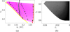 |
Fig. B.3 Frame (a): Projection of the grid 𝒢2 onto the |


The inverse of ℒ2 does not need interpolation but simple integration of the flow
 (B.8)
(B.8)
where t is the time for the flow to travel from the section  to the target point
  . In Eqs. (B.6) and (B.8), all are obvious except transformations using ρ(t), which by Eq. (B.4) should equal the Henrard-Lemaitre formula result. For this, notice that variation of
  determined by
  must take the form of a linear growth with a periodic osculation with period T; also notice that after the canonical transformation in set (b) above,
  so that θ2 varies linearly. Consequently, the Henrard-Lemaitre formula result, which is obviously periodic in θ1, and thus periodic in
  , is just the oscillation part ρ(t).
The above algorithm allowed us to compute the Arnold action variable as well as the mapping ℒ2 for any libration flow with the initial condition  as long as
  dwells in the libration domain in Fig. B.1. However, it is not practical to carry out the above algorithm every time ℒ2 is needed, which would require too much computation time. So, the general idea is to carry out the above algorithm on a grid that covers the libration domain and consult interpolation methods. In the case where ℒ2 is required exactly on a node, applying Eq. (B.6) to the ephemeris of the node would suffice. In the case where ℒ2 is required to not be on a node of the grid, it can be expected that more interpolation work in addition to that in Eq. (B.6) will be required, which we discuss later.
Ideally, we should carry out the algorithm on a regular (Cartesian) grid that covers the libration domain so that the interpolation can be most conveniently performed. However, this is not possible because the libration boundaries are two irregular curves instead of straight lines. So we generated a non-uniform grid
 (B.9)
(B.9)
that covers most of the libration domain. Its projection onto the a − e space is shown as pink crosses in Fig. B.3(a). On each node  of the grid 𝒢2, following the above algorithm, we obtain the equally time-spaced ephemeris ℰi,j, the Arnold action variable
  , equivalently the function
  where
where  , and the period Ti,j. Now, the mapping
  is known on each node of the grid 𝒢2, and naturally the mapping
  is known at each node (I1,(i,j), I2,j) of the grid 𝒢3
 (B.10)
which is presented in Fig. B.3(b).
We return to the problem of determining ℒ2 for a target point (I1,I2, θ1, θ2) with (I1,I2) not a node of the grid 𝒢3. Though it is possible to interpolate ℒ2 using the ephemeris ℰi,j of the nodes that surround (I1 , I2), it requires extra work of Fourier expansion and interpolation. In this paper, we do not carry this part of work, and it turns out that ℰi,j obtained above at each node is enough for our study. We mention one important case here: for θ1 = 0, we always have  no matter the values of I1, I2. In this special case, the mapping ℒ2 can be determined by carrying only a two-dimensional interpolation
 (B.11)
where the tabulated function  is
is
 (B.12)
B.3 Fourier expansion of  in terms of (I, θ)
In this section, we evaluate the two functions  and
and  on each node (I1,(i,j), I2,j), h,j) ∊ 𝒢3. This is possible because at each node of 𝒢3, the variation of the Hamiltonian function
  as θ1, θ2 vary in [0,2π] can be determined using the mapping ℒ2.
There are two alternative ways, and they turn out to be mutually complemented. The first is to assign two artificial frequencies to θ1 , θ2 and generate a long enough sampling signal of  . Then, the amplitude of dominating harmonics can be obtained using the tool of numerical analysis of fundamental frequencies (NAFF, Laskar 2003). The second is to directly obtain the coefficients of a target harmonic by averaging (which is approximated by a Riemann sum). We shall start with the first method to find the harmonics with dominating strengths, and then use the second to compute the coefficients of selected harmonics.
We recall that in the previous subsection, we obtained at each node  (equivalently (I1,(i,j),I2,j) ∊ 𝒢3) a equally time-spaced ephemeris ℰi,j. It is natural to choose the ephemeris points as the sampling point of θ1 (equivalently
  ). Assume that the sampling time interval (the time elapsed between two signals) is ∆t = 1, then the artificially assigned frequency for θ1 is
  . Then, we artificially choose
  so that
  are linearly independent. In this way, we generate a signal set Si,j of
  with totally M data points at the node (I1,(i,j),I2,j) ∊ 𝒢3 as
 (B.13)
where no interpolation is involved. Choosing N = 100, M = 150N, which gives f1 = 10−2, f2 ≈ 6.3661 × 10⁻⁴, we carry the NAFF analysis at the nodes labeled by i = 1,91,181, j = 10,30,50,…, 190, which are marked by dots and crosses in Fig. B.3.
Roughly speaking, the NAFF algorithm starts by finding the frequency of the harmonic with the largest strength in the signal, computes its amplitude, subtracts from the original signal the contribution of this harmonic, and then repeats the above process to find the next harmonic with the second largest strength. We use the NAFF_UV10 software to obtain the frequencies and amplitudes of the first 100 harmonics of the signal at each marked node in Fig. B.3. The NAFF results at the nodes marked by the green dots with black edges are presented in Fig. B.4 (note that the zero frequency term is not shown). Generally speaking, the larger the value of the index i, the closer the node is located to the libration boundary of the J2:1 (namely the yellow curve in Fig. B.3); and the larger the value of j, the larger the eccentricity at the node.
In each frame of Fig. B.4, the red, green and black horizontal lines mark the strengths of amplitude 10−6, 10−7, and 10−8; and harmonics with strengths amplitudes smaller than 10−10 are not shown. Because f1 = 10−2, f2 ≈ 6.3661 × 10⁻⁴, each “bump” in each panel corresponds to a multiple of harmonics of the form k1θ1 + k2θ2 with k1 fixed, and |k2| increasing. For example, in the first frame with (i, j) = (1, 10), only two harmonics have amplitudes larger than 10−6 (above the red line), namely θ2, 2θ2, while five more harmonics have strengths greater than 10−7 (above the green line), namely 2θ2, θ1 ± θ2, θ1 ± 2θ2. From Fig. B.4, one may see that when approaching the separatrix of J2:1 harmonic (namely large j), the Fourier expansion converges very slowly. To truncate the Fourier expansion according to a prescribed threshold σ of amplitude, say σ = 10−7, is to determine a subset 𝒦 of ℤ × ℤ and lmax ∊ ℤ such that  for any (k1, k2) ∊ 𝒦 and l ≤ lmax. However, when fixing σ, 𝒦 and lmax would vary for different points. So, a reasonable way is to select a truncated expansion in prior, and then show that the dynamics of the truncated system as well as the normal form derived from it agree with that of the original system. After some trials, we truncate Eq. (10) by preserving those harmonics satisfying k1 + |k2| ≤ 9, |k2| ≤ 2, lmax ≤ 2. For the validity of this choice, see Appendix E. For the truncated expansion, at each point of the action space, the largest harmonic coefficient σL in the remainder can be used as an indicator for the size of the remainder. The red, blue and yellow dashed curves in Fig. B.3 are three level curves of σL.
For our problem, because the fundamental frequencies are actually known, we do not need the full power of NAFF to determine the coefficient of a target harmonic k1θ1 + k2θ2. This amounts to the second approach, which to some extent requires less computation: the coefficients  for a target harmonic ξ = k1θ1 + k2θ2 can be directly obtained by averaging. First, a point transformation is applied so that
  is expressed in terms of ξ, θ1. Second, an averaging over θ1 is conducted so that all harmonics involving θ1 are eliminated, namely
 (B.14)
We note that the above formula holds because k2 ≠ 0 in the Fourier expansion Eq. (10). Third, the coefficient  is obtained by another averaging similar to Eq. (A.17)
 (B.15)
To evaluate  at the node (i j) , we use the equally time-spaced ephemeris ℰi,j (see Eq. (B.5)) obtained at each interpolation node of the grid 𝒢2 (Eq. (B.9)) to generate a data set S′i,j,· of length K
 (B.16)
Then, the integration Eq. (B.12) is transformed into a Rieman-nian sum using the data set S′i,j as
 (B.17)
 |
Fig. B.4 NAFF results of the sampling signal of |

B.4 Normalization of the Hamiltonian
For a detailed exposition on the Lie transform method, one may refer to Ferraz-Mello (2007). A brief account of the formal computation of the partial normal form  is as follows. To compute the partial normal form using
  as the kernel function, first sort the Fourier expansion of
  in Eq. (10) according to its order of magnitude as follows
 (B.18)
that is, we assume that H0 = O (ε0), and H1 = O (ε) where ε is a small quantity. Suppose that the normalization is carried out to order M, the Lie mapping ℒ3 is generated by a generating function W (J, ψ) as
![${{\cal L}_3}({\bf{J}},{\bf{\psi }}) = \{ ({\bf{J}},{\bf{\psi }});W\} ,\quad \left[ {\{ f,g\} = \sum\limits_{i = 1}^2 {{{\partial f} \over {\partial {\psi i}}}} {{\partial g} \over {\partial {J_i}}} - {{\partial g} \over {\partial {\psi i}}}{{\partial f} \over {\partial {J_i}}}} \right],$](/articles/aa/full_html/2024/09/aa49770-24/aa49770-24-eq380.png) (B.19)
(B.19)
where the generating function W takes the form W = W1 + W2 + … + Wn + …, with Wi = O (εi). The yet determined partial normal form  takes a similar form except a remainder of order n + 1 as presented in Eq. (12). Substituting the series expression of W into Eq. (12), equating terms of same degree after expanding, one arrives at the homological equation that determines Wi recursively from low orders to high orders. The general form of the homological equation of order i reads
 (B.20)
where the last formula is the well-known Deprit’s recursion formula. Assuming that equations of lower orders are already solved, we chose Ki such that the right-hand side of the homological equation is independent of harmonics containing only phase ψ2. For example, for i = 1, 2, we have
 (B.21)
We also note that because  is degenerate, we adopt the simplification that
  .
.
The above procedure of normalization of a Hamiltonian is standard. However, it is inconvenient to realize the procedure using a symbolic manipulator because in our case the Hamiltonian is not known explicitly. Instead, it is known on a tabulated grid, so extra programming efforts are required.
We considered a tabulated trigonometric series f
 (B.22)
in the sense that the coefficients  are not known explicitly, but their values are known for a tabulated grid 𝒢3 of the action space J. First notice that to realize the above procedure of normalization, all we need is to program the operations of sum, product, and Poisson bracket of two trigonometric series f1, ƒ2, namely ƒ1 + ƒ2, ƒ1 ƒ2, {f1, ƒ2}. The output of each operation is supposed to be again a tabulated function defined on the same grid so that the output can be conveniently used as input in the next stage of normalization. The computations of f + 𝑔 and f 𝑔 are obviously trivial to program (note that because the operation of multiplication generates new harmonics, it is necessary to set a threshold kc on the order of the harmonics, namely |k1| + |k2| < kc). The operation of Poisson bracket further requires the partial derivative of f, 𝑔 with respect to J, ψ. The operation of partial derivative with respect to the phase variables ψ is again easy to program (just to replace cosine by sine or vice versa).
For the partial derivative of ∂f /∂J, because  can be evaluated by interpolation for any point inside the grid 𝒢3 (see Appendix C for more details on interpolation), we could use the numerical differentiation to obtain the partial derivatives. A remark is that because the grid is nonuniform, the interpolation is in nature two dimensional (nevertheless, the partial derivative with respect to J1 on each interpolation node requires only a mono-dimensional interpolation).
Analysis of the partially normalized system is carried out in Sect. 3 of the main text. Verification of the normalization algorithm based on interpolation is carried in Appendix E.
Appendix C Necessary details on interpolation
Given a tabulated function f (I1, I2) on a nonuniform grid such as 𝒢3 (see Eq. (B.10)), our goal is to evaluate f(I1, I2) by interpolation on any point inside the grid. If so, then it is straightforward to compute ∂f/∂I1 by numerical differentiation such as the central-difference formula as follows(Conte & de Boor 1980):
 (C.1)
(C.1)
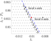 |
Fig. C.1 Two-dimensional interpolation at the red point dwelling inside the non-uniform grid 𝒢3 in Fig. B.3(b). |
A similar formula holds for ∂f /∂I2.
The procedure of the two-dimensional interpolation of the tabulated function f (I1, I2) on a uniform (or Cartesian) grid is standard in textbooks (e.g., Press et al. 1992). The general idea is to break the multi-dimensional interpolation into several mono-dimensional interpolations as illustrated in Fig. C.1. The algorithm is summarized as follows (Morbidelli 1993)
- (1)
Construct a local coordinate system centered at the target point (It1, I2t) (marked as red pentagram in Fig. C.1): the local x-axis is parallel to the axis I1; the local s-axis is generated with an angle θ with respect to the local x-axis. Usually, we choose θ = π/2 and adjust θ in certain cases.
- (2)
Determine the intersection points (xk ,yk) with k = −k_,…, −1,1, …k+ (marked as blue dots in Fig. C.1) of the local y-axis with each horizontal line I2 = I2,j (dashed line in Fig. C.1) where I2,j· is the second coordinate in 𝒢3. The index k is numbered such that the origin is (x0, yo) = (I1t, I2t), and the intersection points above (below) the local y-axis are numbered by 1,2,… (−1, −2,…). Assuming
 , we have
 (C.2)
(C.2)We preserve only those intersection points inside the grid, namely
 . Denote by P = k+ + k− the total number of the intersection points. Obviously, P is a function of θ11.
 - (3)
Conduct P mono-dimensional interpolations using the tabulated values
 on the horizontal dashed lines to find the value f (xk , yk). Then, conduct another mono-dimensional interpolation using the tabulated values {f (sk) |− k−≤ k ≤ k+} with
  along the s-axis to find f (0) which is the value of the function at the target point (I1t, I2t).
For the mono-dimensional interpolation, various interpolation methods are available such as ordinary polynomial interpolation (Conte & de Boor 1980), piecewise polynomial interpolation (such as spline function, see Atkinson 1989, for example). In this paper, we use mainly the simplest ordinary polynomial interpolation. That is, the Lagrange polynomial p (x) is used to interpolate a tabulated function y (xi) = yi, i = 0, 1,…, M (Conte & de Boor 1980)
 (C.3)
(C.3)
In our work, we choose M = 3 as recommended by Press et al. (1992). Instead of using directly Eq. (C.3), it is more recommended to use the Newton form of the Lagrange polynomial to save computational cost. For this, we directly use the Fortran subroutine polint provided in Press et al. (1992). Expecting improvement in the normalization result, we tried also the cubic spline interpolation method, but found no substantial improvement.
A last remark is on the interpolation for the normalization in Appendix B.4. We mentioned there that for the normalization procedure, we do not need the partial derivative at arbitrary point but only on the nodes (I1,(i,j) I2,j·) of the grid 𝒢3. To evaluate ∂f/∂I1 using the first of Eq. (C.1), we need to interpolate the function f at two target points (I1,(i,j) + δI1,I2,j) ,(I1,(i,j)−δI1,I2.j), which both dwell on the horizontal line I2 = I2,j. So, we only need to conduct two mono-dimensional interpolations using the tabulated values  to find ∂f/∂I1 at each node. However, evaluating ∂f/∂I2 using the second of Eq. (C.2) still requires two two-dimensional interpolations.
Appendix D Model of diurnal Yarkovsky effect
In this paper, the planar ERTBP model is adopted. Assuming that the spin-axis of the asteroid is always perpendicular to the orbital plane (otherwise the asteroid would have z-component force due to the Yarkovsky effect and the planar assumption breaks), the seasonal Yarkovsky effect is then irrelevant while the diurnal Yarkovsky effect works.
We adopt the classical model of diurnal Yarkovsky effect presented by Vokrouhlický (1998) where analytical formulae of the diurnal Yarkovsky force for a spherical rotating body are derived. These formulae are directly presented as follows. Their details can be found in the reference. In the reference frame centered at the barycenter of the spherical asteroid with X-axis pointing to the Sun, and Y-axis orthogonal to the X-axis, the Yarkovsky force valid at arbitrary eccentricity reads
 (D.1)
(D.1)
where α is the absorption coefficient, θ0 is the angle between the spin axis and the normal vector of the orbital plane, Φ is the radiation pressure parameter dependent on the radial distance r from the Sun, the radius of the asteroid R, the mass density ρ through the following
 (D.2)
(D.2)
Θ is referred to as the thermal parameter given by
 (D.3)
(D.3)
where C is the specific thermal capacity, K is the thermal conductivity, and ω is the angular velocity. The three coefficients κ1,κ2, κ3 are defined by
![$\eqalign{ & {\kappa _1} = {{{a^2} + {b^2} + ac + bd} \over {\sqrt 2 {R^\prime }\left( {{a^2} + {b^2}} \right)}},{\kappa _2} = {{{{(a + c)}^2} + {{(b + d)}^2}} \over {2{R^{\prime 2}}\left( {{a^2} + {b^2}} \right)}} \cr & {\kappa _3} = {{ad - bc} \over {\sqrt 2 {R^\prime }\left( {{a^2} + {b^2}} \right)}} \cr & \left[ {\matrix{ {a = A\left( {\sqrt 2 {R^\prime }} \right),b = B\left( {\sqrt 2 {R^\prime }} \right),c = \tilde C\left( {\sqrt 2 {R^\prime }} \right),d = \tilde D\left( {\sqrt 2 {R^\prime }} \right)} \hfill \cr {{R^\prime } = {R \over {{l_s}}},{l_s} = 0.00505156{\rm{m}}\sqrt {{K \over {{K_{{\rm{rock }}}}}}{{{\rho _{{\rm{rock }}}}} \over \rho }{{{C_{{\rm{rock }}}}} \over C}{{\omega (R = 0.5{\rm{m}})} \over \omega }} } \hfill \cr {A(x) = - (x + 2) - {e^x}((x - 2)\cos x - x\sin x)} \hfill \cr {B(x) = - x - {e^x}(x\cos x + (x - 2)\sin x)} \hfill \cr {\tilde C(x) = 3(x + 2) + {e^x}(3(x - 2)\cos x + x(x - 3)\sin x)} \hfill \cr {\tilde D(x) = x(x + 3) - {e^x}(x(x - 3)\cos x - 3(x - 2)\sin x)} \hfill \cr } } \right]. \cr} $](/articles/aa/full_html/2024/09/aa49770-24/aa49770-24-eq400.png) (D.4)
(D.4)
In the above formula, we have assumed the following characteristic values
 (D.5)
(D.5)
By its definition, the X-axis is opposite to the usually defined radial direction, and the Y-axis is opposite to the usual transverse direction. So, using Gauss’s form of the perturbation equation, we can derive the differential rate of Keplerian elements of the asteroid due to the Yarkovsky force. It is then straightforward to use the variable transformation Eq. (2) to write the Yarkovsky force FY in terms of the resonance chart as follows
 (D.6)
(D.6)
where S = − fx, T = −fY,  ,
,  ,
,  , and f1 and E1 are the true anomaly and the eccentric anomaly of the asteroid m1.
Appendix E Verification of the normalization result: Surface of section and numerical integration of example orbits
As seen from Fig. 1, the validity of the partial normal form  is subject to the validity of the system
  , and the normalization algorithm. We run simulations in this section to show that the dynamics of the truncated system
  as well as that of the partial normal form
  agrees with that of
  .
.
E.1 Surface of section
We first compared the surfaces of section of the two systems  and
and  , which both have two degrees of freedom. The two systems are bridged by the canonical transformation ℒ2, by which P2 = I2 and
  if
if  (see Eq.(B.4)). So for comparison, it is convenient to choose the section
  for the system
  to generate surfaces on the phase plane
  , and the section θ1 = 0 for the system
  to generate surfaces on the phase plane (θ2,I2).
Figure E.1 presents the superimposition of the surfaces of section of  and
and  on the same energy level manifold, namely
  . The energy level is chosen to be the one that contains a stable equilibrium of ν5 resonance predicted by the partial normal form
  , which is located at (J1e, J2e,ψ2e) = (−0.0276259,0.8407434,0). So, we have
  . Then, we determine a set of initial conditions S1 to generate the surfaces of section by first generating a grid on the phase plane (θ2, I2) and solving I1 by the implicit energy equation, namely
 (E.1)
(E.1)
where I2,min, I2,max are manually given while keeping in mind that the initial conditions in S1 as well as the flows determined by them must dwell inside the working domain 𝒢3 (Fig. B.3(b)). Though we could repeat the above procedure to find a set of initial conditions for  , instead we choose to derive from the set S1 a set S2
 (E.2)
(E.2)
to generate surfaces for  . Although at the risk of not being strict, since the initial conditions in S2 may not dwell exactly on the energy level manifold
  , this tests whether the truncation of the Fourier series
  has been done properly.
In Fig. 4, we mark the level curve I1 = −0.0176259, which is close to the level curves of J1 = J1,e since ℒ3 is near-identity. The level curve I1 = −0.0176259 intersects both the red and the blue curves of stable ν5 centers at ψ2 = 0 and ψ2 = π. So, we could expect two stable centers at  and
and  , respectively on the surfaces of section. This is exactly the case shown in Fig. E.1, which indicates the correctness of our normalization algorithm. Moreover, the phase space structures of the two systems
  and
and  revealed by the surfaces are clearly in qualitative agreement. This indicates the validity of the system
  . A last remark is that in Fig. E.1, we do not observe neither a stable center at
  with a large value of
  , nor a stable center at
  with a small value of
  . This supports our previous argument in Sect. 3.1.2 that the resonance structures that change as the normalization order increases are not real and do not reflect the real dynamics of the original system.
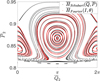 |
Fig. E.1 Superimposition of two surfaces of section obtained by |


E.2 Numerical integration of example orbit
In the above, we show that the phase space structures of the systems  ,
,  and
and  are in qualitative agreement. In this section we carry quantitative comparisons of these systems by numerical integration of example orbits. The initial conditions used for numerical integration of different systems correspond to the same flow bridged by the transformations ℒ2, ℒ3. In fact, to test the validity of the perturbation scheme, we adopt the initial conditions (J2e, ψ2e) corresponding to an equilibrium of v5 resonance determined by the system
  . We choose the equilibrium at ψ2e = π with J1 = −0.0179509. Then, choosing ψ1 = 0, we obtain the corresponding initial conditions (I, θ) = ℒ3 ○ (J,ψ) and
  = ℒ2 ○ (I, θ) for the numerical integrations of
  and
and  , respectively.
To directly compare the ephemeris of the three systems is not convenient since it requires knowledge of ℒ2 for an arbitrary value of θ1, which is cumbersome (as mentioned several times in Appendix B.2). Instead, we directly compare the evolution of three systems without consulting ℒ2, ℒ3 in Fig. E.2 using the properties that (1) ,
,  where ρ (t) is a periodic oscillation dependent on θ1 (t); (2) (J, ψ) can be considered as the mean values of (I, θ), which eliminates the quasi-periodic oscillations dependent on ψ1. The first property indicates that if the truncation of Fourier series Eq. (10) to reach the system
  is done properly, we should expect that the evolutions of
  , I2 generally coincides, and
  oscillates around θ2(t)· This is exactly the cases as shown by all four frames in Fig. E.2. The second property indicates if the normalization algorithm is carried out correctly, (I (t), θ (t)) should oscillate around (J (t), ψ (t). Moreover, as the flow of
  is an equilibrium of v5 resonance, we should expect that I1,I2, θ2 exhibit only periodic oscillations but no secular evolutions. This is exactly the case as shown by frames (c) and (d) in Fig. E.2, which indicates the correctness of the normalization algorithm to order four.
Though the above simulations are for specific energy manifold and orbit, the numerical boundary of a validity region for the normalization algorithm can be established. First, the level curve I1 = −0.0176259 can be taken as a boundary on the right-hand side of which the three systems are in qualitative agreement. Second, using the same truncated expansion, the normal form is expected to have similar performance as Fig. E.2 at those points that have similar convergence speed of Fourier expansion as the yellow dot marked in Fig. 4(c). Then, the level curve of σL (see Appendix B) evaluated at the yellow dot presents a validity boundary. At last, the above two boundaries do not consider the width of the stochastic layer enveloping the J2:1 separatrix due to the overlaps of neighboring resonances, for which we may directly consult the results in Fig. 5, that is, the boundary consisting of the leftmost black crosses that have corresponding circles dwelling exactly on them. The three numerical boundaries mentioned above are presented in Fig. B.3(a).
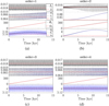 |
Fig. E.2 Comparisons of the numerical integration results of three systems |


Appendix F Analytical treatment of the Type la drift with small eccentricities and small libration amplitude of J2:1 resonance
In the case of the planar circular restricted three body problem (CRTBP) with a small orbital eccentricity of the asteroid, that is i1 = 0, e1 ≪ 1, and e2 = 0, the resonant Hamiltonian for the J2:1 resonance can be reduced to the second fundamental model (abbreviated as SFM, see Lemaître 2010)
 (F.1)
(F.1)
The system is 1-DOF with a parameter δ1. The derivation of the model Eq. (F.1) from the complete Hamiltonian of CRTBP is well developed in literature (Henrard & Lemaitre 1983a), and only briefly described in the following for simplicity. First, develop the disturbing function (namely R in Eq. (A.2)) into a trigonometric series in terms of e1 using the classical elliptic expansion and the Laplace coefficients. Then, average the disturbing function over the mean motions using the following chart (compared to the resonance variables Eq. (2), the following is more suitable for expansion)
 (F.2)
(F.2)
The averaged system is 2-DOF with a parameter p3. Because  ,
,  so that |p1| ≪|p2|, the Hamiltonian is further expanded in terms of p1/p2. Then, apply a variable transformation
  ,
,  and a rescale of the time variable τ = γt. if we choose
  ,γ = −α2η (see Eq. (F.3)), then the transformed Hamiltonian takes exactly the form of the SFM in Eq. (F.1) after discarding negligible terms. The expressions of coefficients mentioned above are12
 (F.3)
(F.3)
Following the argument in Sect. 4.2.1, we calculate the variation of δ1 (equivalently p2) due to the Yarkovsky force. instead of the model in Appendix D, we consider here a simpler model of diurnal Yarkovsky effect
 (F.4)
(F.4)
Following the treatment in Appendix D, in case of (F.4), the Gauss’s form of the perturbation equation gives
 (F.5)
(F.5)
Assuming that e1 ≪ 1 and the variation of a1 is small so that a1 ≈ a1,0 = 3.27 AU, we obtain
 (F.6)
(F.6)
Considering the rescale of the time variable, the parameter  in Eq. (F.1) is slowly varying with
  . To account for the variation of
  , a term
  can be introduced into Eq. (F.1).
Following the perturbation scheme in Sect. 2, the next is to compute the action angle variable of the system Eq. (F.1). As mentioned in Henrard (1993), though it is possible to compute analytically the adiabatic invariant of SFM, the result can be quite involved. So, we take a further simplification by considering small oscillations around the equilibrium. For the analysis of the bifurcation of the equilibrium of the SFM, one may refer to Henrard & Lemaitre (1983b). We carry out a local expansion in the neighborhood of the resonance center located at  through the canonical transformation
  generated by
  . The expansion of the transformed Hamiltonian in terms of q, p truncated to the second degree reads
 (F.7)
(F.7)
where we have assumed a linear variation of λ with a constant rate ϵ′. This is a valid approximation as long as β in Eq. (F.6) is small enough. Fixing λ, the action variable J of Eq. (F.7) is explicitly solved as  . The canonical transformation from (p, q) to the action-angle variable (J, θ) is generated by the generating function S′ = ∫ p (J, q) dq. Considering S′ as a time dependent transformation through λ = λ(t), the transformed Hamiltonian is
 (F.8)
(F.8)
where  . The coordinate transformation generated by S′ is
 (F.9)
(F.9)
We may solve the canonical equation of Eq. (F.7) (see Eq. (9.16) in Boccaletti & Pucacco (1999)) by the following series expansion
 (F.10)
or the Hamiltonian can be developed into a trigonometric series in terms of the small parameter ε′ and normalized. In either way, we should find ℐn in Eq. (F.10) to be periodic so that J, which is the oriented area of the encircled flow (equivalent to J1 in Sect. 4.2.1), is an adiabatic invariant. We then arrive at the same result in Sect. 4.2.1, that is, J1 can be treated as a constant for Type Ia drift.
Now, the effects of Yarkovsky force can be explained using Eq. (F.9). Consider prograde asteroids first. The semi-major axis increases so that β > 0 as told by Eq. (F.4). Then from Eq. (F.5)  . The eccentricity at the equilibrium center also increases because
  where a1 ≈ a1,0. From Eq. (F.9), the J2:1 libration amplitude is proportional to ω(λ)/λ since J can be treated as a constant as argued earlier. For β > 0,
  increases as e1 at the equilibrium increases. Since ∂(ω (λ)/λ)/∂λ < 0, the J2:1 libration amplitude decreases.
We conclude that for prograde asteroids, the eccentricity shows a systematic increase while the J2:1 libration amplitude decreases. For retrograde asteroids, β changes its sign so that the eccentricity shows a systematic decrease while the J2:1 libration amplitude increases.
References
- Atkinson, K. E. 1989, An Introduction to Numerical Analysis (Hoboken: John Wiley & Sons) [Google Scholar]
- Beaugé, C., & Roig, F. 2001, Icarus, 153, 391 [CrossRef] [Google Scholar]
- Boccaletti, D. & Pucacco, G. 1999, Theory of Orbits: Perturbative and Geometrical Methods (Berlin: Springer) [Google Scholar]
- Bottke, W. F., Vokrouhlický, D., Broz, M., Nesvorný, D., & Morbidelli, A. 2001, Science, 294, 1693 [NASA ADS] [CrossRef] [Google Scholar]
- Brož, M., & Vokrouhlický, D. 2008, MNRAS, 390, 715 [CrossRef] [Google Scholar]
- Brož, M., Vokrouhlický, D., Roig, F., et al. 2005, MNRAS, 359, 1437 [CrossRef] [Google Scholar]
- Brož, M., Vokrouhlický, D., Morbidelli, A., Nesvorný, D., & Bottke, W. F. 2011, MNRAS, 414, 2716 [Google Scholar]
- Chrenko, O., Brož, M., Nesvorný, D., Tsiganis, K., & Skoulidou, D. K. 2015, MNRAS, 451, 2399 [NASA ADS] [CrossRef] [Google Scholar]
- Conte, S. D., & de Boor, C. 1980, Elementary Numerical Analysis (New York: McGraw-Hill Book Company) [Google Scholar]
- Dermott, S. F., Jayaraman, S., Xu, Y. L., Gustafson, B. Å. S., & Liou, J. C. 1994, Nature, 369, 719 [CrossRef] [Google Scholar]
- Farinella, P., Vokrouhlický, D., & Hartmann, W. K. 1998, Icarus, 132, 378 [NASA ADS] [CrossRef] [Google Scholar]
- Fenucci, M., Novakovic´, B., Vokrouhlický, D., & Weryk, R. J. 2021, A&A, 647, A61 [NASA ADS] [CrossRef] [EDP Sciences] [Google Scholar]
- Ferraz-Mello, S. 2007, Canonical Perturbation Theories - Degenerate Systems and Resonance (Berlin: Springer), 345 [Google Scholar]
- Ferraz-Mello, S., Michtchenko, T. A., & Roig, F. 1998a, AJ, 116, 1491 [NASA ADS] [CrossRef] [Google Scholar]
- Ferraz-Mello, S., Nesvorny, D., & Michtchenko, T. A. 1998b, ASP Conf. Ser., 149, 65 [NASA ADS] [Google Scholar]
- Ferraz-Mello, S., Beaugé, C., & Michtchenko, T. A. 2003, Celest. Mech. Dyn. Astron., 87, 99 [CrossRef] [Google Scholar]
- Goldreich, P., & Peale, S. 1966, AJ, 71, 425 [NASA ADS] [CrossRef] [Google Scholar]
- Gomes, R. S. 1995, Icarus, 115, 47 [NASA ADS] [CrossRef] [Google Scholar]
- Granvik, M., Morbidelli, A., Jedicke, R., et al. 2018, Icarus, 312, 181 [CrossRef] [Google Scholar]
- Henrard, J. 1990, Celest. Mech. Dyn. Astron., 49, 43 [NASA ADS] [CrossRef] [Google Scholar]
- Henrard, J. 1993, The Adiabatic Invariant in Classical Mechanics, eds. C. K. R. T. Jones, U. Kirchgraber, & H. O. Walther (Berlin, Heidelberg: Springer Berlin Heidelberg), 117 [Google Scholar]
- Henrard, J., & Lemaitre, A. 1983a, Icarus, 55, 482 [NASA ADS] [CrossRef] [Google Scholar]
- Henrard, J., & Lemaitre, A. 1983b, Celest. Mech., 30, 197 [Google Scholar]
- Henrard, J., & Lemaitre, A. 1987, Icarus, 69, 266 [NASA ADS] [CrossRef] [Google Scholar]
- Henrard, J., Watanabe, N., & Moons, M. 1995, Icarus, 115, 336 [NASA ADS] [CrossRef] [Google Scholar]
- Laskar, J. 2003, arXiv e-prints [arXiv:math/0305364] [Google Scholar]
- La Spina, A., Paolicchi, P., Kryszczyn´ska, A., & Pravec, P. 2004, Nature, 428, 400 [NASA ADS] [CrossRef] [Google Scholar]
- Lemaître, A. 2010, in Lecture Notes in Physics, eds. J. Souchay, & R. Dvorak (Berlin: Springer), 790, 1 [CrossRef] [Google Scholar]
- Levison, H. F., & Duncan, M. J. 1994, Icarus, 108, 18 [NASA ADS] [CrossRef] [Google Scholar]
- Liu, X., Hou, X.-Y., Yang, Z.-T., Gan, Q.-B., & Zhang, Y. 2023, ApJ, 950, 50 [NASA ADS] [CrossRef] [Google Scholar]
- Moons, M. 1994, Celest. Mech. Dyn. Astron., 60, 173 [NASA ADS] [CrossRef] [Google Scholar]
- Moons, M., & Morbidelli, A. 1993, Celest. Mech. Dyn. Astron., 57, 99 [NASA ADS] [CrossRef] [Google Scholar]
- Moons, M., Morbidelli, A., & Migliorini, F. 1998, Icarus, 135, 458 [NASA ADS] [CrossRef] [Google Scholar]
- Morbidelli, A. 1993, Celest. Mech. Dyn. Astron., 55, 101 [NASA ADS] [CrossRef] [Google Scholar]
- Morbidelli, A. 2002, Modern Celestial Mechanics: Aspects of Solar System Dynamics (Boca Raton: CRC Press) [Google Scholar]
- Morbidelli, A., & Moons, M. 1993, Icarus, 102, 316 [NASA ADS] [CrossRef] [Google Scholar]
- Morbidelli, A., & Vokrouhlický, D. 2003, Icarus, 163, 120 [NASA ADS] [CrossRef] [Google Scholar]
- Nesvorný, D., Ferraz-Mello, S., Holman, M., & Morbidelli, A. 2002, in Asteroids III (Tucson: University of Arizona Press), 379 [CrossRef] [Google Scholar]
- Peterson, C. 1976, Icarus, 29, 91 [NASA ADS] [CrossRef] [Google Scholar]
- Press, W. H., Teukolsky, S. A., Vetterling, W. T., & Flannery, B. P. 1992, Numerical Recipes in FORTRAN. The Art of Scientific Computing (Cambridge: Cambridge University Press) [Google Scholar]
- Roig, F., Nesvorný, D., & Ferraz-Mello, S. 2002, MNRAS, 335, 417 [NASA ADS] [CrossRef] [Google Scholar]
- Vokrouhlický, D. 1998, A&A, 335, 1093 [Google Scholar]
- Vokrouhlický, D., & Farinella, P. 1998, AJ, 116, 2032 [CrossRef] [Google Scholar]
We find that a non-zero value ɡ5 = 4.2575″ yr−1 (a value adopted in Morbidelli & Moons 1993) does not influence the conclusion in this paper. The advantage of the choice ɡ5 = 0 is that the results can be directly verified using the N-body simulation SWIFT package as in Fig. 5.
Generally, we should have  . However, this is not the case (or N must be taken very large to allow for a small ɛ) if
  corresponds to the orbital configuration where the high-eccentricity asteroid orbit intersects the Jupiter’s orbit. In this case, the collision singularity |r1 − r2| = 0 affects the accuracy of the Riemann summation. This problem is inherited by ε2 in Eq. (8).
This can be understood as the characteristic timescale of the v5 resonance generally being much longer than that of the J2:1 resonance. We note that this degeneracy obviously breaks in the chaotic region where low-order secondary resonances between θ1 and θ2 occur; see Sect. 3.1.1.
It is important to note that the setting ψ1 = 0 is necessary because in this case we always have θ1 = 0 if ψ2 = 0, π under the mapping ℒ3,n (note that ℒ3,0 = ℒ3,1 is adopted). Then, for θ1 = 0, we always have  and
and  under the mapping ℒ2. Since
  is just the section to find the libration boundaries of
  , we could superimpose the result directly on Fig. 2. We also note that though the Lie mapping ℒ3,n in Eq. (21) is a near-identity transformation, its effect is non-negligible in some cases (particularly for equilibriums with ψ2c = π). However, the differences between ℒ3,1 and ℒ3,n≥2 are of higher orders. Thus, in some cases, it is convenient to directly use ℒ3,1 for higher order partial norm forms.
The dots are distributed in a small region  and
and  so that they basically overlap under the scale in Fig. 4 and thus appear like a single dot.
The settings of physical parameters for the Yarkovsky effects are the same as those in Sect. 4.1 except that the radius is chosen as R = 50 m.
We note that in our study, three regions are studied separately: region-α 0.001 < e1 < 0.2 for the secondary resonances (see Sect. 3.1.1 ); region-b 0.2 ≤ e1 ≤ 0.9, which excludes the region-α and covers the dynamical structures of v5 resonance inside the J2:1 resonance; and region-c 0.001 ≤ e1 ≤ 0.54, which focuses on the part of v5 resonance close to the J2:1 libration boundary. The analysis of region-c is treated in this appendix as an example.
There are cases when P is too small for θ = π/2 or when the target point is close to the ends of the local y-axis, which is not usually recommended (Conte & de Boor 1980). In this case, we adjust the value of θ in the obvious way.
A somewhat non-strict point here is that the coefficients are functions of p2. When considering p2 a slowly varying parameter, which is the case later, the above variable transformations are in fact time dependent and thus not canonical. However, considering that p2 very slowly, the discrepancy should be small and does not influence the analytical treatment here.
All Figures
|
Fig. 1 Schematic procedures of the perturbative treatments for the Yarkovsky-driven drifts in the J2:1 commensurability under the model of planar ERTBP. |
| In the text | |
|
Fig. 2 Resonance structures (equilibriums and libration width) of the integrable approximation |
| In the text | |
|
Fig. 3 Phase portraits of the integrable approximation |
| In the text | |
|
Fig. 4 Locations of v¡ resonance centers and the corresponding boundaries of the libration domain of the partial normal form |
| In the text | |
|
Fig. 5 Pseudo-proper elements (dots) of orbits inside the J2:1 commen-surability obtained by the SWIFT package. The black crosses mark their initial conditions with 𝑔1 – 𝑔2 ≈ 0 (𝑔1 – 𝑔2 = π) in the left (right) frame. The section Q2 ≈ 0 (Q2 ≈ π) in Eq. (23) is used to record the pseudo-proper elements of each orbit in frame a (frame b). The colored (gray) dots mark the pseudo-proper elements of orbits trapped (not trapped) in the v5 libration domain. |
| In the text | |
|
Fig. 6 Drifts of pseudo-proper elements of orbits inside the J2:1 commensurability due to the diurnal Yarkovsky effect. The initial conditions are the same as those in Fig. 5 while the Yarkovsky effect is included in the force model (see the text for physical parameters related to the Yarkovsky effect). As in Fig. 5, the section Q2 ≈ 0 (Q2 ≈ π) in Eq. (23) is used to record the pseudo-proper elements of each orbit in frame a (frame b). The integration time is 2 Myr. The ν5 resonance structures are taken from Fig. 4. The gray curves are the level curves of I1 that the ν5 libration approximately follows. Compared with Fig. 5, the pseudo-proper elements show obvious systematic drifts. The light yellow curves in frame a mark the pseudo-proper elements obtained using partial normal form H2* perturbed by |
| In the text | |
|
Fig. 7 Trajectories on the (e 1,ɡ1 − ɡ2) plane for example orbits of different types of drift identified in Fig. 6. Frame a presents two orbits of Type Ia marked as gray dots with black edges in the left frame of Fig. 6; Frame b presents two orbits of Type IIa dwelling in the libration domain of Ψ2 = 0 (Ψ2 = π) at |
| In the text | |
|
Fig. 8 Strength-normalized vector field υc/||υc|| on the pseudo-proper a1 − e1 plane for Type I drifts. The colored circles are footprints of Type I ∗ drifts obtained by numerical integration of the partial normal form |
| In the text | |
|
Fig. 9 Contour map of the eccentricity excitation time TIa (e1,i, eı,f) for Type la drift in the J2:1 commensurability. The unit of TIa (e1,i, e 1,f) is Myr with e1,i = 0.2 and e1,f = aJ/aJ2:1 − 1 ≈ 0.59. The diameter D of the asteroid is fixed as 35 m, and the spin period is fixed as 600 s. |
| In the text | |
|
Fig. 10 Strength-normalized vector field υl/||υl|| in the three libration domains of v5 resonance on the pseudo-proper a1 − e1 plane. The colored circles are footprints of Type IIa drifts obtained by numerical integration of the partial normal form |
| In the text | |
|
Fig. 11 Evolution trajectories of four example orbits to show the evolution paths of retrograde asteroids inside the J2:1 resonance. |
| In the text | |
|
Fig. B.1 Left frame: Grid 𝒢1 marked by black crosses, which is the work domain for the integrable approximation |
| In the text | |
|
Fig. B.2 Two typical phase portraits of the integrable approximations |
| In the text | |
|
Fig. B.3 Frame (a): Projection of the grid 𝒢2 onto the |
| In the text | |
|
Fig. B.4 NAFF results of the sampling signal of |
| In the text | |
|
Fig. C.1 Two-dimensional interpolation at the red point dwelling inside the non-uniform grid 𝒢3 in Fig. B.3(b). |
| In the text | |
|
Fig. E.1 Superimposition of two surfaces of section obtained by |
| In the text | |
|
Fig. E.2 Comparisons of the numerical integration results of three systems |
| In the text | |
Current usage metrics show cumulative count of Article Views (full-text article views including HTML views, PDF and ePub downloads, according to the available data) and Abstracts Views on Vision4Press platform.
Data correspond to usage on the plateform after 2015. The current usage metrics is available 48-96 hours after online publication and is updated daily on week days.
Initial download of the metrics may take a while.