© A. T. Sutinjo et al. 2022

1 Introduction

System equivalent flux density (SEFD) is an important figure of merit of a radio telescope. Our previous work in Sutinjo et al. (2021, Paper I, dual-polarized antennas). and the extensions thereof in Sutinjo et al. (2022a, Paper II, tripole/multipole antennas) and Sutinjo et al. (2022b, Paper III, phased array) showed the derivation and validation of SEFD of Stokes I for a polarimetric interferometer. This paper expands the formula to all other Stokes parameters, Q, U, and V. Recent discoveries in polarized astrophysical radio transients highlight the importance of knowing the telescope sensitivity for all four Stokes parameters over a wide field of view. A detailed review of the scientific motivation and application of this work is given in Sect. 4.

The expressions we derive here are valid for dual-polarized antennas up to multipole antennas. The dual-polarized antenna systems are typical of a ground-based polarimetric interferometer, whereas tripole antennas are being proposed for a spaceborne intereferometer (2018, Chen et al. 2021; Huang et al. 2018; Bentum et al. 2020). Therefore, to illustrate this generality, we begin with a tripole antenna system as an example. The extension to a multipole system is straightforward; the simplification to the dual-polarized antenna system will be discussed in Sect. 2.3.

The voltages measured by the tripole antenna system 1 in response to the target electric field (|_t) are (as per Sect. 1 of Paper II): $$\begin{array}{lll}{\text{v}}_1{|}_t\hfill & =\hfill & J_1{\text{e}}_t,\hfill \\ \left[\begin{array}{c}{V}_{X1{|}_t}\\ V_{Y1{|}_t}\\ V_{Z1{|}_t}\end{array}\right]\hfill & =\hfill & \left[\begin{array}{c}{l}_{X1\theta }{l}_{X1\varphi }\\ l_{Y1\theta }{l}_{Y1\varphi }\\ l_{Z1\theta }{l}_{Z1\varphi }\end{array}\right]\left[\begin{array}{c}{E}_{t\theta }\\ E_{t\varphi }\end{array}\right],\hfill \end{array}$$(1)

where J₁ is the Jones matrix of system 1, with entries which represent the antenna effective lengths, in units of m (see Paper I); E_tθ, E_t∅ are the components of the incident electric field vector, in units of Vm⁻¹. The voltages are correlated, resulting in the outer product $${\text{v}}_1{\text{v}}_2^H{|}_t=J_1{\text{e}}_t{\text{e}}_t^H{J}_2^H,$$(2)

where J₂ is the Jones matrix of system 2, and superscript “H” denotes the conjugate transpose.

The quantities of interest are the linear combinations of the entries of $e_t{e}_t^H$ in Eq. (2). The expected value is: $$\begin{array}{ll}\langle e_t{e}_t^H\rangle \hfill & =\left[\begin{array}{cc}{}_{\langle E_{t\theta }^{*}{E}_{t\varphi }\rangle }^{\langle {\left|E_{t\theta }\right|}^2\rangle }& {}_{\langle {\left|E_{t\theta }\right|}^2\rangle }^{\langle E_{t\theta }{E}_{t\varphi }^{*}\rangle }\end{array}\right]\hfill \\ \hfill & =\frac{1}{2}\left[\begin{array}{cc}{}_{U+jV}^{I+Q}& {}_{I-Q}^{U-jV}\end{array}\right],\hfill \end{array}$$(3)

as discussed in Paper I. Equation (3) suggests that the corresponding random variables from which the Stokes parameters are inferred (we drop the subscript “t” for brevity): $$\begin{array}{lll}\tilde{I}\hfill & =\hfill & {\left({\tilde{\text{e}}\tilde{\text{e}}}^H\right)}_{1,1}+{\left({\tilde{\text{e}}\tilde{\text{e}}}^H\right)}_{2,2},\hfill \\ \tilde{Q}\hfill & =\hfill & {\left({\tilde{\text{e}}\tilde{\text{e}}}^H\right)}_{1,1}+{\left({\tilde{\text{e}}\tilde{\text{e}}}^H\right)}_{2,2},\hfill \\ \tilde{U}\hfill & =\hfill & {\left({\tilde{\text{e}}\tilde{\text{e}}}^H\right)}_{1,2}+{\left({\tilde{\text{e}}\tilde{\text{e}}}^H\right)}_{2,1},\hfill \\ \tilde{V}\hfill & =\hfill & j\left[{\left({\tilde{\text{e}}\tilde{\text{e}}}^H\right)}_{1,2}-{\left({\tilde{\text{e}}\tilde{\text{e}}}^H\right)}_{2,1}\right].\hfill \end{array}$$(4)

The SEFD expressions are proportional to the standard deviations of Eq. (4). In Sect. 2, we discuss how they can be obtained.

2 Method: SEFD Derivation

2.1 Expressing Noisy Estimates using Matrix Trace

To obtain $\tilde{e}{\tilde{e}}^H$ from $v_1{v}_2^H$, we need to remove the influence of the Jones matrices. This is possible by forming the left inverse of the Jones matrix, L = (J^HJ)⁻¹ J^H (see Sect. 2 of Paper II). We note that for a dual-polarized system, the left inverse is identical to the matrix inverse. Of course, for the left inverse to exist, the columns of the Jones matrices must be linearly independent, which is not difficult to build into the antenna design.

Using the left inverse, the result is an estimate (see Sect. 2 of Paper II): $$\begin{array}{ll}\tilde{\text{e}}\tilde{\text{e}}\hfill & ={\left(J_1^H{J}_1\right)}^{-1}{J}_1^H{\text{v}}_1{\text{v}}_2^H{J}_2{\left(J_2^H{J}_2\right)}^{-H}\hfill \\ \hfill & =L_1{\text{v}}_1{\text{v}}_2^H{L}_2^H.\hfill \end{array}$$(5)

To obtain the noisy estimates of the Stokes parameters in Eq. (4), we use the matrix trace operation, tr() on Eq. (5). As an example, we start with $\tilde{I}$. $$\tilde{I}=\text{tr\hspace{0.17em}}\left({\tilde{\text{e}}\tilde{\text{e}}}^H\right)=\text{tr\hspace{0.17em}}\left(L_1{\text{v}}_1{\text{v}}_2^H{L}_2^H\right).$$(6)

Applying the trace property of matrix product¹, tr(AB) = tr(BA) which is valid for A (m × n) and B (n × m), successively to Eq. (6), leads to: $$\begin{array}{ll}\tilde{I}\hfill & =\text{tr\hspace{0.17em}}\left({\text{v}}_1{\text{v}}_2^{\text{H}}{L}_2^{\text{H}}{L}_1\right)=\text{tr\hspace{0.17em}}\left({\text{v}}_2^H{L}_2^H{L}_1{\text{v}}_1\right)\hfill \\ \hfill & ={\text{v}}_2^H{L}_2^H{L}_1{\text{v}}_1.\hfill \end{array}$$(7)

The last equality in Eq. (7) comes from the fact that $v_2^H{L}_2^H{L}_1{v}_1$ produces a single number such that the trace operator is redundant. Similarly, for $\tilde{Q}$: $$\begin{array}{ll}\widehat{Q}\hfill & =\text{tr\hspace{0.17em}}\left(P_Q{\tilde{\text{e}}\tilde{\text{e}}}^H\right)=\text{tr\hspace{0.17em}}\left(P_Q{L}_1{\text{v}}_1{\text{v}}_2^H{L}_2^H\right)\hfill \\ \hfill & ={\text{v}}_2^H{L}_2^H{P}_Q{L}_1{\text{v}}_1,\hfill \end{array}$$(8)

where $$P_Q=\left[\begin{array}{cc}1& 0\\ 0& -1\end{array}\right].$$(9)

Similarly, $$\tilde{U}={\text{v}}_2^H{L}_2^H{P}_U{L}_1{\text{v}}_1,$$(10) $$\tilde{V}={\text{v}}_2^H{L}_2^H{P}_V{L}_1{\text{v}}_1,$$(11)

where $$P_U=\left[\begin{array}{cc}0& 1\\ 1& 0\end{array}\right],$$(12) $$P_V=j\left[\begin{array}{cc}0& -1\\ 1& 0\end{array}\right].$$(13)

We now see that $\tilde{I}$ in Eq. (7) is a special case in which P_I = I, that is the identity matrix. For brevity we will refer to $L_2^H{P}_S{L}_1=M_S$ where the subscript “S ” denotes the Stokes parameter of interest: I, Q, U, or V.

2.2 SEFD Formula

Following the same derivation steps as (see Sects. 2 and 3, Appendix of Paper II), we can show that: $$\text{=\hspace{0.17em}}{\text{SEFD}}_S=\frac{4k}{{\eta }_0}\sqrt{t_{\text{sysR1}}^T\left(M_S\circ M_S^{*}\right)t_{{\text{sysR}}_2},}$$(14)

where “o” refers to the element-by-element product, and superscript “*” denotes complex conjugation such that $M_S\circ M_S^{*}$ produces the magnitude squared of each entry of M_S ; $$M_{S=}{}_{I,Q,U,V}=L_2^H{P}_{S=I,Q,U,V}{L}_1,$$(15)

where P_I, P_q, P_U, P_V are shown in Sect 2.1 and $${\text{t}}_{s\text{ysR1}}=\left[\begin{array}{c}{T}_{sysX1}{R}_{\text{ant}X1}\\ T_{sysY1}{R}_{\text{antY}1}\\ T_{sysZ1}{R}_{\text{ant}Z1}\end{array}\right],$$(16)

and similarly for t_sysR2 (with entries that pertain to T_sys’s and R_ant’s of system 2).

2.3 Special Case: Dual-Polarized Antennas with an Identical Antenna Design

We consider a typical case of X and Y dual-polarized antennas which are common in ground-based radio astronomy. In this case, the last row in Eq. (1) is removed. Furthermore, an identical antenna design implies an identical Jones matrix, J₁ = J₂ = J_dual, where $$J_{\text{dual}}=\left[\begin{array}{ll}{l}_{X\theta }\hfill & l_{X\varphi }\hfill \\ l_{Y\theta }\hfill & l_{Y\varphi }\hfill \end{array}\right].$$(17)

The left inverse becomes the inverse, $L=J_{\text{dual}}^{-1}$ such that $$M_{S:dual}=J_{\text{dual}}^{-H}{P}_S{J}_{\text{dual}}^{-1}.$$(18)

As a result $${\text{SEFD}}_{S:dual}=\frac{4k}{{\eta }_0}\sqrt{t_{\text{sysR1}}^T\left(M_{S:\text{dual}}\circ M_{S:\text{dual}}^{*}\right)t_{\text{sysR2}}.}$$(19)

It can be shown that (see Sect 2.5 of Paper III): $$M_{I:dual}=\frac{1}{{\Vert l_X-p\Vert }^2{\Vert I_Y\Vert }^2}\left[\begin{array}{ll}{\Vert I_Y\Vert }^2\hfill & -I_X^H{I}_Y\hfill \\ -I_X^H{I}_Y\hfill & {\Vert I_X\Vert }^2\hfill \end{array}\right],$$(20)

where ‖.‖ operator refers to the length of the vector in question, such that‖I_X‖ and ‖I_Y‖ are the lengths of the row vectors of J_dual, I_X = [l_Xθ, l_X∅]^T, similarly with I_Y. The denominator in the right hand side of Eq. (20) is the absolute value squared of the determinant of the Jones matrix. $${\left|D\right|}^2={\left|l_{X\theta }{l}_{Y\theta }-l_{X\varphi }{l}_{Y\theta }\right|}^2={\Vert l_X-p\Vert }^2{\Vert l_Y\Vert }^2,$$(21)

where p is the projection vector of I_X onto I_Y. By expanding the matrix algebra, we find for Stokes Q, $${\left|D\right|}^2{M}_Q=\left[\begin{array}{ll}{\left|l_{Y\varphi }\right|}^2-{\left|l_{Y\varphi }\right|}^2\hfill & -l_{Y\varphi }^{*}{l}_{X\varphi }+l_{Y\varphi }^{*}{l}_{X\theta }\hfill \\ l_{X\varphi }^{*}{l}_{Y\varphi }+l_{X\theta }^{*}{l}_{Y\theta }\hfill & {\left|l_{X\varphi }\right|}^2-{\left|l_{X\theta }\right|}^2\hfill \end{array}\right],$$(22)

where we dropped the .:_dual subscript for brevity. For Stokes U: $${\left|D\right|}^2{M}_U=\left[\begin{array}{ll}-2\Re \left(l_{X\varphi }^{*}{l}_{Y\theta }\right)\hfill & -l_{Y\varphi }^{*}{l}_{X\theta }+l_{Y\theta }^{*}{l}_{X\varphi }\hfill \\ l_{X\varphi }^{*}{l}_{Y\theta }+l_{X\theta }^{*}{l}_{Y\varphi }\hfill & -2\Re \left(l_{X\varphi }^{*}{l}_{Y\theta }\right)\hfill \end{array}\right].$$(23)

Finally, for Stokes V, $${\left|D\right|}^2{M}_V=\left[\begin{array}{ll}-2j\mathfrak{J}\left(l_{X\varphi }^{*}{l}_{Y\theta }\right)\hfill & -l_{Y\varphi }^{*}{l}_{X\theta }+l_{Y\theta }^{*}{l}_{X\varphi }\hfill \\ -l_{X\varphi }^{*}{l}_{Y\theta }+l_{X\theta }^{*}{l}_{Y\varphi }\hfill & -2j\mathfrak{J}\left(l_{X\varphi }^{*}{l}_{X\theta }\right)\hfill \end{array}\right].$$(24)

Example results for a dual polarized dipoles and the Murchison Widefield Array (MWA) are shown in the next section.

3 Results

3.1 X-Y Short Dipoles

We begin by considering simple X-Y short dipoles. In this case, the Jones matrix is real: $$\begin{array}{ll}J\hfill & =\left[\begin{array}{c}\cos \theta \cos \varphi -\sin \varphi \\ \cos \theta \sin \varphi \cos \varphi \end{array}\right]\hfill \\ \hfill & =\left[\begin{array}{c}\cos \varphi -sin\varphi \\ \sin \varphi -\cos \varphi \end{array}\right]\left[\begin{array}{ll}\cos \theta \hfill & 0\hfill \\ 0\hfill & 1\hfill \end{array}\right]=R\Sigma .\hfill \end{array}$$(25)

In Eq. (25), the antenna length in units of meter could be included by pre-multiplying the matrix with a scalar l. The decomposition in Eq. (25) was discussed in Paper I, where R is an orthogonal (rotation) matrix (R^TR = RR^T = I, the identity matrix) and Σ is a diagonal matrix that contains the singular values. As a result, we can write the following: J⁻¹ = (RΣ)⁻¹ = Σ⁻¹R⁻¹ = Σ⁻¹R^T ; J^−H = RΣ⁻¹; and $$\begin{array}{c}{\text{Σ}}^{-1}{R}^{-1}={\text{Σ}}^{-1}{R}^T;J^{-H}=R{\text{Σ}}^{-1};\text{\hspace{0.17em}and}\\ M_S=J^{-H}{P}_S{J}^{-1}=R{\text{Σ}}^{-1}{P}_S{\text{Σ}}^{-1}{R}^T.\end{array}$$(26)

Assuming identical antennas (R_antX = R_antY = R_ant) and the same system temperatures for X and Y (T_sysX = T_sysY = T_sys), it can be shown that Eq. (18) becomes (see Paper II): $$\begin{array}{ll}{\text{SEFD}}_S\hfill & =\frac{4k{R}_{\text{ant}}{T}_{\text{sys}}}{{\eta }_0}\sqrt{\left[1,1\right]\left(M_S\circ M_S^H\right){\left[1,1\right]}^T}\hfill \\ \hfill & =\frac{4k{R}_{\text{ant}}{T}_{\text{sys}}}{{\eta }_0}\sqrt{\text{tr\hspace{0.17em}}\left(M_S{M}_S^H\right)}.\hfill \end{array}$$(27)

Using Eq. (26): $$\begin{array}{ll}{M}_S{M}_S^H\hfill & =R{\text{Σ}}^{-1}{P}_S{\text{Σ}}^{-1}{R}^{T}R{\text{Σ}}^{-1}{P}_S^H{\text{Σ}}^{-1}{R}^T\hfill \\ \hfill & =R{\text{Σ}}^{-1}{P}_S{\text{Σ}}^{-2}{P}_S^H{\text{Σ}}^{-1}{R}^T.\hfill \end{array}$$(28)

The inverse of Σ in Eq. (25) is easily done by inverting the diagonal entries. Using the relevant P_S matrix shown in Sect 2.1, we can show that $$\begin{array}{ll}{M}_{\text{I}}{M}_{\text{I}}^{\text{H}}=M_Q{M}_Q^H\hfill & =R{\text{Σ}}^{-4}{R}^T\hfill \\ \hfill & =R\left[\begin{array}{ll}{\cos }^{-4}\theta \hfill & 0\hfill \\ 0\hfill & 1\hfill \end{array}\right]R^T.\hfill \end{array}$$(29)

Since R is orthogonal, Eq. (29) is an eigendecomposition of $M_I{M}_I^H$ and $M_Q{M}_Q^H$ where Σ⁻⁴ is the eigenvalue matrix. As a result, the trace of that matrix is simply the sum of the eigenvalues (Strang 2016, see Chap. 6); the same result could also have been obtained by applying the trace of matrix product property shown in Sect 2.1, tr(RΣ⁻⁴R^T) = tr(Σ⁻⁴R^TR) = tr(Σ⁻⁴). $${\text{SEFD}}_I={\text{SEFD}}_Q=\frac{4\pi R_{\text{ant}}{T}_{\text{sys}}}{{\eta }_0}\sqrt{{\cos }^{-4}\theta +1}.$$(30)

The SEFD_I dependence as a function θ is the same as that identified in Sect. 4 of Paper I. The effect of the metallic ground screen and/or actual antenna length can be easily added, if desired, as a multiplicative factor, l(θ)⁻², in units of m⁻² in the SEFD expression.

Similarly, by using Eq. (28) and substituting the relevant P_S, we can show that: $$M_U{M}_U^H=M_V{M}_V^H=R\left(I{\text{cos}}^{-2}\theta \right)R^T,$$(31)

such that $${\text{SEFD}}_U={\text{SEFD}}_V=\frac{4\pi R_{\text{ant}}{T}_{\text{sys}}}{{\eta }_0}\frac{\sqrt{2}}{\cos \theta }.$$(32)

Therefore, for the orthogonal short dipole system, the SEFD is only dependent on θ, the zenith angle. This was validated by numerical calculations based on Eq. (19) and the Jones matrix as originally presented in Eq. (25). Figure 1 shows the SEFD I, Q, U, and V normalized to the minimum of SEFD_I (at θ = 0°) as a function of zenith angle. It clearly shows that SEFD_U and SEFD_V rise more slowly than SEFD_I and SEFD_q with increasing θ as expected from Eqs. (30) and (32).

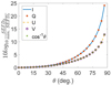Fig. 1 SEFDI,Q,U,V/min. SEFDI in decibel (dB) as a function of zenith angle, θ.

3.2 MWA Telescope Pointing at ZA = 46.1°, Az = 80.5°

The same observational data at 154.88 MHz as reported in Paper III was reprocessed and used to compute SEFD_Q,U,V using the same methods as described in Paper III. For clarity, the observation took place on the 26th December 2014 at 16:05:42 hr UTC time with the MWA telescope (Tingay et al. 2013) pointing at grid point 114 (ZA = 46.1°, Az = 80.5°). All observational images have a size of 4096 × 4096 pixels and were smoothed in Matlab with a Gaussian filter of size 201 × 201 to reduce the effects of noise.

The absolute values between simulated and observed SEFD_I were verified in Paper III; therefore, to validate Eq. (19), it is sufficient to show that the predicted ratio of SEFD_U/SEFD_I, SEFD_V/SEFD_I, and SEFD_Q/SEFD_I match the observation data. Figure 2a shows the predicted SEFD_U /SEFD_I calculated using Eq. (19) based on the simulated MWA array, while Fig. 2b shows the observed SEFD_U /SEFD_I. The solid contour lines seen in Figs. 2, 3, and 4 represent a change in level of 0.1. For ease of comparison, the simulated (black) contour lines shown in Fig. 2a were transferred to Fig. 2b and are shown as white contour lines. The black contour lines in Fig. 2b represent the contours of the observation data after smoothing. Therefore, the comparison we suggest here is between the white and black contour lines in Fig. 2b. We observe that the simulated contours predict the trends of the observed contours very well. Furthermore, the simulated contours are within a few percent of the observation.

We repeated this process in Figs. 3 and 4. Figures 3b and 4b show the observed SEFD_V/SEFD_I and SEFD_q/SEFD_I respectively. The agreement between the simulation and observation in Fig. 3b is very similar to that in Fig. 2b. We calculated average percentage differences between the simulation and observation over the entire images of SEFD_U/SEFD_I and SEFD_V/SEFD_I of approximately 3.6 and 3.5%, respectively. Notwithstanding the excellent overall agreement over the images, we see a small systematic offset of approximately 3.5% between the observed and simulated contour lines in Figs. 2b and 3b. The exact reason for this is not fully understood. However, we note that agreement of the SEFD_U/SEFD_I and SEFD_V/SEFD_I is similar to the level of agreement within a few percent between simulation and observation in our previous work (Sutinjo et al. 2021, Sutinjo et al. 2022b) and is expected. A further contributing factor to the offset could be the presence of a non-functional dipole in an MWA tile due to a damaged low noise amplifier. Preliminary simulations of an MWA tile with a non-functional dipole suggest the systematic offset of a few percent could vanish or increase depending on the location of the broken dipole. However, the inclusion of models that include random non-functioning dipoles throughout the entire MWA telescope requires extensive further study which may be addressed in future work. In Fig. 4a, we note that while contours lines of the simulated values are included, they are not visible since they only start to change from 1 to 0.9 at the top left and bottom right corners.

We see an excellent agreement between the simulated and observed SEFD_q/SEFD_I, with an average percentage difference of 1.8% between the observed and simulated results. The near equality between SEFD_I and SEFD_Q seen in the image is consistent with that suggested by the idealized calculation in Sect. 3.1. The noticeable object in the center of Figs. 2b, 3b, and 4b is the calibrator source Hydra-A which was the main target of the analyzed observation. This is an artifact of the difference imaging and is not relevant to SEFD calculation.

The simplified calculation in Sect. 3.1 suggests that SEFD_U/SEFD_I and SEFD_V/SEFD_I are less than or equal to unity for X-Y dipoles. This is consistent with Figs. 2b and 3b. In addition, it is also made evident in the comparison of the contour shapes in Figs. 2b and 3b that SEFD_U and SEFD_V are nearly equal, which is again consistent with the findings reported in Sect. 3.1. These agreements are expected because the MWA antennas at this observing frequency can be approximated as X-Y short dipoles.

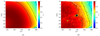Fig. 2 Side-by-side comparison of the ratio of the simulated and observed SEFDU/SEFDI at gridpoint 114. (a) Simulated image of SEFDU/SEFDI with the corresponding contour levels. (b) Observed SEFDU/SEFDI with the corresponding contour levels (black curves) and the contour levels of the simulated values (white curves). The observed image has a size of 4096 × 4096 pixels and was smoothed using a Gaussian filter of size 201 × 201 to smooth the noisy image.

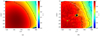Fig. 3 Side-by-side comparison of the ratio of the simulated and observed SEFDV/SEFDI at gridpoint 114. (a) Simulated image of SEFDV/SEFDI with the corresponding contours levels (black curves). (b) Observed SEFDV/SEFDI with the corresponding contours levels (black curves) and the contour levels of the simulated values (white curves). The observed image has a size of 4096 × 4096 pixels and was smoothed using a Gaussian filter of size 201 × 201 to smooth the noisy image.

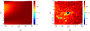Fig. 4 Side-by-side comparison of the ratio of the simulated and observed SEFDq/SEFDI at gridpoint 114. (a) Simulated image of SEFDq/SEFDI with the corresponding contours levels (black curves). (b) Observed SEFDq/SEFDI with the corresponding contours levels (black curves) and the contour levels of the simulated values (white curves). The observed image has a size of 4096 × 4096 pixels and was smoothed using a Gaussian filter of size 201 × 201 to smooth the noisy image.

4 Scientific Applications

Although the majority of radio sources are unpolarized, some astrophysical objects of transient nature, such as pulsars, fast radio bursts (FRBs), or M dwarf stars, exhibit large degree of polarization. For example, Lenc et al. (2018) analyzed MWA data at 169–200 MHz band and demonstrated detection of 33 pulsars in Stokes V images. Similarly, at GHz frequencies, Kaplan et al. (2019) serendipitously found an new pulsar PSR J1431-6328 as a highly polarized steep-spectrum point source in a deep image from the Australian Square Kilometre Array Pathfinder telescope (ASKAP; Hotan et al. 2014; McConnell et al. 2016). More recently, Wang et al. (2022) also analyzed ASKAP data and discovered another highly circularly polarized (~20%), variable, steep-spectrum pulsar PSR J0523-7125 in the Large Magellanic Cloud (LMC), while Wang et al. (2021b) found a highly polarized (~80% linear and 10–20% circular polarization) transient ASKAP J173608-2321635 of yet unknown nature. In the recent search in ASKAP data, Pritchard et al. (2021) reported detection of 33 circularly polarized stars of variuous types (including M dwarfs) and 23 of them did not have earlier detections in radio. Further, Villadsen & Hallinan (2019) observed five nearby M dwarf stars and detected 22 flares with high degree of circular polarization (40–100%). Another search with ASKAP led to detections of coherent, type IV, radio bursts accompanied by an optical flare from a nearby star Proxima Centauri (Zic et al. 2020), while a few years earlier Zic et al. (2019) detected several coherent highly polarized outbursts from M dwarf star UV Ceti in ASKAP images. Similar observations of UV Ceti with the MWA by Lynch et al. (2017) led to detection of four flares in polarization images with circular and linear polarization fractions of >27 and >18%, respectively. All these results demonstrate that imaging wide fields of view (FoV) in all Stokes polarizations opens a very promising avenue for finding new pulsar candidates, outbursts of M dwarf stars, and potentially other transient phenomena.

Furthermore, FRBs are one of the most exciting puzzles of the high-energy astrophysics and their polarization measurements can provide crucial input for understanding progenitors and physical mechanisms behind these enigmatic events (Dai et al. 2021). They enable characterization of magneto-ionic properties of the interstellar medium (ISM) and immediate local environments of FRBs (e.g., Feng et al. 2022; Plavin et al. 2022). Furthermore, they can ultimately help to explain FRB emission mechanisms, since various theoretical models predict different fractions of circular polarization and various behaviors on the part of position angles (e.g., Tong & Wang 2022; Wang et al. 2021a). The leading two models for FRB emission invoke either a magnetospheric origin of coherent emission or a synchrontron maser mechanism in relativistic shocks from a highly magnetized neutron star (NS); Dai et al. (2021) have argued that the detection of circular polarization will distinguish between these different models. High degrees of polarization have been reported in one-off FRBs (e.g., Price et al. 2019) and repeating FRBs (Kumar et al. 2022). In particular, the repeating FRBs, which can be regularly monitored and re-detected, offer opportunities to fully characterize their emission properties, including polarization. For example, recent observation of polarization position angle (PA) swings in 7 out of 15 bursts from repeating FRB 180301 (Luo et al. 2020; Price et al. 2019) and a high degree of linear polarization observed in FRB 20180916B at 1.7 GHz (Nimmo et al. 2021) both support magnetospheric origin of the emission. However, more observational data are required to confirm the physical mechanisms powering these extreme events.

5 Conclusions

As discussed in Sect. 4, a wealth of information about astrophysical objects, particularly those of a transient nature, can be derived from sensitive polarization measurements. Therefore, in order to unlock full science potential of the existing and future low frequency instruments, such as the MWA and SKA-Low respectively, we need to understand and characterize the sensitivity in wide FoV images across all Stokes polarizations.

Building upon Paper II and Paper III, here we present a general formula for calculating the SEFD_I,Q,U,V of polarimetric interferometers. The key result for dual-polarized antennas, which is most relevant to ground-based radio astronomy, is Eq. (19). This equation is to be used with the corresponding Eq. (20) (Stokes I), Eq. (22) (Stokes Q), Eq. (23) (Stokes U), and Eq. (24) (Stokes V). We verified this equation by re-processing the MWA observation dataset used in Paper III to obtain SEFD_Q,U,V. We then took the ratios SEFD_q/SEFD_I, SEFD_U/SEFD_I, and SEFD_V/SEFD_I. We showed that the observed ratios match the predicted results calculated using Eq. (19) with the average percentage difference of 1.8, 3.6 and 3.5% for SEFD_Q/SEFD_I, SEFD_U/SEFD_I, and SEFD_V/SEFD_I, respectively. These results suggest that the formulas derived in this paper are valid.

In addition, we presented SEFD_I,Q,U,V formulas in Eqs. (30) and (32) for the special case of X-Y crossed short dipoles which are often used in low-frequency radio astronomy. These results show that the SEFD_I,Q,U,V are only dependent on the zenith angle and independent of the azimuth angle. Furthermore for this special case, SEFD_I is equal to SEFD_Q and SEFD_U is equal to SEFD_V; SEFD_U and SEFD_V are less than or equal to SEFD_I and SEFD_Q.

References

All Figures

	Fig. 1 SEFDI,Q,U,V/min. SEFDI in decibel (dB) as a function of zenith angle, θ.
In the text

Fig. 2 Side-by-side comparison of the ratio of the simulated and observed SEFDU/SEFDI at gridpoint 114. (a) Simulated image of SEFDU/SEFDI with the corresponding contour levels. (b) Observed SEFDU/SEFDI with the corresponding contour levels (black curves) and the contour levels of the simulated values (white curves). The observed image has a size of 4096 × 4096 pixels and was smoothed using a Gaussian filter of size 201 × 201 to smooth the noisy image.

In the text

Fig. 3 Side-by-side comparison of the ratio of the simulated and observed SEFDV/SEFDI at gridpoint 114. (a) Simulated image of SEFDV/SEFDI with the corresponding contours levels (black curves). (b) Observed SEFDV/SEFDI with the corresponding contours levels (black curves) and the contour levels of the simulated values (white curves). The observed image has a size of 4096 × 4096 pixels and was smoothed using a Gaussian filter of size 201 × 201 to smooth the noisy image.

In the text

Fig. 4 Side-by-side comparison of the ratio of the simulated and observed SEFDq/SEFDI at gridpoint 114. (a) Simulated image of SEFDq/SEFDI with the corresponding contours levels (black curves). (b) Observed SEFDq/SEFDI with the corresponding contours levels (black curves) and the contour levels of the simulated values (white curves). The observed image has a size of 4096 × 4096 pixels and was smoothed using a Gaussian filter of size 201 × 201 to smooth the noisy image.

In the text

References

- Bentum, M. J., Verma, M. K., Rajan, R.T., et al. 2020, Adv. Space Res., 65, 856 [NASA ADS] [CrossRef] [Google Scholar]
- Chen, L., Aminaei, A., Gurvits, L. I., et al. 2018, Exp. Astron., 45, 231 [NASA ADS] [CrossRef] [Google Scholar]
- Chen, X., Yan, J., Deng, L., et al. 2021, Phil. Trans. R. Soc. A, 379, 20190566 [CrossRef] [Google Scholar]
- Dai, S., Lu, J., Wang, C., et al. 2021, ApJ, 920, 46 [NASA ADS] [CrossRef] [Google Scholar]
- Feng, Y., Li, D., Yang, Y.-P., et al. 2022, Science, 375, 1266 [NASA ADS] [CrossRef] [Google Scholar]
- Hotan, A. W., Bunton, J. D., Harvey-Smith, L., et al. 2014, PASA, 31, e041 [Google Scholar]
- Huang, Q., Sun, S., Zuo, S., et al. 2018, AJ, 156, 43 [NASA ADS] [CrossRef] [Google Scholar]
- Kaplan, D. L., Dai, S., Lenc, E., et al. 2019, ApJ, 884, 96 [NASA ADS] [CrossRef] [Google Scholar]
- Kumar, P., Shannon, R. M., Lower, M. E., et al. 2022, MNRAS, 512, 3400 [NASA ADS] [CrossRef] [Google Scholar]
- Lenc, E., Murphy, T., Lynch, C. R., Kaplan, D. L., & Zhang, S. N. 2018, MNRAS, 478, 2835 [Google Scholar]
- Luo, R., Wang, B. J., Men, Y. P., et al. 2020, Nature, 586, 693 [NASA ADS] [CrossRef] [Google Scholar]
- Lynch, C. R., Lenc, E., Kaplan, D. L., Murphy, T., & Anderson, G. E. 2017, ApJ, 836, L30 [Google Scholar]
- McConnell, D., Allison, J. R., Bannister, K., et al. 2016, PASA, 33, e042 [NASA ADS] [CrossRef] [Google Scholar]
- Nimmo, K., Hessels, J. W. T., Keimpema, A., et al. 2021, Nat. Astron., 5, 594 [NASA ADS] [CrossRef] [Google Scholar]
- Plavin, A., Paragi, Z., Marcote, B., et al. 2022, MNRAS, 511, 6033 [NASA ADS] [CrossRef] [Google Scholar]
- Price, D. C., Foster, G., Geyer, M., et al. 2019, MNRAS, 486, 3636 [NASA ADS] [CrossRef] [Google Scholar]
- Pritchard, J., Murphy, T., Zic, A., et al. 2021, MNRAS, 502, 5438 [NASA ADS] [CrossRef] [Google Scholar]
- Strang, G. 2016, Introduction to Linear Algebra, 5th edn. (Wellesley, MA, USA: Wellesley-Cambridge Press) [Google Scholar]
- Sutinjo, A. T., Sokolowski, M., Kovaleva, M., et al. 2021, A&A, 646, A143 [NASA ADS] [CrossRef] [EDP Sciences] [Google Scholar]
- Sutinjo, A. T., Kovaleva, M., & Xu, Y. 2022a, PASP, 134, 014502 [NASA ADS] [CrossRef] [Google Scholar]
- Sutinjo, A. T., Ung, D. C. X., Sokolowski, M., Kovaleva, M., & McSweeney, S. 2022b, A&A, 660, A134 [NASA ADS] [CrossRef] [EDP Sciences] [Google Scholar]
- Tingay, S. J., Goeke, R., Bowman, J. D., et al. 2013, PASA, 30, e007 [Google Scholar]
- Tong, H., & Wang, H. G. 2022, RAA, 22, 7 [NASA ADS] [Google Scholar]
- Villadsen, J., & Hallinan, G. 2019, ApJ, 871, 214 [Google Scholar]
- Wang, W.-Y., Jiang, J.-C., Lu, J., et al. 2021a, SCPMA, accepted [arXiv: 2112.06719] [Google Scholar]
- Wang, Z., Kaplan, D. L., Murphy, T., et al. 2021b, ApJ, 920, 45 [NASA ADS] [CrossRef] [Google Scholar]
- Wang, Y., Murphy, T., Kaplan, D. L., et al. 2022, ApJ, 930, 38 [NASA ADS] [CrossRef] [Google Scholar]
- Zic, A., Stewart, A., Lenc, E., et al. 2019, MNRAS, 488, 559 [Google Scholar]
- Zic, A., Murphy, T., Lynch, C., et al. 2020, ApJ, 905, 23 [Google Scholar]
This can be shown by exchanging the summation order, for example see planetmath.org/proofofpropertiesoftraceofamatrix, www.statlect.com/matrix-algebra/trace-of-a-matrix, en. wikipedia.org/wiki/Trace_(linear_algebra)#cite_note-4