| Issue |
A&A
Volume 690, October 2024
|
|
|---|---|---|
| Article Number | A129 | |
| Number of page(s) | 20 | |
| Section | Numerical methods and codes | |
| DOI | https://doi.org/10.1051/0004-6361/202449663 | |
| Published online | 02 October 2024 | |
Bayesian self-calibration and imaging in very long baseline interferometry
1
Max-Planck-Institut für Radioastronomie,
Auf dem Hügel 69,
53121
Bonn,
Germany
2
Max-Planck-Institut für Astrophysik,
Karl-Schwarzschild-Str. 1,
85748
Garching,
Germany
3
Ludwig-Maximilians-Universität,
Geschwister-Scholl-Platz 1,
80539
Munich,
Germany
4
Technische Universität München (TUM),
Boltzmannstr. 3,
85748
Garching,
Germany
5
Department of Astrophysics, Institute for Mathematics, Astrophysics and Particle Physics (IMAPP), Radboud University,
PO Box 9010,
6500 GL
Nijmegen,
The Netherlands
6
Jansky Fellow of National Radio Astronomy Observatory,
1011 Lopezville Rd,
Socorro,
NM
87801,
USA
★ Corresponding author; jongkim@mpifr-bonn.mpg.de
Received:
19
February
2024
Accepted:
17
July
2024
Context. Self-calibration methods with the CLEAN algorithm have been widely employed in very long baseline interferometry (VLBI) data processing in order to correct antenna-based amplitude and phase corruptions present in the data. However, human interaction during the conventional CLEAN self-calibration process can impose a strong effective prior, which in turn may produce artifacts within the final image and hinder the reproducibility of final results.
Aims. In this work, we aim to demonstrate a combined self-calibration and imaging method for VLBI data in a Bayesian inference framework. The method corrects for amplitude and phase gains for each antenna and polarization mode by inferring the temporal correlation of the gain solutions.
Methods. We use Stokes I data of M87 taken with the Very Long Baseline Array (VLBA) at43 GHz, pre-calibrated using the rPICARD CASA-based pipeline. For antenna-based gain calibration and imaging, we use the Bayesian imaging software resolve. To estimate gain and image uncertainties, we use a variational inference method.
Results. We obtain a high-resolution M87 Stokes I image at 43 GHz in conjunction with antenna-based gain solutions using our Bayesian self-calibration and imaging method. The core with counter-jet structure is better resolved, and extended jet emission is better described compared to the CLEAN reconstruction. Furthermore, uncertainty estimation of the image and antenna-based gains allows us to quantify the reliability of the result.
Conclusions. Our Bayesian self-calibration and imaging method is able to reconstruct robust and reproducible Stokes I images and gain solutions with uncertainty estimation by taking into account the uncertainty information in the data.
Key words: methods: statistical / techniques: high angular resolution / techniques: image processing / techniques: interferometric / galaxies: active / galaxies: individual: M87
© The Authors 2024
 Open Access article, published by EDP Sciences, under the terms of the Creative Commons Attribution License (https://creativecommons.org/licenses/by/4.0), which permits unrestricted use, distribution, and reproduction in any medium, provided the original work is properly cited.
This article is published in open access under the Subscribe to Open model.
Open Access funding provided by Max Planck Society.
1 Introduction
Calibration and imaging are closely interconnected in radio interferometry which combines signals received at multiple antennas in order to form a virtual telescope with the aperture effectively determined by the largest projected distance between the participating antennas. The reconstruction of high-fidelity images from radio interferometric observations requires appropriate calibration of the data. In the standard calibration process, amplitude and phase corruptions are corrected, and data are flagged and averaged by a deterministic algorithm. After calibration, image reconstruction is required as radio interferometers measure incomplete Fourier components of the sky brightness distribution instead of observing an actual image. Image reconstruction in radio interferometry is an ill-posed problem. Therefore, a unique solution does not exist. Furthermore, the standard data reduction process in radio interferometry still leaves a large amount of uncertainty due to instrumental and atmospheric errors. A probabilistic approach can be beneficial to properly deal with the incompleteness and uncertainty of radio interferometric data.
In very long baseline interferometry (VLBI), the distance between ground-based telescopes reaches the size of the earth to achieve high resolution. The data obtained from this set of telescopes are highly sparse owing to limited number of antennas and observation time. Due to this sparsity, it is challenging to reconstruct high-fidelity images without additional assumptions about the source structure and instrument effects. This additional knowledge is called prior knowledge in Bayesian statistics. Encoding physically sensible prior knowledge results in robust and consistent image reconstructions from highly sparse VLBI data sets. In addition to the sparsity, the data reduction process in VLBI is complicated due to large gain uncertainties, and low S/N (signal-to-noise ratio) measurements (Janssen et al. 2022). Particularly, in millimeter VLBI, tropospheric effects cause significant visibility amplitude and phase errors. As a result, interpolating calibrator solutions to the science target is insufficient to correct time-dependent data corruption. Self-calibration methods within the CLEAN framework are the standard procedure to correct additional antenna-based gain corruption after the initial calibration.
The CLEAN algorithm (Högbom 1974; Clark 1980) is the de-facto standard for image reconstruction in radio interferometry due to its simplicity and interactivity. However, CLEAN suffers from several shortcomings (Arras et al. 2021). First, it cannot produce optimal results because the algorithm does not produce images consistent with the data. In CLEAN, the sky brightness distribution is assumed to be a collection of point sources, which is incorrect for diffuse emission. We note that multi-scale CLEAN (Cornwell 2008) is able to perform better than conventional CLEAN methods for extended emission. However, the conventional multi-scale CLEAN still does not compare the model with the data directly, the consistency between model and data therefore is not guaranteed. Furthermore, convolving with the CLEAN beam hinders achieving the optimal resolution. Second, it is difficult to modify the model. We cannot explicitly utilize existing knowledge, such as closure amplitudes and phases, the positivity of the flux, and polarization constraints in image reconstruction by CLEAN. Third, CLEAN requires the supervision of an experienced scientist. Hence, the results can be biased. For example, CLEAN windows and weighting schemes are user-dependent. Therefore, a strong effective prior is imposed onto the final image. Lastly, CLEAN does not provide an estimate of the uncertainties within an image. Due to these limitations, using CLEAN for self-calibration may have significant drawbacks. Human biases can be introduced into the final image during self-calibration since the data are modified by the inconsistent model image and flagged without objective criteria. Moreover, the simplicity of the CLEAN restricts the implementation of a more sophisticated optimization algorithm in self-calibration.
Forward modeling imaging algorithms can be utilized for more robust self-calibration in VLBI. The forward modeling approach interprets image reconstruction as an optimization problem. Forward modeling fits the model to the data directly, thus ensuring consistency between the image and the data. There exist traditional forward modeling approaches, such as the Maximum Entropy Method (MEM; Cornwell & Evans 1985; Narayan & Nityananda 1986). However, CLEAN-based algorithms have historically been favored due to the simplicity of implementation and the limited necessary computational resources. Recent developments in optimization theory and computer performance enable forward modeling algorithms to outperform CLEAN. There are a variety of different forward modeling methods, such as regularized maximum likelihood (RML) and Bayesian imaging.
The RML method (Wiaux et al. 2009; Akiyama et al. 2017; Chael et al. 2018; Müller & Lobanov 2022) is a forward modeling approach based on ridge regression. The image is reconstructed by minimizing an objective function containing data fidelity terms and regularizers. The algorithm can be faster than Bayesian approaches because one final image is generated instead of a collection of posterior sample images. It can be interpreted as the maximum a posteriori (MAP) estimation in Bayesian statistics. Recently, Dabbech et al. (2021) performed direction-dependent gain calibration and imaging jointly in the RML framework.
Bayesian imaging (Junklewitz et al. 2015; Broderick et al. 2020; Arras et al. 2021; Tiede 2022) in radio interferometry is a probabilistic approach that provides samples of potential images that are consistent with the data and prior assumptions within the noise statistics instead of one image. The samples can be interpreted as being drawn from the posterior probability distribution. In Bayesian statistics, the probability distribution of the reconstructed image is called the posterior, which is obtained from the prior distribution and the likelihood by Bayes’ theorem.
Bayesian imaging has an intrinsic advantage: the prior knowledge can be encoded explicitly into the image reconstruction. Knowledge about the source and instrument, such as closure quantities, can be utilized directly to obtain robust images from sparse VLBI data sets (Arras et al. 2022). Moreover, uncertainty estimation can be obtained as a by-product of image reconstruction. The reliability of the results can be quantified by the uncertainty estimation. Arras et al. (2019b) performed calibration and imaging jointly in the Bayesian framework with Very Large Array (VLA) data. Recently, Roth et al. (2023) proposed Bayesian direction-dependent calibration and imaging with VLA data.
Building on the works of Arras et al. (2019b), we propose a novel Bayesian self-calibration and imaging method for VLBI data sets. For our method, we require pre-calibrated data that have not undergone manual flagging in order to reduce human biases. Instead of the iterative procedure in the CLEAN selfcalibration approach, our method infers the Stokes I image and antenna-based gain terms simultaneously. The spatial correlation between pixels in the sky model is inferred by the non-parametric Gaussian kernel following Arras et al. (2021). Furthermore, time-dependent antenna-based amplitude and phase gain terms are inferred by considering the temporal correlation between points in time-dependent gain solutions. We estimate the uncertainty of reconstructed parameters by the variational inference method (Blei et al. 2016; Knollmüller & Enßlin 2019). Estimated uncertainty of the image and antenna-based gain terms can provide valuable information about the image and each antenna condition.
This paper is structured as follows. In Section 2, we describe the measurement equation in radio interferometry and interpretation of image reconstruction problem in Bayesian framework. In Section 3, we describe our self-calibration and imaging prior model in VLBI and inference algorithm. We validate the Bayesian self-calibration and imaging with real VLBA M87 data at 43 GHz in Section 4 and synthetic data in Section 5. In Section 6, we summarize our results.
2 Image reconstruction in radio interferometry
2.1 Radio interferometer measurement equation (RIME)
The mapping from a given sky brightness distribution to the data measured by the radio interferometer is represented by the radio interferometer measurement equation (RIME) and will be defined in this subsection. The two-point correlation function of the electric field is equivalent to the Fourier components of the sky brightness distribution by the van Cittert–Zernike theorem (Hamaker et al. 1996; Smirnov 2011; Thompson et al. 2017). A radio interferometer can obtain this correlation function called visibility V(u, v). In VLBI, due to the small field of view, the relationship between the visibility V(u, v) and sky brightness distribution I(x, y) can be approximated with a two-dimensional Fourier transform (Thompson et al. 2017):
 (1)
(1)
where 𝔽 is the Fourier transform, (u, v) =: k are the Fourier and (x, y) the image domain coordinates.
In an observation, a visibility data point from antenna pair i, j at a time t is the visibility at the Fourier space location kij(t) := (u,v)ij(t) = b⊥,ij(t)/λ, with b⊥,ij(t) representing the vector baseline between the antenna pair at time t projected orthogonal to the line of sight, and λ being the observing wavelength.
The measured visibility, corrupted by errors in directionindependent antenna gains (𝑔i, 𝑔j), and thermal noise, nij is
 (2)
(2)
where∗ denotes complex conjugation.
The measurement equation can be written in shorthand notation:
![${V_{ij}}(t) = {R^{(g,t)}}I + {n_{ij}}(t): = {g_i}(t)g_j^ * (t)B(t)[I] + {n_{ij}}(t),$](/articles/aa/full_html/2024/10/aa49663-24/aa49663-24-eq3.png) (3)
(3)
with R(𝑔,t) describing the measurement operator that is composed of sampling of the measured baseline visibilities for each sampled time t, B(t)[𝒱]ij := 𝒱(kij(t)), and the application of the antenna gains 𝑔.
We note that a straightforward inverse Fourier transform cannot produce high-fidelity images because the data are measured at sparse locations in the (u, v) grid, corrupted by gains, and contain uncertainty from thermal noise. Due to incompleteness and uncertainty in the data, multiple possible image reconstructions can be obtained that would be consistent with the same data. To address this problem, image reconstruction in radio interferometry aims to infer for example the most plausible image I(x, y) from incomplete, distorted, and noisy data Vij(t).
2.2 Bayesian imaging
Bayes’ theorem provides a statistical framework to construct the posterior probability distribution for the sky I(x, y) from the incomplete visibility data Vij (t). Instead of computing a single final image, Bayesian imaging provides the probability distribution over possible images, called the posterior distribution. The posterior distribution of the image I given the data V can be calculated via Bayes’ theorem:
 (4)
(4)
where 𝒫(V|I) is the likelihood, 𝒫(I) is the prior, and 𝒫(V) = ∫𝒟I 𝒫(V|I) 𝒫(I) the evidence acting as a normalization constant. In the case of Bayesian image reconstruction, the evidence involves an integral over the space of all possible images, hence ∫𝒟I… indicates a path integral.
Bayes’ theorem follows directly from the product rule of probability theory. It can be rewritten to resemble the Boltzmann distribution in statistical mechanics by introducing the information Hamiltonian (Enßlin 2019):
 (5)
(5)
where 𝓗(V, I) = − ln(𝒫(VI)) is the information Hamiltonian, which is the negative log probability, and 𝒵(V) = ∫ 𝒟Ie−𝓗(V,I) is the partition function.
For imaging with a large number of pixels, the posterior distribution of the image 𝒫(I|V) will be high dimensional. Due to the high dimensionality, it is not feasible to visualize the full posterior probability distribution. Thus, we compute and analyze summary statistics as the posterior mean
 (6)
(6)

where 〈f(I)〉𝒫(I|V) := ∫𝒟I f(I)𝒫(I|V) denotes the posterior average of f (I).
In Bayesian imaging, we can design the prior model to encode the desired prior knowledge, such as the positivity of flux density and the polarization constraints. The use of this additional prior information about the source and the instrument stabilizes the reconstruction of the sky image. For instance, diffuse emission can be well described by a smoothness prior on the brightness of nearby pixels. The details of our prior assumption are discussed in Section 3.
Furthermore, the mean and standard deviation of any parameter in the model can be estimated. The standard deviation can be utilized to quantify the uncertainty of reconstructed parameters. In other words, we can propagate the uncertainty information in the data domain into other domains, such as the image or the antenna gain.
For this, the set of quantities of interest that are to be inferred need to be extended, for example to include the sky intensity I and all antenna gains 𝑔. The gains enter the measurement equation by determining the response, R ≡ R(𝑔), and thereby the likelihood, which becomes 𝒫(V|𝑔, I).
The joint posterior distribution for gains and sky is again obtained by Bayes’ theorem,
 (8)
(8)
where 𝒫(V) = ∫ 𝒟I ∫ 𝒟𝑔 𝒫(V 𝑔, I) is the joint evidence and 𝒫(𝑔, I) = 𝒫(𝑔) 𝒫(I) the joint prior, here assumed to be decomposed into independent sky and gain priors, 𝒫(I) and 𝒫(𝑔) respectively.
By marginalization of the joint posterior over the sky degrees of freedom, ∫ 𝒟I 𝒫(I, 𝑔| V) =: 𝒫(𝑔| V), a gain (only) posterior can be obtained. From this, the posterior mean 〈𝑔i〉𝒫(𝑔|V) and standard deviation  can be calculated for any antenna i. As a result, each antenna gain corruption mean and uncertainty can be inferred from the data by obtaining the joint posterior distribution. Uncertainty estimation is a distinctive feature of Bayesian imaging.
2.3 Likelihood distribution
For compact notation, we define the signal vector s = (𝑔, I) containing the gain 𝑔 and the image I that carries all their components. The visibilities V are in our case the data d. The likelihood distribution 𝒫(d| s) largely determines the resulting Bayesian imaging algorithm since it contains the information on the measurement process that will be inverted by the algorithm.
The probability distribution of the noise n in the measurement equation (Eq. (3)) can often be approximated to be Gaussian distribution. From a statistical point of view, the effective noise level is a sum of many noise contributions and it can be approximated as Gaussian distribution by the central limit theorem, if sufficient S/N is provided.
We therefore assume that the noise n is drawn from a Gaussian distribution with covariance N,
 (9)
(9)
where |2πN| is the determinant of the noise covariance (multiplied by 2π) and † indicates the conjugate transpose of a vector or matrix.
Under this assumption, the likelihood 𝒫(d| s) is a multivariate Gaussian distribution:
 (10)
(10)
The likelihood Hamiltonian
 (11)
(11)
is then of quadratic form in I , but of fourth order in g, as R(𝑔) is already quadratic in 𝑔. This renders the joint imaging and calibration problem in radio interferometry a challenging undertaking.
Furthermore, we assume that the noise is not correlated with time and different baselines. Time and baseline correlation of the noise could be inferred as well, similar to the inference of the signal angular power spectrum. However, this would be another algorithmic advancement in image reconstruction since it is significantly increasing the complexity of the algorithm. Therefore, we use the approximation that the noise is uncorrelated with time and different baselines, which is current standard in radio imaging. In other words, the noise covariance Nij = δij  is diagonal. Under the assumption, denoting here with n any datum in the data vector (that was previously indexed by the two antenna identities and a time stamp, (i, j, t)), the likelihood Hamiltonian can be interpreted as the data fidelity term:
 (12)
(12)
2.4 Posterior distribution
Bayesian imaging aims to calculate the posterior distribution 𝒫(s|d) from the visibility data d = V and the prior 𝒫(s). Obtaining the posterior distribution 𝒫(s|d) is equivalent to calculating the posterior information Hamiltonian 𝓗(s|d). The information Hamiltonian contains the same information as the probability density it derives from, but it is numerically easier to handle since the multiplication of two probability distributions is converted to an addition. The joint data and signal information Hamiltonian is composed of a likelihood and prior information term, 𝓗(s) and 𝓗(d| s), respectively, which are just added,
 (13)
(13)
The posterior information Hamiltonian
 (14)
(14)
differs from this only by the subtraction of 𝓗 (d), the evidence Hamiltonian.
There are numerous algorithms that explore the posterior, such as Markov chain Monte Carlo (MCMC) and Hamiltonian Monte Carlo (HMC) methods. Those are, however, computationally very expensive for the ultra-high dimensional inference problems we are facing in imaging. Another method to obtain a signal estimate is to calculate the maximum a posteriori (MAP) estimation. The posterior Hamiltonian is minimized to calculate the MAP estimator of a signal
 (15)
(15)
The evidence term is independent of the signal and therefore has no influence on the location of the minimum in signal space. Thus, equivalently the joint information Hamiltonian 𝓗(d, s) of the signal and data can be minimized, as it only differs from the posterior information 𝓗(s|d) by the signal independent evidence 𝓗(d). MAP estimation is computationally much faster than sampling the entire posterior density, enabling high-dimensional inference problem. However, MAP does not provide any uncertainty quantification on its own (Knollmüller & Enßlin 2019). We note that RML methods can be interpreted as MAP estimation in Bayesian framework. The interpretation of RML method in terms of Bayesian perspective can be found in Appendix B.
Bayesian inference ideally explores the structure of the posterior around its maximum the MAP method focuses on. In case this has a nontrivial, non-symmetric structure, the MAP estimate can be highly biased w.r.t. the more optimal posterior mean, which is optimal from an expected squared error functional perspective. In general, in Bayesian inference, one wants to be able to calculate expectation values for any interesting function f (s) of the signal, be it the sky intensity, f (s) = I, its uncertainty dispersion  , power spectrum f (s) = PI(k) = |𝔽 I|2(k), or any function of the gains. Thus,
 (16)
(16)
should somehow be accessible. For non-Gaussian posteriors, but also for non-linear signal functions, this will in general differ from f (sMAp), and the difference can be substantial (Enßlin & Frommert 2011).
A good compromise between efficiency (like that given by MAP) and accuracy (as HMC can provide) is variational inference method. These fit a simpler probability distribution to the posterior, one from which a set S = {s1,…} of posterior samples can be drawn. The estimate of any posterior average of a signal function can then be approximated by the sample average
 (17)
(17)
where |S | = Σs∈S 1 denotes the size of the set. To estimate the posterior distribution of the sky and gains, Metric Gaussian Variational Inference method (MGVI, Knollmüller & Enßlin 2019) is utilized in this work. For further details on the used variational inference scheme, see Section 3.5.
2.5 Self-calibration in VLBI
Before imaging, correlated radio interferometric data need to be calibrated to correct for data corruption. For calibration, the target source of an observation and calibrator sources, which are commonly bright and point-like, are observed alternately. By comparing expected properties of the calibrators and observed data, instrumental effects can be identified. The calibrator solution, correcting instrumental effects, is then applied to the data of the target source. However, residual errors still exist after the initial calibration due to the time dependence of amplitude and phase corruptions and the angular separation between the target source and calibrators.
With a sufficient S/N, the target source itself can be used as a calibrator. Using the target source itself for calibration is called self-calibration (Cornwell & Wilkinson 1981; Brogan et al. 2018). Following the initial calibration, the conventional self-calibration method, iteratively correcting the antenna-based gain corruptions, works as follows: First, a model image is reconstructed from the target data  . The image can be reconstructed by CLEAN or forward modeling algorithms. Second, the residual gains 𝑔 are estimated by minimizing the cost function (Cornwell & Wilkinson 1981; Taylor et al. 1999):
 (18)
(18)
where 𝑔i(tk) is the complex gain of the antenna i at the time tk, Mij(kij(tk)) is the Fourier component at kj (tk) of the model image, and σij is the noise standard deviation of the visibility data Vij.
The cost function contains the difference between the data Vij and the Fourier-transformed model image Mij with gains 𝑔. Gains 𝑔 are free parameters in the minimization. Simple minimization schemes, such as the least-squares method, are utilized to infer the gains g with a solution interval, which is the correlation constraint. Then the estimated residual gain corruption 𝑔 is removed from the data. The m-th iteration of self-calibration is
 (19)
(19)
There are different ways to propagate the error in CLEAN self-calibration. As an example, in DIFMAP (Shepherd 1997) software, phase self-calibration does not change the errors and amplitude self-calibration corrects errors by treating gains as constant within the solution interval. As a result, error of the self-calibrated data is
 (20)
(20)
where σij is the error of the data before self-calibration.
We note that the S/N of the data is conserved in selfcalibration, if the gains are treated as constant in error propagation. If the reported noise estimates are correct, it is a reasonable assumption. In DIFMAP, there is also an option to fix the weights to prevent the amplitude corrections from being applied to the visibility errors.
In conclusion, self-calibration consists of three steps: model image reconstruction from the data, residual gain estimation from the minimization, and modification of the data by removing estimated residual gains. Those three steps are continued iteratively until some stopping criterion is met.
Self-calibration works as long as the effective number of degrees of freedom for the visibility data for N stations (N(N – 1)/2) is larger than the degrees of freedom of antenna gains (amplitude: N, phase: N – 1). The system of equations to obtain antenna-based gains from the data is over-determined. As a result, with a sufficient S/N and number of antennas, we can estimate the gains from the visibility data. The closure amplitude and phase are invariant under the antenna-based gain calibration. Therefore, we can calibrate antenna gains by selfcalibration while conserving relative intensity information and relative position about the source.
While self-calibration is required to obtain a high-fidelity VLBI image, it does have shortcomings. Strong biases might be imposed during the self-calibration due to the use of inconsistent model image from CLEAN reconstruction and manual setting of the solution interval for gain estimation. Furthermore, selfcalibration hinders the reproduction of the result due to the human interactions in imaging. Some fraction of the data points are often flagged during the self-calibration, either manually or on the basis of non-convergence of the gain solutions. The flagging is however prone to errors, as it is difficult to distinguish between a bad data point and a data point inconsistent with the model image.
In this paper, self-calibration and imaging are combined into a joint inference problem. In other words, the inference of gains and image is performed simultaneously. Data flagging is performed solely by the calibration pipeline. It is a generalized version of conventional self-calibration, as it combines image reconstruction and gain inference by the minimization of the data fidelity term. We note that the posterior distribution of gains are explored in Bayesian self-calibration instead of computing a point estimate in conventional iterative self-calibration approaches. Originally, the joint antenna-based calibration and imaging approach was presented in Arras et al. (2019b) and extended to also include direction-dependent effects in Roth et al. (2023). The Bayesian self-calibration and imaging allow us to reconstruct less-biased reproducible images with the help of sophisticated prior model and minimization scheme.
3 The algorithm
3.1 resolve
The self-calibration approach developed in this paper is realized using the package resolve1, which is an open-source Bayesian imaging software for radio interferometry. It is derived and formulated in the language of information field theory (Enßlin 2019). The first version of the algorithm was presented by Junklewitz et al. (2015, 2016). Arras et al. (2019b) added imaging and antenna-based gain calibration with Very Large Array (VLA) data. Dynamic imaging with closure quantities was implemented in Arras et al. (2022). In resolve, imaging and calibration are treated as a Bayesian inference problem. Thus from the data, resolve estimates the posterior distribution for the sky brightness distribution and calibration solutions. To obtain the posterior distribution and to define prior models, resolve builds on the a Python library NIFTy2 (Arras et al. 2019a). In NIFTy, variational inference algorithms such as Metric Gaussian Variational Inference (Knollmüller & Enßlin 2019, MGVI) and geometric Variational Inference (Frank et al. 2021b, geoVI), as well as Gaussian process priors, are implemented.
3.2 rPICARD
For the signal stabilization and flux density calibration, we use the fully automated end-to-end rPICARD pipeline (Janssen et al. 2019). Using the input files3, our data calibration can be reproduced exactly with rPICARD version 7.1.2, available as Singularity or Docker container4.
3.3 Sky brightness distribution prior model
We expect the Stokes I sky brightness distribution I(x) to be positive, spatially correlated, and to vary over several orders of magnitude. We encode these prior assumptions into our sky brightness prior model. More specifically, to encode the assumption of positivity and variations over several orders of magnitude, we model the sky as
 (21)
(21)
where ψ(x) is the logarithmic sky brightness distribution.
To also encode the spatial correlation structure into our prior model we generate the log-sky ψ from a Gaussian process
 (22)
(22)
where Ψ is the covariance matrix of the Gaussian process.
The covariance matrix Ψ represents the spatial correlation structure between pixels. Since the correlation structure of the source is unknown, we want to infer the covariance matrix Ψ, also called the correlation kernel, from the data. However, estimating the full covariance matrix for high-dimensional image reconstructions is computationally demanding since storing the covariance matrix scales quadratically with the number of pixels. To overcome this issue, the prior log-sky ψ is assumed to be statistically isotropic and homogeneous. According to the Wiener-Khinchin theorem (Wiener 1949; Khinchin 1934), the spatial covariance S of a homogeneous and isotropic Gaussian process becomes diagonal in Fourier space, and is described by a power spectrum PΨ(|k|),
 (23)
(23)
where dk is the dimension of the Fourier transform.
The power spectrum PΨ(|k|) scales linearly with the number of pixels. Thus, inference of the covariance matrix assuming isotropy and homogeneity is computationally feasible for highdimensional image reconstructions. In our sky prior model, the power spectrum is falling with |k|, typically showing a power law shape. The falling power spectrum encodes smoothness in the sky brightness distribution I. Small-scale structures in the image I are suppressed since high-frequency modes have small amplitudes due to the falling power spectrum. The correlation kernel in the prior can be interpreted as a smoothness regularizer in the RML method and vice versa.
The log-normal Gaussian process prior is encoded in resolve in the form of a generative model (Knollmüller & Enßlin 2018). This means that independently distributed Gaussian random variables ξ = (ξΨ, ξk) are mapped to the correlated log-normal distribution:
![$I(x) = \exp (\psi (x)) = \exp \left( {\left[ {\sqrt {{P_\Psi }\left( {{\xi _\Psi }} \right)} {\xi _k}} \right]} \right) = I(\xi ),$](/articles/aa/full_html/2024/10/aa49663-24/aa49663-24-eq27.png) (24)
(24)
where 𝔽 is the Fourier transform operator, all ξ are standard normal distributed, PΨ(ξΨ) is the spatial correlation power spectrum of log-sky ψ, and I(ξ) is the standardized generative model.
In resolve, the power spectrum model PΨ is modeled non-parametrically. In the image reconstruction, the posterior parameters ξΨ modeling the power spectrum are inferred simultaneously with the actual image. More details regarding the Gaussian process prior model in resolve can be found in the methods section of Arras et al. (2022).
We note that we can mitigate strong biasing since the reconstruction of the correlation kernel is a part of the inference process instead of assuming a fixed correlation kernel or a specific sky prior model. As an example, in CLEAN, the sky brightness distribution is assumed to be a collection of point sources. However, it is not a valid assumption for diffuse emission, and it therefore might create imaging artifacts, such as discontinuous diffuse emission with blobs. In resolve, the correlation structure in the diffuse emission can be learned from the data. As a result, the diffuse emission can be well described by the sky prior model. Furthermore, the Gaussian process prior model with non-parametric correlation kernel can also be used for the inference of other parameters, such as amplitude and phase gain corruptions, in order to infer the temporal correlation structure and to encode smoothness in the prior.
3.4 Antenna-based gain prior model
In this paper, we assume that the residual data corruptions can be approximately represented as antenna-based directionindependent gain corruptions. The measurement equation (Eq. (3)) can be generalized for polarimetric visibility data with sky brightness distribution matrix including right-hand circular polarization (RCP) and left-hand circular polarization (LCP) antenna-based gain corruptions for antenna pair i, j (Hamaker et al. (1996), Smirnov (2011)):
 (25)
(25)
where Vij is the visibility matrix with four complex correlation functions by the right-hand circularly polarized signal R and the left-hand circularly polarized signal L:
 (26)
(26)
I(x, y) is the sky brightness distribution matrix of the four Stokes parameters (namely, I, Q, U, and V):
 (27)
(27)
Nij is the additive Gaussian noise matrix, and Gi(t) is the antenna-based gain corruption matrix:
 (28)
(28)
We model the complex gain 𝑔(t) via the Gaussian process prior model described in the previous section. For instance, the ith antenna RCP gain  can be represented by two Gaussian process priors λ and ϕ:
 (29)
(29)
where λ is the log amplitude gain, and ϕ is the phase gain.
The Gaussian process priors λ and ϕ are generated from multivariate Gaussian distributions with covariance matrices Λ and Φ:
 (30)
(30)
The temporal correlation kernels Λ and Φ are inferred from the data in the same way as the inference of spatial correlation of the log-sky ψ (see Section 3.3). The gain prior g is represented in the form of a standardized generative model
![$g(\xi ) = \exp \left( {\left[ {\sqrt {{P_\lambda }\left( {{\xi _\Lambda }} \right)} {\xi _{{k^\prime }}} + i\sqrt {{P_\phi }\left( {{\xi _\Phi }} \right)} {\xi _{{k^{\prime \prime }}}}} \right]} \right),$](/articles/aa/full_html/2024/10/aa49663-24/aa49663-24-eq35.png) (31)
(31)
where ξ = (ξΛ,ξk’ ,ξΦ,ξk″) are standard normal distributed random variables, Pλ(ξΛ) is the temporal correlation power spectrum for log amplitude gain λ, and Pϕ(ξΦ) is the temporal correlation power spectrum for phase gain ϕ.
As we discussed before, in resolve, power spectra are modeled in a non-parametric fashion. Therefore, the temporal correlation structure of the amplitude and phase gains is determined automatically from the data. In CLEAN self-calibration, the solution interval of the amplitude and phase gain solutions characterizes the temporal correlation. However, a fixed solution interval is chosen by the user without objective criteria; it might induce biases and create imaging artifacts from the noise in the data (Martí-Vidal & Marcaide 2008; Popkov et al. 2021). This issue can be mitigated in Bayesian self-calibration by inferring the temporal correlation kernels for amplitude and phase gains from the data.
In this paper, only the total intensity image is reconstructed. Therefore, non-diagonal terms in the visibility, which are related to linear polarization can be ignored. The visibility matrix is approximated as
 (32)
(32)
Similarly, Stokes Q, U, and V can be ignored in the sky brightness distribution:
 (33)
(33)
Therefore, the visibility matrix model is
![${\widetilde {\bf{V}}_{ij}}(t) = \left( {\matrix{ {g_i^R(t)} & 0 \cr 0 & {g_i^L(t)} \cr } } \right)B(t)\left[ {\left( {\matrix{ {I({\bf{x}})} & 0 \cr 0 & {I({\bf{x}})} \cr } } \right)} \right]{\left( {\matrix{ {g_j^R(t)} & 0 \cr 0 & {g_j^L(t)} \cr } } \right)^\dag },$](/articles/aa/full_html/2024/10/aa49663-24/aa49663-24-eq38.png) (34)
(34)
where B(t) is the sampling operator (see Eq. (3)).
The visibility matrix model  can be calculated from the standardized generative sky model I(ξ) and the gain model g(ξ). We note that we aim to fit the model
  in Eq. (34) containing the RCP and LCP gains and Stokes I image to the visibility matrix data Vij in Eq. (32) directly in a probabilistic setup. As a result, we can perform self-calibration (gain inference) and imaging simultaneously. In the next section, we describe the variational inference algorithm we use to approximate the posterior distribution of the gain and sky parameters given the data.
3.5 Inference scheme
Bayes’ theorem allows us to infer the conditional distribution of the model parameters ξ = (ξΨ, ξk, ξΛ,ξk′ ,ξΦ,ξk″), also called posterior distribution, from the observed data. From the posterior distribution of ξ, we can obtain the correlated posterior distributions with inferred correlation kernels for the sky emission I = I(ξ) and the gains G = G(ξ). In order to estimate the posterior distribution for the high-dimensional image reconstruction, the MGVI algorithm (Knollmüller & Enßlin 2019) is used. In MGVI, the posterior distribution 𝒫(ξ| V) is approximated as a multivariate Gaussian distribution  with the inverse Fisher information metric Ξ as a covariance matrix.
The posterior distribution is obtained by minimizing the Kullback-Leibler (KL) divergence between the approximate Gaussian distribution and the true posterior distribution:
 (35)
(35)
The KL divergence measures the expected information gain from the posterior distribution to the approximated Gaussian posterior distribution. By minimizing the KL divergence, we can find the closest Gaussian approximation to the true posterior distribution in the variational inference sense.
The KL divergence in the MGVI algorithm can be represented by the information Hamiltonians:
 (36)
(36)
where 𝓗(ξ| V) is the posterior Hamiltonian and 𝓗(ξ – ξ, Ξ) is the approximated Gaussian posterior Hamiltonian.
We can express the posterior Hamiltonian in terms of the likelihood and prior Hamiltonians (see Eq. (14)):
 (37)
(37)
The evidence Hamiltonian 𝓗(V) can be ignored because it is independent of the hyperparameters for the prior model. We note that the KL divergence contains the likelihood Hamiltonian, which is equivalent to the data fidelity term (see Section 2.3), ensuring the consistency between the final image and the data.
The MGVI algorithm infers samples ξ of the normal distributed approximate posterior distribution. The posterior mean and standard deviation of the sky I and the gain G can be calculated from the samples of the normal distributed posterior distribution and those sky and gain posterior are consistent with the data. We note that MGVI allows us to capture posterior correlations between parameters ξ, although multimodality cannot be described, and the uncertainty values tend to be underestimated since it provides a local approximation of the posterior with a Gaussian (Frank et al. 2021a). In conclusion, high-dimensional image reconstruction can be performed by the MGVI algorithm by striking a balance between statistical integrity and computational efficiency. A detailed discussion is provided in Knollmüller & Enßlin (2019).
4 Image reconstruction: real data
4.1 M87 VLBA 7 mm data
To validate the Bayesian self-calibration and imaging method on the real data, we applied it to a Very Long Baseline Array (VLBA) observation of M87 in 2013 at 43 GHz (7 mm). The project code from the NRAO archive is BW098. A detailed description of the project can be found in Walker et al. (2018). The M87 VLBA data are chosen because it is a full track data set and the source has complex structures and a high-dynamic range. Therefore, we are able to test the performance of the Bayesian self-calibration algorithm in order to improve the image fidelity. We used correlated raw data from the NRAO archive and complete an a-priori and signal stabilization calibration using the rPICARD pipeline (Janssen et al. 2019). All data and image fits files are archived on zenodo5.
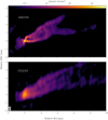 |
Fig. 1 M87: the posterior mean image by Bayesian self-calibration (top) and the self-calibrated CLEAN image (bottom) reconstructed from the same a-priori calibrated visibility data of VLBA observations at 43 GHz. In the figure, intensities higher than 3σrms (root mean square) of corresponding reconstruction were shown. The image obtained by resolve has Imax = 35 Jy mas−2 with the noise level of σrms = 2 mJy mas−2 which is calculated from the top left empty region in the posterior mean image. The CLEAN image restoring beam shown in the lower-left corner is 0.5×0.2 mas, Position angle (P.A.) = −11°. The CLEAN image has Imax = 6 Jy mas−2 with the noise level of σrms = 0.6 mJy mas−2. |
4.2 Reconstruction by CLEAN
We used DIFMAP (Shepherd 1997) software to reconstruct a Stokes I image using hybrid mapping in combination with superuniform, uniform and natural weighting with a pixel size of 0.03 milliarcsecond (mas) in Figure 1. Gain solutions from CLEAN self-calibration are shown in Figure C.2 and Figure C.3. The resulting image corresponds to the result obtained by Walker et al. (2018). To facilitate a direct comparison with the results obtained by the resolve software, we convert the standard CLEAN image intensity unit, originally in Jy/beam, to Jy mas−2. This conversion involved dividing the CLEAN output in Jy/beam by the beam area, which is calculated as  BMAJ ⋅ BMIN, where BMAJ and BMIN represent the major and minor axes of the beam, respectively. The noise level σrms = 67 µJy/beam was calculated 1 arcsecond from the phase center to minimize the influence of the bright VLBI core. Since CLEAN uses a conventional beam size, which does not always coincide with the effective resolution of the image, we display the CLEAN image convolved with 0.18 mas circular beam to show the resolved high flux density region. This “over-resolved” image is presented at the bottom of Figure F.2. The image helps to compare CLEAN result of high flux density region with the resolve result.
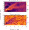 |
Fig. 2 M87: sky posterior pixel-wise standard deviation (top) and relative uncertainty, which is the sky posterior standard deviation normalized by the posterior mean (bottom) by resolve reconstruction from the top panel of Figure 1. |
4.3 Reconstruction by resolve
In Figure 1, the resolve posterior mean sky image is displayed. The resolve image is reconstructed with a spatial domain of 2048 × 1024 pixels and a field of view of 30 mas × 15 mas. The visibilities were time-averaged with a time interval of 10 seconds and frequency-averaged over 8 intermediate frequencies. For the resolve reconstruction, the number of data points is ≈1.5 × 10⁵ (RR and LL components) and we used 20 samples for the posterior estimation. As a result, the reduced χ2 value of the final result is 1.2, which ensures the consistency between the reconstruction results and the data. The wall-clock time for resolve run is 2h 40min on a single node of MPCDF Raven cluster with 20 MPI (Message Passing Interface) tasks.
In addition to the posterior mean image, the uncertainty of the image can be estimated from the sky posterior samples in resolve. In Figure 2, the shown relative uncertainty is the pixel-wise posterior standard deviation normalized by the sky posterior mean. We note that low relative uncertainty values are estimated in the core and limb-brightened jet regions.
During a conventional self-calibration for mm-VLBI data, low S/N data points and outliers are often flagged. However, it is often challenging to identify bad data points from data points inconsistent with the model image in self-calibration, and we therefore rely on expert’s experience. Data flagging without objective criteria hinders the reproducibility of results and biased prior knowledge might be imposed in image reconstruction owing to the manual data flagging. For the resolve self-calibration and imaging, data were only flagged by the rPI- CARD pipeline during pre-calibration and not flagged manually during Bayesian self-calibration and imaging in order to minimize human interaction. In Bayesian imaging, high uncertainty in low S/N data points is taken into account naturally during image reconstruction. Therefore, high-fidelity images can be reconstructed without manual data flagging in Bayesian framework, if adequate information of the noise level is available. Three percent of the visibility amplitude was added in the visibility noise as a systematic error budget, e.g., related to the uncalibrated polarimetric leakage (Event Horizon Telescope Collaboration 2019a).
The hyperparameter setup for log-sky ψ, log amplitude gain λ, and phase gain ϕ priors is described in Appendix C. Four temporal correlation kernels (amplitude gain and the phase gain for RCP and LCP mode respectively) are inferred under the assumption that antennas from homogeneous array have similar amplitude and phase gain correlation structures per polarization mode. We chose a resolution of 7054 pixels for the temporal domain of λ and ϕ and the time interval per each pixel is 10 seconds. We note that the time interval in gains is not directly related to the solution interval in CLEAN self-calibration method since the correlation structure is learned from the data automatically instead of using a fixed solution interval in resolve. We infer gain terms with two times of the observation time interval and crop only the first half since the Fast Fourier Transforms (FFT), which assumes periodicity, is utilized. The number of pixels for gain corrections is 7054 × 10 × 2 × 2 ≈ 2.8 × 10⁵ (2× observation interval × number of VLBI antennas × (phase, amplitude) × (RCP, LCP)). As a result, the degrees of freedom (DOF) for the inference are 2048 × 1024 + 7054 × 40 + power spectrum DOF ≈ 2.9 × 10⁶.
The posterior mean and standard deviation of amplitude and phase gains per each antenna and polarization mode are shown in Figures 3 and 4. The uncertainty of the amplitude and phase gain solutions is estimated by the posterior samples. Therefore, we can quantify the reliability of the amplitude and phase gain solutions by Bayesian self-calibration method. In order to validate the result, self-calibration solutions from CLEAN algorithm and an RML method by ehtim software (Chael et al. 2018) are shown in Appendices D and E. We note that resolve, CLEAN, and ehtim self-calibration solutions are comparable qualitatively, although different imaging methods and minimization schemes are employed. In Figures C.2 and C.3, there is no gain solution when we do not have data (BR: 7–8 h, HN: >8 h, MK: <2 h, NL: >9 h, and SC: >7 h). Gain solutions in those time intervals cannot be constrained by the data, standard deviations of the gain amplitude in Figure 3 are therefore increased.
Figures 5 and 6 show LCP and RCP gain solutions for Los Alamos (LA) and Saint Croix (SC) antenna, respectively. The amplitude and phase gain solutions are assumed to be smooth and to not very much. The amplitude gains vary up to 20% and the phase gains deviate up to 30 degrees. Considering temporal correlation in amplitude gain and phase gain solutions for this data is reasonable because the amplitude and phase coherence time of the VLBI array at 43 GHz is higher than 10 seconds.
Figure 1 shows two image reconstructions by the resolve and CLEAN. In the resolve image, better resolution is achived in the core and limb-brightened regions and the counter jet is more clear than CLEAN image. In Figure F.2, even the over-resolve CLEAN image cannot achieve the high resolution comparable with the resolve image. The extended jet emission looks more consistent in resolve image since the correlation structure between pixels are inferred by the Gaussian process prior with correlation kernel in resolve. Furthermore, the resolve image does not have negative flux because the positivity of the flux is enforced in the log-normal sky prior.
For the residual gain inference by resolve, the correlation structure between the gain solutions is inferred by the data. In other words, we do not need to choose solution interval of the gains manually but rather amplitude and phase gain solutions can be estimated by the Gaussian process prior model and more sophisticated inference scheme than the conventional CLEAN self-calibration. The consistency between data and the image with gain solutions is ensured since we fit the model to the data directly.
In order to obtain high-fidelity image, it is crucial to distinguish the uncertainty of gains and image from the VLBI data. From the perspective of statistical integrity, self-calibration and imaging should be performed simultaneously. Conventional iterative self-calibration estimates gain as a point and often flag outliers manually. This can impose a strong effective prior and thereby hinder proper accounting of the uncertainty information in the data. Furthermore, a variety of different images result from different ways CLEAN boxes are placed or different solution interval are chosen for amplitude and phase gains. Bayesian self-calibration and imaging can reduce such biases and provides reasonable uncertainty estimation of the gain solutions and image. This example with VLBA data set demonstrates that resolve is not only able to reconstruct images from real VLBI data but perform robust joint self-calibration and image reconstruction from sparse VLBI data set without iterative manual procedures.
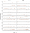 |
Fig. 3 M87: reconstructed posterior amplitude gains. The gain as a function of time is illustrated as a thin line with a semi-transparent standard deviation. The left and right columns of the figure show gains from the right (RCP) and left (LCP) circular polarizations correspondingly. Each row represents an individual antenna, whose abbreviated name is indicated in the bottom left corner of each LCP plot. |
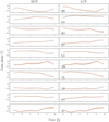 |
Fig. 4 M87: Reconstructed posterior phase gains. The gain as a function of time is illustrated as a thin line with a semi-transparent standard deviation. The left and right columns of the figure show gains from the right (RCP) and left (LCP) circular polarizations correspondingly. Each row represents an individual antenna, whose abbreviated name is indicated in the bottom left corner of each LCP plot. |
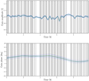 |
Fig. 5 M87: LCP amplitude (top) and phase (bottom) gain posterior mean and posterior samples for LA antenna by the Bayesian selfcalibration. The thick green solid line represents the posterior mean value, while the thin blue solid lines depict individual samples. Grey vertical shades indicate areas with available data points. |
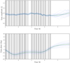 |
Fig. 6 M87: RCP amplitude (top) and phase (bottom) gain posterior mean and posterior samples for SC antenna by the Bayesian self-calibration. The thick green solid line represents the mean value, while the thin blue solid lines depict individual samples. Grey vertical shades indicate areas with available data points. |
5 Image reconstruction: synthetic data
5.1 Synthetic data
In order to validate the method, it is crucial to test the Bayesian self-calibration algorithm by applying it to synthetic visibility data with a known ground truth image. The synthetic data test is conducted in a semi-blind way. The metadata, including uv-coverage, frequency, and the error associated with each visibility point, was imported from the real observation data discussed in Section 4. For the ground truth image, we chose the 15GHz intensity image obtained by resolve using full-track VLBA May 2009 observations used in Nikonov et al. (2023). The ground truth image shows a great variety of scales from small and bright filaments to extended faint structures. To align the ground truth image with the real 43 GHz data, we scaled it down linearly to ensure that the jet lengths roughly correspond to each other. The resulting ground truth image is displayed in Figure 7. The uv-data was created from this image using ehtim software (Chael et al. 2019). To simulate the atmospheric, pointing and other antenna-based errors, we corrupted the data with periodic time-dependent complex antenna gains using CASA software. The periods of the gain functions for an individual antenna are defined between 1 and 12 hours to mimic inho-mogeneous statistics, which is commonly found in data from inhomogeneous arrays. The degree of gain variation was chosen based on the real observations, where one can observe the change of amplitude gain approximately 20% and for the phase around 10°.
5.2 Reconstruction by CLEAN and resolve
The CLEAN and resolve images with the synthetic data are depicted in Figure 7 and sky uncertainty maps are shown in Figure 8. The iterative self-calibration and image reconstruction setup by CLEAN are similar to the one discussed in Section 4.2. For Bayesian self-calibration and imaging by resolve, the hyper parameters of the log-sky prior ψ, log-amplitude gain prior λ, and phase gain prior ϕ for the synthetic data are the same as the reconstruction for the real data (in Tables C.1 and C.2). However, for all the antenna and their polarization modes, individual temporal correlation kernels for the amplitude and phase gains were employed for the synthetic data in order to infer gain corruptions with different correlation structures.
We choose a resolution of 2048 × 1024 pixels for the Stokes I image with a field of view 30 mas × 15 mas. The reduced χ2 of the resolve reconstruction with the synthetic data is 0.6.
Figure 7 shows a comparison of images of ground truth, CLEAN reconstruction, and resolve reconstruction. The CLEAN algorithm tends to reconstruct blobby extended structure since CLEAN reconstructs a collection of delta components and the delta components are convolved with the CLEAN beam to visualize the image. Furthermore, the core region is not optimally resolved even with over-resolved beam in Figure F.1. We note that multi-scale CLEAN might be able to recover the extended jet structure with better-resolved core, but iterative user-dependent self-calibration steps are still required in order to obtain high fidelity images. In the resolve image, the core and the extended jet structure in the ground truth image are recovered better than the CLEAN reconstruction.
The ground truth gain corruption and recovered resolve gain solution figures for the synthetic data are archived on zen-odo6. The reconstructed amplitude and phase gain solutions by the Bayesian self-calibration in the time coverage with data are reasonably consistent with the ground truth.
In conclusion, this example illustrates that a high fidelity image with robust amplitude and phase gain solutions with different correlation structure can be reconstructed from the corrupted synthetic data set by the Bayesian self-calibration and imaging method. Bayesian self-calibration may be utilized for inhomogeneous arrays, such as global mm-VLBI array (GMVA) and EVN (European VLBI network) to reconstruct reliable image and gain solutions with uncertainty estimation in the future.
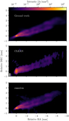 |
Fig. 7 Synthetic data: ground truth (top) and reconstructed images obtained using CLEAN (middle) and resolve (bottom) self-calibration. The restoring CLEAN beam illustrated in the bottom left corner of the plot is 0.5 × 0.2 mas, PA = −5°. All images in the figure were masked at 3σrms level of a corresponding image. The unified color bar on the top of the figure shows an intensity range of the ground truth (GT) image, where maximum intensity is |


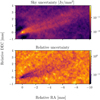 |
Fig. 8 Synthetic data: sky posterior pixel-wise standard deviation (top) and relative uncertainty, which is the sky posterior standard deviation normalized by the posterior mean (bottom) by resolve reconstruction from the bottom panel of Figure 7. |
6 Conclusion
We have presented the Bayesian self-calibration and imaging method by resolve and applied it to real and synthetic VLBI data. VLBA M87 data at 43 GHz were pre-calibrated by the rPI-CARD CASA-based pipeline and imaging with self-calibration was performed by Bayesian imaging software resolve. The data flagging was done by rPICARD pipeline without manual flagging and the image and gain solutions with uncertainty estimation were reconstructed jointly in the resolve framework.
Self-calibration solutions by resolve from real data are consistent with the conventional CLEAN and an RML method ehtim, despite the fact that different imaging approaches and gain inference schemes are utilized. In Bayesian self-calibration, we do not have to choose the solution interval of gain solutions but rather the time correlation structure of the gain solutions is inferred from the data. The synthetic data test shows that the Bayesian self-calibration method is able to infer different correlation structure of gain solutions per antenna and polarization mode, which is common in inhomogeneous VLBI arrays. Furthermore, in resolve, the uncertainty estimation of the gain solutions and image is provided on top of the posterior mean gains and image, which is important for the scientific analysis. On the other hand, in CLEAN self-calibration, residual gains are estimated and removed iteratively by using the CLEAN reconstructed model images as prior. Therefore, inconsistencies in the CLEAN model image resulting from user choices in the manual setting of CLEAN windows, weighting schemes, data flagging, and solution intervals for gain solutions may introduce bias. In RML-based ehtim self-calibration, the model image for self-calibration is consistent with the data since the model fits the data directly. However, solution interval is still chosen manually and only a point estimate of the antenna gain temporal evolution is provided, lacking any uncertainty information on the provided gain solution.
As a result, our example with the VLBA M87 data shows that we are able to reconstruct a robust image and antenna-based gain solutions with uncertainty estimation by taking into account the uncertainty information in the data. The VLBA M87 resolve image has better resolved core and counter jet, and consistent extended jet emission than the one provided by the conventional CLEAN reconstruction. This demonstrates the potential of the proposed method also for applications to other data sets. From our perspective, future work is needed on testing Bayesian self-calibration and imaging method on more challenging VLBI data, such as from sparse and inhomogeneous antenna array, and at high frequencies, and to incorporate polarization calibration in the resolve framework.
Data availability
The reduced image of M87 is available at the CDS via anonymous ftp to cdsarc.cds.unistra.fr (130.79.128.5) or via https://cdsarc.cds.unistra.fr/viz-bin/cat/J/A+A/690/A129
Supplementary material is available at https://zenodo.org/uploads/10190800
Acknowledgements
We thank the anonymous referee who suggested the validation with an RML-based method and constructive comments, Jack Livingston for feedback on drafts of the manuscript, Jakob Knollmüller for discussions on resolve software and feedback, Thomas Krichbaum and Martin Shepherd for discussions on CLEAN algorithm and DIFMAP software. J.K. and A.N. received financial support for this research from the International Max Planck Research School (IMPRS) for Astronomy and Astrophysics at the Universities of Bonn and Cologne. This work was supported by the M2FINDERS project funded by the European Research Council (ERC) under the European Union’s Horizon 2020 Research and Innovation Programme (Grant Agreement No. 101018682). J.R. acknowledges financial support from the German Federal Ministry of Education and Research (BMBF) under grant 05A23WO1 (Verbundprojekt D-MeerKAT III). P.A. acknowledges financial support from the German Federal Ministry of Education and Research (BMBF) under grant 05A20W01 (Verbundprojekt D-MeerKAT). The National Radio Astronomy Observatory is a facility of the National Science Foundation operated under cooperative agreement by Associated Universities, Inc.
Appendix A Weighting scheme in resolve
The statistics of the posterior sky distribution determined by Bayesian inference has some analogy to robust weighting in the CLEAN algorithm. The posterior distribution will include Fourier scales with high signal-to-noise, while Fourier scales with low signal-to-noise will be damped with the signal-to-noise ratio. This has some analogy to the CLEAN algorithm with robust weighting where Fourier scales with high signal-to-noise are uniformly weighted and scales with low signal-to-noise are weighted naturally. Nevertheless, in contrast to the CLEAN algorithm, this behavior of the resulting sky reconstruction is intrinsic to Bayesian inference or other methods following some form of regularized maximum likelihood approach.
In the appendix A.4 of Junklewitz et al. (2016), this analogy between robust weighting in CLEAN and the posterior obtained from Bayesian inference was made more explicit. More specifically, Junklewitz et al. (2016) derived the Bayesian Wiener Filter operation for estimating sky brightness, finding that it takes the same mathematical form of robust weighting when expressed in Fourier space. Thereby the robust parameter, which in the case of CLEAN needs to be chosen by the user is determined by the prior distribution for the sky brightness.
Appendix B Bayesian perspective on regularized maximum likelihood (RML) method
In this subsection, we aim to investigate the RML method from a Bayesian perspective. In the RML method, an objective function J(d, s) is to be minimized w.r.t. to the unknown signal s. Therefore, the RML estimator is
 (B.1)
(B.1)
The objective function consists of a data fidelity term χ2(d, s) and a regularizing term r(s,β) that should prevent irregular solutions (Chael et al. 2018):
 (B.2)
(B.2)
where β denotes the set of parameters the regularizer might depend on, including a potential parameter determining the relative weight of the regularization w.r.t. the data fidelity term.
The data fidelity term χ2(d, s) is equivalent to the likelihood Hamiltonian ℋ(d|s) in Bayesian inference up to irrelevant additive and multiplicative constants (see Eq. 12). In other words, the data fidelity term is the negavie log likelihood χ2(d, s) = – ln Ƥ(d|s) + const.. It is natural to regard the regularizing term r(s,β) as the negative log prior r(s,β) = − ln Ƥ(s|β) + const.. In this case, the RML estimator would be identical to the Bayesian maximum a posteriori (MAP) estimator for the corresponding signal prior Ƥ(s|β), with fixed hyperparameters β.
Therefore, RML method can be regarded as Bayesian methods in which the regularizing term r(s,β) specifies the prior assumption on the signal and that exploits the MAP approximation. From this perspective, the regularization terms can be translated into prior assumptions, via
 (B.3)
(B.3)
Here, the denominator in the last expression ensures proper normalization and would be essential to a Bayesian determination of the parameters β of the regularizer, which, however, is usually done in RML practice by trial and error and visual inspection of the results. We note that Müller et al. (2023) employed the genetic algorithm in order to automate the parameter βselection.
In RML methods, several regularizers are often combined in order to encode different prior knowledge about the source. Let us therefore revisit some of the commonly used regularizers in RML methods, such as the entropy, total variation (TV), and total squared variation (TSV) regularization and interpretation from the Bayesian perspective:
Entropy regularization of a discretized intensity field s(x, y) = I(x, y), with x,y ∈ ℤ, is given by
 (B.4)
(B.4)
with β = (T, M) consisting of a “temperature” T that determines the strength of the regularization and a reference image M, with respect to which this relative entropy like expression is evaluated. Converting this to a prior according to Eq. B.3 yields
 (B.5)
(B.5)
This means that all pixels are assumed to be uncorrelated, since the prior is a direct product of individual pixel priors
 (B.6)
(B.6)
These assign nearly constant probabilities for any flux value for which Ix,y << 1/T and a sharper than exponential cut off of the prior probabilities for intensities beyond Ix,y = 1/T. High flux values are therefore strongly suppressed by the entropy regularizer as was already pointed out by (Junklewitz et al. 2016).
Here, we would like to point out in addition to this that the reference image has a very mild effect on the results, as this super exponential cut off is fully determined by T. Approximately, the entropy regularization therefore corresponds to assuming the intensity field to be white noise with values roughly uniformly distributed between 0 and 1/T. For these reasons, the entropy RML is not expected to provide improved images for most radio astronomical observations of diffuse sources. The reputation of the entropy RML method to produce smooth images results probably from the usage of a large T parameter, which strongly discourages extreme brightnesses and therefore encourages the neighboring pixel of a strong flux location to explain the flux of that. A good feature of the entropy RML method is, however, that negative intensities are excluded by it a priori.
The total squared variation regularization
![${r_{{\rm{TSv}}}}(I,\beta ) = \alpha \sum\limits_{x,y} {\left[ {{{\left( {{I_{x + 1,y}} - {I_{x,y}}} \right)}^2} + {{\left( {{I_{x,y + 1}} - {I_{x,y}}} \right)}^2}} \right]} ,$](/articles/aa/full_html/2024/10/aa49663-24/aa49663-24-eq56.png) (B.7)
(B.7)
can be regarded in the continuum limit as requesting intensity gradients to be minimal
![${r_{{\rm{TSV}}}}(I,\beta ) \equiv {\alpha ^\prime }\int d x\int d y\left[ {{{\left( {{{\partial I(x,y)} \over {\partial x}}} \right)}^2} + {{\left( {{{\partial I(x,y)} \over {\partial y}}} \right)}^2}} \right]$](/articles/aa/full_html/2024/10/aa49663-24/aa49663-24-eq57.png) (B.8)
(B.8)
 (B.9)
(B.9)
where β = α in the discrete case and β = α′ in the corresponding continuum case determine the strength of the regularization.
The total squared variation regularization corresponds certainly to a more appropriate prior for diffuse emission, as it couples nearby locations and enforces some smoothness of the reconstruction.
This regularization actually becomes diagonal in Fourier space, with
 (B.10)
This turns out to be exactly (up to negligible additive terms) the log prior of a statistical homogeneous and isotropic Gaussian random field
 (B.11)
with an intensity power spectrum
 (B.12)
In one dimension, a Gaussian process with such a power spectrum would be equivalent to a Wiener process, which is known to produce continuous, but rough structures.
Changing to the total variation regularizer, in the continuum representation written as
 (B.13)
enhances the tendency to allow rough structures, but it favors roughness to be more localized. This is because the L1 norm underlying the TV regularizer is more tolerant to few large intensity gradients and the L2 norm underlying the TSV regularizer instead prefers many, smaller gradients. We note that the TSV regularizer does not have a simple Fourier space representation. Both, TV and TSV, regularizers are utilized to consider the correlation between neighboring pixels. However, they do not enforce the positivity of the sky intensity and tend to generate rough structures.
Appendix C Hyperparameter setup for sky and gain priors
Hyper parameters for the log-sky prior ψ.
The hyperparameter setup for the log-sky prior ψ is listed in Table C.1. The offset mean represents the mean value of the log-sky ψ; thus the mean of prior sky model exp(ψ) is exp(35) ≈ 1015 Jy/sr (≈ 10−2 Jy/mas2). The value is allowed to vary two e-folds up and down in one standard deviation (std) of the prior. The zero mode variance mean describes the standard deviation of the offset and its standard deviation is therefore the standard deviation of the offset standard deviation.
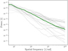 |
Fig. C.1 M87: posterior and prior power spectra of logarithmic sky brightness distribution ψ. The green line denotes posterior mean power spectrum; grey lines denote prior power spectrum samples. |
Hyper parameters for the log-amplitude gain prior λ and the phase gain prior ϕ.
The next four hyperparameters are model parameters for the spatial correlation power spectrum PΨ(ξΨ) in Eq. 24. The posterior and prior power spectra of the log-sky ψ are in Figure C.1. The average slope mean and std denote the mean and standard deviation of the slope for amplitude spectrum, which is the square root of the power spectrum. In Figure C.1, the prior power spectrum samples (grey lines) follow a power law with slope mean −6 and standard deviation 2. A steep prior power spectrum is chosen to suppress small scale structure in the early self-calibration stages. This prevents imprinting imaging artifacts from the noise to the final image. A relatively high standard deviation of the power spectrum is chosen to ensure flexibility of the prior model. Fluctuations and flexibility are non-trivial hyperparameters controlling the Wiener process and integrated Wiener process in the model, which determine fluctuation and flexibility of the power spectrum in a nonparametric fashion. Nonzero asperity can generate periodic patterns in the image. Thus, we used relatively small asperity parameters for our log-sky model ψ. We note that the power spectrum model is flexible enough to capture different correlation structures. As a result, the flexibility of the prior model can reduce biases from strong prior assumptions.
For the self-calibration of the real data (see Section 4.3), four temporal correlation kernels (amplitude gain and the phase gain for RCP and LCP mode respectively) are inferred under the assumption that antennas from homogeneous array have similar amplitude and phase gain correlation structures per polarization mode. For the self-calibration of the synthetic data (see Section 5.2), 40 individual temporal correlation kernels for the amplitude and phase gains are inferred, one per antenna and polarization mode, as the ground truth gain corruptions were generated with individual correlation structures. The mean of the amplitude gain prior model is obtained by exponentiating the offset mean of λ, which is exp(0) = 1 and the mean of the phase gain prior model is the offset mean of ϕ, which is 0 radians. Model parameters for the zero mode variance, fluctuations, and flexibility are chosen to be small to suppress extremely high gain corrections. Asperity mean and std hyper parameters are set to None since the gain solutions are not periodic. The average slope mean is −3 for log-amplitude and phase gain, therefore the slope mean for the power spectrum is −6 with the standard deviataion 2. The broad range of the average slope parameter allows the prior model to describe different temporal correlation structures. As a result, the gain prior model is flexible enough to learn the temporal correlation structure from the data automatically. More details about prior model parameters are explained in Arras et al. (2021).
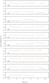 |
Fig. C.2 Real data: Amplitude gain solutions by the CLEAN self-calibration method. |
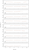 |
Fig. C.3 Real data: Phase gain solutions by the CLEAN self-calibration method. |
Appendix D CLEAN self-calibration solutions: real data
Figure C.2 and Figure C.3 show the CLEAN self-calibration solutions for the real VLBI M87 data at 43GHz by DIFMAP software. One amplitude and one phase gain solution per each antenna are obtained because CLEAN image in Figure 1 is produced by the Stokes I data averaging the RR and LL components. Since the Stokes V emission is negligible in the data, resolve gain solutions for RCP and LCP are very similar in Figure 3 and Figure 4. Therefore, a high-fidelity total intensity image can be reconstructed by estimating one gain solution per each antenna in CLEAN self-calibration.
We can compare self-calibration solutions from CLEAN and resolve. The gain solutions from CLEAN and resolve with scans are consistent qualitatively. As an example, the abrupt variation of the resolve gain amplitude for LA antenna (6h −6.5h) in Figure 5 is due to the discrepancy of amplitude between scans. Figure C.2 shows a similar behavior in the CLEAN gain amplitude for LA antenna (6h - 6.5h). We note that the data were flagged manually during CLEAN self-calibration. Outliers are often flagged during iterative CLEAN self-calibration and the data flagging relies on user’s experience. On the other hand, in resolve self-calibration, the whole data after pre-calibration are used for imaging without manual flagging.
Appendix E ehtim image and self-calibration solutions: real data
ehtim (Chael et al. 2018) is a widely used RML imaging software for VLBI data, e.g. by the Event Horizon Telescope at 230 GHz (e.g. Event Horizon Telescope Collaboration 2019b; The Event Horizon Telescope Collaboration 2023; Event Horizon Telescope Collaboration 2024), for observations with the global Millimeter VLBI Array (GMVA) at 86 GHz (e.g. Zhao et al. 2022), observations with European VLBI network (EVN), the Very Long Baseline Array (VLBA), and the space VLBI mission RadioAstron at smaller frequencies (e.g. recently Kosogorov et al. 2024; Paraschos et al. 2024; Fuentes et al. 2023), and even for related inverse problems outside of radio astronomy (Müller et al. 2024). To validate the resolve self-calibration and imaging method, we compare it to RML self-calibration and imaging performed by ehtim. The comparison of resolve and ehtim image is shown in Figure E.1. ehtim minimizes a weighted sum of data terms (chosen to be χ1 -terms based on visibilities), and regularization terms (entropy, TV, TSV, l1-norm, total flux constraint). To navigate this large number of parameters, usually either a parameter survey (e.g. Event Horizon Telescope Collaboration 2019b; Fuentes et al. 2023) or metaheuristics (Müller et al. 2023; Mus et al. 2024) are applied to ehtim. Performing a full exploration of the parameter space would exceed the scope of this comparison. Hence, for this work, we rather chose the regularization weights by manual exploration to the best of our efforts.
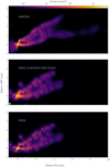 |
Fig. E.1 Real data: resolve image (top), ehtim image convolved with the beam (0.167 mas × 0.167 mas, middle), and ehtim image (bottom). The beam-convolved ehtim image (middle) has Imax = 14 Jy mas−2 and ehtim image (bottom) has Imax = 73 Jy mas−2. |
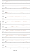 |
Fig. E.2 Real data: Amplitude gain solutions by the ehtim self-calibration method. |
In ehtim, the self-calibration procedure is similar to CLEAN self-calibration. First, a model image is reconstructed by the given data. Second, residual gains are estimated by minimizing a cost function (Eq. 18) based on the Fourier components of the model image. Then new data are generated by removing the estimated residual gain corruption. These procedures are continued iteratively until the desired image quality is achieved. In contrast to the CLEAN self-calibration, the model images computed by ehtim can be consistent with data since the model fits the data directly in the visibility domain.
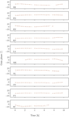 |
Fig. E.3 Real data: Phase gain solutions by the ehtim self-calibration method. |
The ehtim image in Figure E.1 achieves better resolution compared to CLEAN image in Figure 1. The core regions show even sharper edge-brightening and counter jet than resolve image. However, the image contains sharper artifacts in the core region and the extended jet emission looks discontinuous. Therefore, we convolved ehtim image with the beam (0.167mas × 0.167mas) to show an image at a conservative resolution. The core, counter jet, and extended jet emission in resolve and beam-convolved ehtim images look consistent. We note that the smoothness of the image is enforced by the TV and TSV regularizes in ehtim reconstruction. However, since TV and TSV regularizers tend to produce rough structures (see Appendix B), these regularizers may not be optimal for recovering extended jet emission as ehtim was developed for the high-resolution reconstruction of compact emission. It has been demonstrated in the past that the use of extended basis functions, rather than regularizers acting in the pixel basis, may offer an advantage for these cases in RML methods (see the SARA family Carrillo et al. 2012; Terris et al. 2023; Wilber et al. 2023).
Figure E.2 and Figure E.3 show the amplitude and phase gain solutions by ehtim self-calibration. Self-calibration by ehtim is performed alternating with the deconvolution. For the self-calibration of real M87 data, no temporal correlation between gain solutions is considered and small gain tolerance of (0.01, 0.05) is used to correct the gain incrementally. This means that both, gains smaller than 0.01 and larger than 0.05, are disfavored by the prior. We detect gain phase and amplitude trends that are consistent with the results obtained with resolve and CLEAN.
Appendix F Comparison of resolve and over-resolved CLEAN image
Figure F.1 and Figure F.2 show the comparison between CLEAN image with over-resolved beam and resolve image with saturated color bar for synthetic and real data respectively. In Figure F.1, the CLEAN algorithm is not able to recover small scale structures in the core of the ground truth image even with over-resolved beam. Furthermore, the extended jet in CLEAN image is discontinuous due to the small size of the CLEAN beam. In resolve image, the extended jet and bright core are relatively well recovered. We note that a prominent central spine in extended jet is reconstructed in CLEAN image. It is not pronounced in the ground truth image, can therefore be CLEAN artifacts (Pashchenko et al. 2023). In Figure F.2, the structure of core and limb-brightened region is consistent in resolve and CLEAN reconstruction with over-resolved beam. The central spine in extended jet is pronounced in the CLEAN image again, same as the CLEAN reconstruction from the synthetic data.
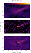 |
Fig. F.1 Synthetic data: ground truth (top) and reconstructed images obtained using CLEAN (middle) and resolve (bottom) self-calibration. The circular 0.15 mas CLEAN beam is illustrated in the bottom left corner of the plot. The CLEAN image was masked at the lowest positive value. The unified color bar on the top of the figure shows an intensity range of the ground truth image, where maximum intensity is |


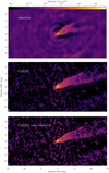 |
Fig. F.2 M87: the posterior mean image by Bayesian self-calibration (top), the self-calibrated CLEAN image (middle) and the over-resolved CLEAN image (bottom) reconstructed from the same a-priori calibrated visibility data of VLBA observations at 43 GHz. The unified color bar shows an intensity range from the minimum intensity up to the maximum intensity of the resolve image. The image obtained by the Bayesian approach has a maximum intensity Imax = 35 Jy mas−2 with a minimum value of Imin = 8 µJy mas−2. The CLEAN image (middle) restoring beam shown in the lower-left corner of the plot is 0.5 × 0.2 mas, P.A. = −11°. The maximum intensity of the CLEAN reconstruction is Imax = 6 Jy mas−2. The over-resolved CLEAN image (bottom) circular restoring beam shown in the lower-left corner of the plot is 0.18 mas. The maximum intensity of the over-resolved CLEAN image is Ipeak = 13 Jy mas−2. |
References
- Akiyama, K., Ikeda, S., Pleau, M., et al. 2017, AJ, 153, 159 [NASA ADS] [CrossRef] [Google Scholar]
- Arras, P., Baltac, M., Ensslin, T. A., et al. 2019a, NIFTy5: Numerical Information Field Theory v5, Astrophysics Source Code Library [record ascl:1903.008] [Google Scholar]
- Arras, P., Frank, P., Leike, R., Westermann, R., & Enßlin, T. A. 2019b, A&A, 627, A134 [NASA ADS] [CrossRef] [EDP Sciences] [Google Scholar]
- Arras, P., Bester, H. L., Perley, R. A., et al. 2021, A&A, 646, A84 [NASA ADS] [CrossRef] [EDP Sciences] [Google Scholar]
- Arras, P., Frank, P., Haim, P., et al. 2022, Nat. Astron., 6, 259 [NASA ADS] [CrossRef] [Google Scholar]
- Blei, D. M., Kucukelbir, A., & McAuliffe, J. D. 2016, arXiv e-prints [arXiv: 1601.00670] [Google Scholar]
- Broderick, A. E., Gold, R., Karami, M., et al. 2020, ApJ, 897, 139 [Google Scholar]
- Brogan, C. L., Hunter, T. R., & Fomalont, E. B. 2018, arXiv e-prints [arXiv: 1805.05266] [Google Scholar]
- Carrillo, R. E., McEwen, J. D., & Wiaux, Y. 2012, MNRAS, 426, 1223 [Google Scholar]
- Chael, A. A., Johnson, M. D., Bouman, K. L., et al. 2018, ApJ, 857, 23 [Google Scholar]
- Chael, A. A., Bouman, K. L., Johnson, M. D., et al. 2019, ehtim: Imaging, analysis, and simulation software for radio interferometry, Astrophysics Source Code Library [record ascl:1904.004] [Google Scholar]
- Clark, B. G. 1980, A&A, 89, 377 [NASA ADS] [Google Scholar]
- Cornwell, T. J. 2008, IEEE J. Sel. Top. Signal Process., 2, 793 [Google Scholar]
- Cornwell, T. J., & Evans, K. F. 1985, A&A, 143, 77 [NASA ADS] [Google Scholar]
- Cornwell, T. J., & Wilkinson, P. N. 1981, MNRAS, 196, 1067 [NASA ADS] [Google Scholar]
- Dabbech, A., Repetti, A., Perley, R. A., Smirnov, O. M., & Wiaux, Y. 2021, MNRAS, 506, 4855 [NASA ADS] [CrossRef] [Google Scholar]
- Enßlin, T. A. 2019, Ann. Phys., 531, 1800127 [Google Scholar]
- Enßlin, T. A., & Frommert, M. 2011, Phys. Rev. D, 83, 105014 [Google Scholar]
- Event Horizon Telescope Collaboration (Akiyama, K., et al.) 2019a, ApJ, 875, L3 [Google Scholar]
- Event Horizon Telescope Collaboration (Akiyama, K., et al.) 2019b, ApJ, 875, L4 [Google Scholar]
- Event Horizon Telescope Collaboration (Akiyama, K., et al.) 2024, A&A, 681, A79 [NASA ADS] [CrossRef] [EDP Sciences] [Google Scholar]
- Frank, P., Leike, R., & Enßlin, T. A. 2021a, Ann. Phys., 533, 2000486 [NASA ADS] [CrossRef] [Google Scholar]
- Frank, P., Leike, R., & Enßlin, T. A. 2021b, Entropy, 23, 853 [NASA ADS] [CrossRef] [Google Scholar]
- Fuentes, A., Gómez, J. L., Martí, J. M., et al. 2023, Nat. Astron., 7, 1359 [NASA ADS] [CrossRef] [Google Scholar]
- Hamaker, J. P., Bregman, J. D., & Sault, R. J. 1996, A&AS, 117, 137 [NASA ADS] [CrossRef] [EDP Sciences] [Google Scholar]
- Högbom, J. A. 1974, A&AS, 15, 417 [Google Scholar]
- Janssen, M., Goddi, C., van Bemmel, I. M., et al. 2019, A&A, 626, A75 [NASA ADS] [CrossRef] [EDP Sciences] [Google Scholar]
- Janssen, M., Radcliffe, J. F., & Wagner, J. 2022, Universe, 8, 527 [NASA ADS] [CrossRef] [Google Scholar]
- Junklewitz, H., Bell, M. R., & Enßlin, T. 2015, A&A, 581, A59 [NASA ADS] [CrossRef] [EDP Sciences] [Google Scholar]
- Junklewitz, H., Bell, M. R., Selig, M., & Enßlin, T. A. 2016, A&A, 586, A76 [NASA ADS] [CrossRef] [EDP Sciences] [Google Scholar]
- Khinchin, A. 1934, Math. Ann., 109, 604 [CrossRef] [Google Scholar]
- Knollmüller, J., & Enßlin, T. A. 2018, arXiv e-prints [arXiv: 1812.04403] [Google Scholar]
- Knollmüller, J., & Enßlin, T. A. 2019, arXiv e-prints [arXiv:1901.11033] [Google Scholar]
- Kosogorov, N. A., Kovalev, Y. Y., Perucho, M., & Kovalev, Y. A. 2024, MNRAS, 528, 1697 [NASA ADS] [CrossRef] [Google Scholar]
- Martí-Vidal, I., & Marcaide, J. M. 2008, A&A, 480, 289 [CrossRef] [EDP Sciences] [Google Scholar]
- Müller, H., & Lobanov, A. P. 2022, A&A, 666, A137 [NASA ADS] [CrossRef] [EDP Sciences] [Google Scholar]
- Müller, H., Mus, A., & Lobanov, A. 2023, A&A, 675, A60 [NASA ADS] [CrossRef] [EDP Sciences] [Google Scholar]
- Müller, H., Massa, P., Mus, A., Kim, J.-S., & Perracchione, E. 2024, A&A, 684, A47 [NASA ADS] [CrossRef] [EDP Sciences] [Google Scholar]
- Mus, A., Müller, H., & Lobanov, A. 2024, A&A, 688, A100 [NASA ADS] [CrossRef] [EDP Sciences] [Google Scholar]
- Narayan, R., & Nityananda, R. 1986, ARA&A, 24, 127 [Google Scholar]
- Nikonov, A. S., Kovalev, Y. Y., Kravchenko, E. V., Pashchenko, I. N., & Lobanov, A. P. 2023, MNRAS, 526, 5949 [NASA ADS] [CrossRef] [Google Scholar]
- Paraschos, G. F., Debbrecht, L. C., Kramer, J. A., et al. 2024, A&A, 686, L5 [NASA ADS] [CrossRef] [EDP Sciences] [Google Scholar]
- Pashchenko, I. N., Kravchenko, E. V., Nokhrina, E. E., & Nikonov, A. S. 2023, MNRAS, 523, 1247 [NASA ADS] [CrossRef] [Google Scholar]
- Popkov, A. V., Kovalev, Y. Y., Petrov, L. Y., & Kovalev, Y. A. 2021, AJ, 161, 88 [CrossRef] [Google Scholar]
- Roth, J., Arras, P., Reinecke, M., et al. 2023, A&A, 678, A177 [NASA ADS] [CrossRef] [EDP Sciences] [Google Scholar]
- Shepherd, M. C. 1997, in Astronomical Society of the Pacific Conference Series, 125, Astronomical Data Analysis Software and Systems VI, eds. G. Hunt, & H. Payne, 77 [NASA ADS] [Google Scholar]
- Smirnov, O. M. 2011, A&A, 527, A106 [NASA ADS] [CrossRef] [EDP Sciences] [Google Scholar]
- Taylor, G. B., Carilli, C. L., & Perley, R. A. 1999, Astronomical Society of the Pacific Conference Series, 180, Synthesis Imaging in Radio Astronomy II [Google Scholar]
- Terris, M., Dabbech, A., Tang, C., & Wiaux, Y. 2023, MNRAS, 518, 604 [Google Scholar]
- The Event Horizon Telescope Collaboration 2023, arXiv e-prints [arXiv:2311.09479] [Google Scholar]
- Thompson, A. R., Moran, J. M., & Swenson, George W., J. 2017, Interferometry and Synthesis in Radio Astronomy, 3rd edn (Springer Cham) [Google Scholar]
- Tiede, P. 2022, J. Open Source Softw., 7, 4457 [NASA ADS] [CrossRef] [Google Scholar]
- Walker, R. C., Hardee, P. E., Davies, F. B., Ly, C., & Junor, W. 2018, ApJ, 855, 128 [Google Scholar]
- Wiaux, Y., Jacques, L., Puy, G., Scaife, A. M. M., & Vandergheynst, P. 2009, MNRAS, 395, 1733 [NASA ADS] [CrossRef] [Google Scholar]
- Wiener, H. 1949, Extrapolation, Interpolation, and Smoothing of Stationary Time Series, with Engineering Applications (MIT Press) [CrossRef] [Google Scholar]
- Wilber, A. G., Dabbech, A., Jackson, A., & Wiaux, Y. 2023, MNRAS, 522, 5558 [NASA ADS] [CrossRef] [Google Scholar]
- Zhao, G.-Y., Gómez, J. L., Fuentes, A., et al. 2022, ApJ, 932, 72 [NASA ADS] [CrossRef] [Google Scholar]
https://hub.docker.com/r/mjanssen2308/casavlbi The container corresponding to v7.1.2 is tagged as ec77b9874a6de7d071c8a1d8b3816702d4c6fd9f.
All Tables
Hyper parameters for the log-amplitude gain prior λ and the phase gain prior ϕ.
All Figures
|
Fig. 1 M87: the posterior mean image by Bayesian self-calibration (top) and the self-calibrated CLEAN image (bottom) reconstructed from the same a-priori calibrated visibility data of VLBA observations at 43 GHz. In the figure, intensities higher than 3σrms (root mean square) of corresponding reconstruction were shown. The image obtained by resolve has Imax = 35 Jy mas−2 with the noise level of σrms = 2 mJy mas−2 which is calculated from the top left empty region in the posterior mean image. The CLEAN image restoring beam shown in the lower-left corner is 0.5×0.2 mas, Position angle (P.A.) = −11°. The CLEAN image has Imax = 6 Jy mas−2 with the noise level of σrms = 0.6 mJy mas−2. |
| In the text | |
|
Fig. 2 M87: sky posterior pixel-wise standard deviation (top) and relative uncertainty, which is the sky posterior standard deviation normalized by the posterior mean (bottom) by resolve reconstruction from the top panel of Figure 1. |
| In the text | |
|
Fig. 3 M87: reconstructed posterior amplitude gains. The gain as a function of time is illustrated as a thin line with a semi-transparent standard deviation. The left and right columns of the figure show gains from the right (RCP) and left (LCP) circular polarizations correspondingly. Each row represents an individual antenna, whose abbreviated name is indicated in the bottom left corner of each LCP plot. |
| In the text | |
|
Fig. 4 M87: Reconstructed posterior phase gains. The gain as a function of time is illustrated as a thin line with a semi-transparent standard deviation. The left and right columns of the figure show gains from the right (RCP) and left (LCP) circular polarizations correspondingly. Each row represents an individual antenna, whose abbreviated name is indicated in the bottom left corner of each LCP plot. |
| In the text | |
|
Fig. 5 M87: LCP amplitude (top) and phase (bottom) gain posterior mean and posterior samples for LA antenna by the Bayesian selfcalibration. The thick green solid line represents the posterior mean value, while the thin blue solid lines depict individual samples. Grey vertical shades indicate areas with available data points. |
| In the text | |
|
Fig. 6 M87: RCP amplitude (top) and phase (bottom) gain posterior mean and posterior samples for SC antenna by the Bayesian self-calibration. The thick green solid line represents the mean value, while the thin blue solid lines depict individual samples. Grey vertical shades indicate areas with available data points. |
| In the text | |
|
Fig. 7 Synthetic data: ground truth (top) and reconstructed images obtained using CLEAN (middle) and resolve (bottom) self-calibration. The restoring CLEAN beam illustrated in the bottom left corner of the plot is 0.5 × 0.2 mas, PA = −5°. All images in the figure were masked at 3σrms level of a corresponding image. The unified color bar on the top of the figure shows an intensity range of the ground truth (GT) image, where maximum intensity is |
| In the text | |
|
Fig. 8 Synthetic data: sky posterior pixel-wise standard deviation (top) and relative uncertainty, which is the sky posterior standard deviation normalized by the posterior mean (bottom) by resolve reconstruction from the bottom panel of Figure 7. |
| In the text | |
|
Fig. C.1 M87: posterior and prior power spectra of logarithmic sky brightness distribution ψ. The green line denotes posterior mean power spectrum; grey lines denote prior power spectrum samples. |
| In the text | |
|
Fig. C.2 Real data: Amplitude gain solutions by the CLEAN self-calibration method. |
| In the text | |
|
Fig. C.3 Real data: Phase gain solutions by the CLEAN self-calibration method. |
| In the text | |
|
Fig. E.1 Real data: resolve image (top), ehtim image convolved with the beam (0.167 mas × 0.167 mas, middle), and ehtim image (bottom). The beam-convolved ehtim image (middle) has Imax = 14 Jy mas−2 and ehtim image (bottom) has Imax = 73 Jy mas−2. |
| In the text | |
|
Fig. E.2 Real data: Amplitude gain solutions by the ehtim self-calibration method. |
| In the text | |
|
Fig. E.3 Real data: Phase gain solutions by the ehtim self-calibration method. |
| In the text | |
|
Fig. F.1 Synthetic data: ground truth (top) and reconstructed images obtained using CLEAN (middle) and resolve (bottom) self-calibration. The circular 0.15 mas CLEAN beam is illustrated in the bottom left corner of the plot. The CLEAN image was masked at the lowest positive value. The unified color bar on the top of the figure shows an intensity range of the ground truth image, where maximum intensity is |
| In the text | |
|
Fig. F.2 M87: the posterior mean image by Bayesian self-calibration (top), the self-calibrated CLEAN image (middle) and the over-resolved CLEAN image (bottom) reconstructed from the same a-priori calibrated visibility data of VLBA observations at 43 GHz. The unified color bar shows an intensity range from the minimum intensity up to the maximum intensity of the resolve image. The image obtained by the Bayesian approach has a maximum intensity Imax = 35 Jy mas−2 with a minimum value of Imin = 8 µJy mas−2. The CLEAN image (middle) restoring beam shown in the lower-left corner of the plot is 0.5 × 0.2 mas, P.A. = −11°. The maximum intensity of the CLEAN reconstruction is Imax = 6 Jy mas−2. The over-resolved CLEAN image (bottom) circular restoring beam shown in the lower-left corner of the plot is 0.18 mas. The maximum intensity of the over-resolved CLEAN image is Ipeak = 13 Jy mas−2. |
| In the text | |
Current usage metrics show cumulative count of Article Views (full-text article views including HTML views, PDF and ePub downloads, according to the available data) and Abstracts Views on Vision4Press platform.
Data correspond to usage on the plateform after 2015. The current usage metrics is available 48-96 hours after online publication and is updated daily on week days.
Initial download of the metrics may take a while.