| Issue |
A&A
Volume 690, October 2024
|
|
|---|---|---|
| Article Number | A384 | |
| Number of page(s) | 15 | |
| Section | Astrophysical processes | |
| DOI | https://doi.org/10.1051/0004-6361/202449481 | |
| Published online | 24 October 2024 | |
Strong lensing of tidal disruption events: Detection rates in imaging surveys
1
Max-Planck-Institut für Astrophysik, Karl-Schwarzschild Str. 1, 85741 Garching, Germany
2
Physics and Astronomy Department, Johns Hopkins University, Baltimore, MD 21218, USA
3
Technical University of Munich, TUM School of Natural Sciences, Department of Physics, James-Franck-Straße 1, 85748 Garching, Germany
4
Institute of Astronomy and Astrophysics, Academia Sinica, 11F of ASMAB, No.1, Section 4, Roosevelt Road, Taipei 10617, Taiwan
5
Center for Frontier Science, Chiba University, 1-33 Yayoi-cho, Inage-ku, Chiba 263-8522, Japan
6
Department of Physics, Graduate School of Science, Chiba University, 1-33 Yayoi-Cho, Inage-Ku, Chiba 263-8522, Japan
7
Department of Physics, University of Hong Kong, Pokfulam Road, Hong Kong
⋆ Corresponding author; This email address is being protected from spambots. You need JavaScript enabled to view it.
Received:
3
February
2024
Accepted:
1
June
2024
Abstract
Tidal disruption events (TDEs) are multi-messenger transients in which a star is tidally destroyed by a supermassive black hole at the center of galaxies. The Rubin Observatory Legacy Survey of Space and Time (LSST) is anticipated to detect hundreds to thousands of TDEs annually, such that the first gravitationally lensed TDE may be observed in the coming years. Using Monte-Carlo simulations, we quantify the rate of both unlensed and lensed TDEs as a function of limiting magnitudes in four different optical bands (u, g, r, and i) for a range of TDE temperatures that match observations. Dependent on the temperature and luminosity model, we find that g and r bands are the most promising bands with unlensed TDE detections that can be as high as ∼104 annually. By populating a cosmic volume with realistic distributions of TDEs and galaxies that can act as gravitational lenses, we estimate that a few lensed TDEs (depending on the TDE luminosity model) can be detected annually in g or r bands in the LSST survey, with TDE redshifts in the range of ∼0.5 to ∼2. The ratio of lensed to unlensed detections indicates that we may detect ∼1 lensed event for every 104 unlensed events, which is independent of the luminosity model. The number of lensed TDEs decreases as a function of the image separations and time delays, and most of the lensed TDE systems are expected to have image separations below ∼3″ and time delays within ∼30 days. At fainter limiting magnitudes, the i band becomes notably more successful. These results suggest that strongly lensed TDEs are likely to be observed within the coming years and such detections will enable us to study the demographics of black holes at higher redshifts through the lensing magnifications. Our simulated catalogs of lensed TDEs are publicly available.
Key words: gravitational lensing: strong / galaxies: general / galaxies: nuclei / quasars: supermassive black holes
© The Authors 2024
 Open Access article, published by EDP Sciences, under the terms of the Creative Commons Attribution License (https://creativecommons.org/licenses/by/4.0), which permits unrestricted use, distribution, and reproduction in any medium, provided the original work is properly cited.
This article is published in open access under the Subscribe to Open model.
Open Access funding provided by Max Planck Society.
1. Introduction
Tidal disruption events (TDEs) occur when a star passes sufficiently close to a supermassive black hole (SMBH) such that the tidal forces of the black hole (BH) overcome the star’s self gravity, and the star is subsequently disrupted (Hills 1988; Rees 1988), generating a flare that is detectable on the time scale of a few months to a few years (e.g., Gezari 2021). Since quiescent BHs can create TDEs, TDEs can serve as a promising tool for probing these dormant BHs. The population studies of TDEs in dwarf galaxies will provide a better understanding of the BH mass function. Currently, on the order of 100 TDE candidates have been detected with a typical redshift of z ≲ 0.2, but this number will exponentially grow to possibly more than thousands with detections by ongoing (e.g., Zwicky Transient Facility (ZTF; Bellm 2014) and eROSITA (Predehl et al. 2021)) and upcoming surveys (e.g., Rubin Observatory Legacy Survey of Space and Time (LSST; Ivezić et al. 2019) and Ultraviolet Transient Astronomy Satellite (ULTRASAT; Shvartzvald et al. 2024).
Although the detections of TDEs so far have been confined within the nearby universe, TDEs at cosmological distances could be detected in the future with observing instruments with deeper fields. For that case, it is possible these events can be gravitationally lensed by galaxies at lower redshifts, magnifying the brightness of the TDEs. Such lensing effects would enable the detections of TDEs at even higher redshifts, which would allow us to study the TDE rates and the BH mass function at the lower mass end and at earlier cosmic time. Additionally, through studying the microlensing of TDEs, we can obtain an independent constraint on the size of the TDE emitting region which can help to identify its emission mechanism (as demonstrated in studies of active galactic nuclei (AGNs) with their accretion disk sizes measured through microlensing, e.g., Kochanek 2004; Schmidt & Wambsganss 2010; Blackburne et al. 2014).
In fact, the strongly lensed detection rates have been estimated for quasars (a type of AGN) and supernovae for various surveys (e.g., LSST and Supernova Legacy Survey (SNLS)) (e.g., Oguri & Marshall 2010; Wojtak et al. 2019; Goldstein et al. 2019; Arendse et al. 2024). Specifically, Oguri & Marshall (2010) populated a region of their simulation with lens galaxies and either quasars or supernovae by randomly assigning redshifts to both objects and a magnitude to the source based on their luminosity and mass functions. They then computed the lensing effects for every source in the simulation and determined if the strongly lensed system will be detected by the particular survey. Through these simulations, Oguri & Marshall (2010) estimate ∼3000 lensed quasars and ∼100 lensed supernovae will be detectable with LSST. By considering different detection algorithms (such as through lensing magnifications instead of multiplicity of lensed images) and also observing cadence, other studies estimate even higher rates, up to ∼1000 (Wojtak et al. 2019; Goldstein et al. 2019; Arendse et al. 2024). TDEs, although rarer than supernovae and quasars, could potentially be strongly lensed and detected in LSST as well.
As the number of detected TDEs is expected to grow in the coming years, it is important to quantify how many lensed TDEs may be detected by full sky surveys. We focus on calculating the strongly lensed TDE detection rates in this paper. As a first step, using the code developed by Oguri & Marshall (2010), we estimate the strongly lensed TDE detection rates over a wide range of limiting magnitudes and blackbody temperatures assuming two luminosity models which bracket the range of observed TDE luminosities. We then choose the blackbody temperature that best corresponds with current ZTF observations. Then, using the chosen temperature model, we compute the strongly lensed TDE detection rates for both luminosity cases. We use the range of detection rates from the two luminosity models to provide a bound on the strongly lensed detection rate.
Recently, Chen et al. (2024) have independently estimated the rates of strongly lensed TDEs through simulations of TDE light curves and computations of lensing probabilities. Our results on the lensed TDE rates are overall consistent with the lower end of the range predicted by Chen et al. (2024), although the details of models and criteria used for detection are different, which we discuss further in Sect. 4.
This paper is organized as follows. We provide the descriptions for our methodology and present the estimated unlensed TDE rates in Sect. 2. Then, we explain our strategies for estimating lensed rates in Sect. 3. In this section, we give our estimates of the lensed TDE rates, and show the distributions of the lens properties from the resulting strongly lensed systems. We discuss some of the caveats of this work in Sect. 4, and we conclude in Sect. 5. Magnitudes in this paper are in the AB system.
2. Detection rates of unlensed TDEs
In this section, we compute the rates of TDEs based on theoretical models that are matched to observations. We begin in Sect. 2.1 with an overview of our computation of the rates, and we detail the ingredients for this computation in Sects. 2.2–2.4. Our results of the detection rates of TDEs are presented in Sect. 2.5.
2.1. Overview of method
We calculated the detection rates of unlensed TDEs for each X band (X = u, g, r, i) by performing the following integral,
 (1)
(1)
where ψTDE is the TDE luminosity function as a function of magnitude mX detected in the X band and dV/dz is the cosmological volume element (see Eq. (8) in Oguri & Marshall (2010)) assuming (Ωm, ΩΛ) = (0.3, 0.7) and H0 = 72 km s−1 Mpc−1. The upper bound mmin is determined by the brightest event, and mmax is set by the smaller of either the faintest event or the filter magnitude limit. The zmax bound is determined by the TDE with the highest luminosity contained within the filter magnitude limit. To compute ψTDE(mX)dmX, we first constructed ψTDE(MBH) as a function of BH mass, MBH, from the BH mass function, ϕBH, and the TDE rate per galaxy, Γ (see Sect. 2.2). Then, we converted ψTDE(MBH) into ψTDE(L) as a function of luminosity, L, assuming two different TDE luminosities (see Sect. 2.3). Finally, we converted ψTDE(L) into ψTDE(mX) for different bands assuming black body emissions (see Sect. 2.4).
We computed these unlensed detection rates for a range of constant temperatures and compared with current ZTF detections to determine the model that best corresponds with observations. We estimated these rates, and later the lensed detection rates, for the X = u, g, r, i LSST bands. We did not consider the z, y bands given that they are further into the infrared, so the detection rates in these two bands are expected to be low, since TDEs are optically bright, unless the TDEs are at a high enough redshift. Additionally, we showed how the rates evolve with a variable magnitude cutoff assuming a particular survey area of 20 000 deg2. In this way, the annual detection rates in any imaging survey can be estimated given its magnitude limit.
2.2. Luminosity function - ψTDE(MBH)dMBH
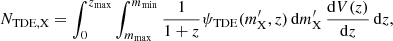
We first expressed the luminosity function, ψTDE, as a function of BH mass, MBH, by multiplying the BH mass function, ϕBH, and the TDE occurrence rate, Γ. We employed a local BH mass function derived from early-type galaxies within 30 Mpc (Gallo & Sesana 2019; Wong et al. 2022),
![Mathematical equation: $$ \begin{aligned} \log _{10}\left(\frac{\phi _{\rm BH}}{\mathrm{Mpc}^{3}\,\mathrm{M}_\odot }\right) &= -9.82 -1.10\log _{10}\left(\frac{M_{\rm BH}}{10^{7}\,\mathrm{M}_\odot }\right)\nonumber \\&\quad - \left[\frac{M_{\rm BH}}{128 \times 10^{7}\,\mathrm{M}_\odot }\right]^{\left(\frac{1}{\ln (10)}\right)}, \end{aligned} $$](/articles/aa/full_html/2024/10/aa49481-24/aa49481-24-eq2.gif) (2)
(2)
which gives the number of BHs per volume for a given MBH range. We assumed that ϕBH does not evolve with redshift. This BH mass function is shown in Figure 1. One can derive a redshift dependent BH mass function by combining a galaxy mass function and a galaxy-BH scaling relation. However, galaxy scaling relations may break down near the low-mass end, and the occupation fraction of BHs in high-z dwarf galaxies is uncertain. Since low-mass SMBHs would create the majority of TDEs, we employed the BH mass function that takes into account the occupation fraction although it is valid only for the local universe. This is still a reasonable approach given that this BH mass function was constructed in a way to account for the various uncertainties inherent to the scaling relation. This function was the best fit to the occupation fraction of over 300 local galaxies observed by the Chandra X-ray Observatory. We will explore the dependence of the lensed TDE rates on the redshift evolution of the BH mass function in our future work.
 |
Fig. 1. BH mass function ϕBH for the range of 105–108 M⊙. |
We took the TDE occurrence rate, Γ, from Pfister et al. (2020),
 (3)
(3)
which yields for a given BH mass the number of TDEs per galaxy per year. This relation was obtained through constructing a mock catalog of galaxies that were based on empirical relations. For each central BH, there was an assumed loss-cone region around it from which the authors estimated the TDE occurrence rate given the surrounding stellar population. This rate is in agreement with current observed TDE rates. This TDE rate per galaxy is also valid within the local universe and assumed to not evolve with redshift. We selected this TDE rate because of its agreement with the observed TDE rate and due to the upper limit on the BH mass, above which stars are expected to be swallowed whole rather than disrupted.
Then, assuming each galaxy harbors one massive BH at its center, we wrote ψTDE(MBH) as,
![Mathematical equation: $$ \begin{aligned} \psi _{\rm TDE}\left(M_{\rm BH}\right) =\phi _{\rm BH}\Gamma = 10^{-13.22} \left(\frac{M_{\rm BH}}{10^{6}\,\mathrm{M}_\odot }\right)^{-1.24}10^{ -\left[\frac{M_{\rm BH}}{128\times 10^{7}\,\mathrm{M}_\odot }\right]^{\left(\frac{1}{\ln (10)}\right)}}. \end{aligned} $$](/articles/aa/full_html/2024/10/aa49481-24/aa49481-24-eq4.gif) (4)
(4)
From Eq. (4), ψTDE dMBH gives the number of TDEs per year per volume within a BH mass range of MBH to MBH + dMBH. We considered the range of MBH within 105 M⊙ and 108 M⊙ based on current observational constraints such as, e.g., the TDEs from ZTF (Yao et al. 2023). Above the upper limit of ∼108 M⊙ in the BH mass, stars are swallowed whole by the central BH rather than being tidally disrupted.
2.3. Conversion from ψTDE(MBH) to ψTDE(L)
We then found the expression for ψTDE(L) from the relation ψTDE(L) = ψTDE(MBH(L)) dMBH/dL. To do this, we considered two different TDE luminosity expressions, which allowed us to assess how the differing assumptions in turn altered the detection rate. The first, which we denoted as L1, is an observationally driven upper limit that about 1% of the rest mass energy of the stellar fallback material produced in a disruption of 0.1 M⊙ main-sequence star turns into radiation with an efficiency of η = 0.01 (Thomsen et al. 2022),
 (5)
(5)
where Ṁfb is the mass fallback rate of the most bound debris, and c is the speed of light1. Using the expression of Ṁfb (see Eq. (16) in Ryu et al. 2020a), we obtained,
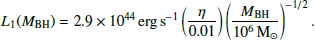 (6)
(6)
The second luminosity, denoted L2, is driven by self-crossing shocks between debris streams (Ryu et al. 2020b),
 (7)
(7)
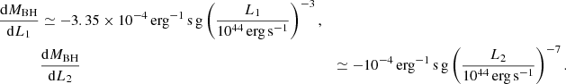
where the apocenter distance of the most bound debris a is estimated assuming a 1 M⊙ star. (Ryu et al. 2020a) corrected the luminosity using a correction factor that incorporates relativistic effects and realistic stellar internal structure. In this work, we only took the correction for the internal structure and neglected the term for relativistic effects. It is because this is only relevant at higher MBH, which constitutes an insignificant fraction of the detected population. In Figure 2, the luminosity models are shown for the BH mass range that we consider, and these are plotted with optically observed TDEs to show how they correspond with observed data. As we later mention in Sect. 2.5, we limit the luminosity for L1 so as to produce more realistic rates, so we show the Eddington limited L1 (solid blue) in this Figure. This Eddington limited L1 model is used throughout the rest of this work; the dotted blue line for the L1 without an Eddington limit is shown for reference and not used for computing detection rates.
 |
Fig. 2. Two luminosities of TDEs, L1 (Eq. (6), Thomsen et al. 2022) and L2 (Eq. (7), Ryu et al. 2020b) as a function of MBH overlaid with observed optical TDEs using gray dots and error bars (see Table A.1 in Wong et al. 2022 and Table 1 in Ryu et al. 2020b, and references therein). The dotted blue line conveys L1 as given by Eq. (6), whereas the solid blue line show the Eddington limited L1. |
Using Eqs. (6) and (7), we computed dMBH/dL for both L1 and L2,
 (8)
(8)
So we found an expression for ψTDE(L) using Eqs. (6) and (8) for L1 and Eqs. (7) and (9) for L2. Note that dMBH/dL has a negative sign because L is anti-correlated with MBH (see Eqs. (6) and (7)). This also means that the negative sign of dMBH/dL will be canceled by integrating over L from a larger L to a smaller L, corresponding to integrating from the lower bound of MBH to the upper bound, giving positive Ψunlensed.
2.4. Conversion from ψTDE(L) to ψTDE(mX, z)
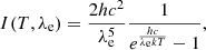
We needed to convert ψTDE(L) into ψTDE(mX, z) using the relation ψTDE(mX, z) = ψTDE(L(mX, z)) dL/dmX. To do this, we needed to find an expression of the magnitude mX as a function of L. We assumed a blackbody spectrum with a constant temperature T, giving the spectral intensities, in units of power per solid angle per area per wavelength, in the source frame as,
 (9)
(9)
where h is the Planck constant, k the Boltzmann constant, and λe the emitted wavelength. It follows that the observed flux is,
 (10)
(10)
where DL is the luminosity distance of the source, λo the observed wavelength, λo = (1 + z)λe, z the source redshift, and σ the Stefan–Boltzmann constant. Note that I(T, λo) in Eq. (11) is the same as Eq. (10) but in terms of observed wavelength.
As driven by observations, we assumed that the TDEs have a relatively constant temperature at peak luminosity across the population with a temperature ranging from (1 − 5)×104 K (e.g., Gezari 2021). Figure 3 shows the observed flux for five different temperatures within our considered temperature range. A typical luminosity of L = 1044 erg s−1 is chosen to convey these flux trends for multiple temperatures, and the redshifts correspond to median source redshifts for detectable unlensed TDEs by LSST and ZTF which we will show in Sect. 2.5. We indicated the wavelength range of each band for both surveys using different colors. The observed wavelength at the peak of the flux λo, peak follows the Wien’s displacement law, λo, peak ∝(1 + z)/T. For LSST, the flux peaks fall at an observed wavelength of λo, peak = 5799, 2899, 1933, 1449 and 1160 Å for T = 1, 2, 3, 4 and 5 × 10⁴ K, respectively. For ZTF, the fluxes peak at λo, peak = 3480, 1740, 1160, 870 and 696 Å taken over the same temperature range as LSST.
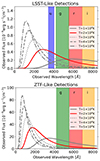 |
Fig. 3. Observed flux for a TDE with L = 1044 erg s−1 at T = 1, 2, 3, 4 and 5 × 10⁴ K assuming typical redshifts given our unlensed computations for LSST and ZTF which are z = 1.0 and z = 0.2, respectively. |
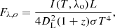
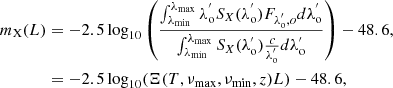
We used the observed flux to calculate the apparent magnitude mX for a particular filter X (X = u, g, r, and i bands) within the filter wavelength limits λmin to λmax (Bessell & Murphy 2012).
 (11)
(11)
where SX(λ) is the transmission function for filter X, and Ξ(T, νmax, νmin, z) is the collection of all terms from the integration except L so as to simply show the relation between magnitude and luminosity. We provided the apparent magnitude in terms of frequency as performing the integration over frequency allowed us to obtain an analytic expression for the apparent magnitude. As shown in Figure 1 of Huber et al. (2021), the transmission functions are well approximated by top-hat functions for the different wavelength ranges. We assumed a top-hat function for these filter functions with the wavelength ranges approximated at λu = 3450 − 4050 Å, λg = 4220 − 5550 Å, λr = 5540 − 6910 Å and λi = 6920 − 8180 Å. These approximations are determined by fitting the LSST filter functions, but these are also reasonable approximations for the ZTF filters (see Figure 2 in Bellm et al. 2018). Now, Ξ can be expressed as
![Mathematical equation: $$ \begin{aligned} \Xi (T, \nu _{\rm max}, \nu _{\rm min},z) &=\left[\frac{(1 + z )}{4D_{L}^{2}\sigma T^{4}c^{2}h^{2}} \right]\left[\ln \left(\nu \right) \Big |_{\nu _{\rm min}}^{\nu _{\rm max}}\right]^{-1}\nonumber \\&\quad \times \Big [ 2hkT \nu (1+z) \left(h \nu (1+z) \ln \left[1 - e^{\frac{-h \nu (1+z)}{kT}} \right]\right.\nonumber \\&\quad \left.- 2kT \mathrm{Li}_{2}\left(e^{\frac{-h \nu (1+z)}{kT}}\right)\right)\nonumber \\&\quad - 4(kT)^{3}\mathrm{Li}_{3}\left(e^{\frac{-h \nu (1+z)}{kT}}\right)\Big |_{\nu _{\rm min}}^{\nu _{\rm max}}\Big ], \end{aligned} $$](/articles/aa/full_html/2024/10/aa49481-24/aa49481-24-eq12.gif) (12)
(12)
where Lis(z) is a polylogarithm of order s and argument z.
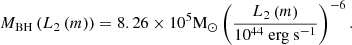
Figure 4 shows how the apparent magnitude changes with temperature, at z = 1.0. For i band, as temperature increases, the apparent magnitude becomes progressively fainter. Whereas the trend is initially the opposite for the other three bands, the apparent magnitude becomes brighter before dimming, yet the u and g bands still remain brighter than the other two bands for T > 2.2 × 10⁴ K. As apparent magnitude directly depends on the observed flux, these trends are a result of the peak of the observed flux moving out of the i and r bands and into the bands corresponding to shorter wavelengths, u and g, for an increasing temperature as seen in Figure 3. Given these magnitude trends for LSST-like limiting magnitudes, we can expect that at the lowest temperature, the i and r bands will have the highest detections. In contrast, the mid-range to higher temperatures will result in g band having the highest detections; u band, while bright at these temperatures as well, is less sensitive which will inhibit its detections.
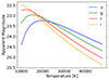 |
Fig. 4. Apparent magnitudes for u, g, r, and i bands as a function of temperature at a redshift of z = 1.0 and assuming L = 1044 erg s−1. |
With the expression for the apparent magnitude, we determined dL/dmX. Since Ξ does not depend on L, the derivative is simply,
 (13)
(13)
The expression for ψTDE(m, z) can then be found using Eqs. (12), (13), and (14) for L1 and L2 (See Appendix A for full expression). The resulting luminosity functions for L1 and L2 are shown in Figure 5. Finally, using ψTDE(m), zmax, mmin and mmax, we determined the unlensed TDE detection rates by computing Eq. (1) for a given band.
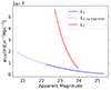 |
Fig. 5. Luminosity function in terms of magnitude for L1 (the L1 without an Eddington limit is given by the dotted blue line while the Eddington limited L1 is shown in solid blue) and L2 at a redshift of z = 1.0 where the apparent magnitude range shown corresponds to the MBH range of 105 − 108 M⊙ considered throughout this paper. |
2.5. Unlensed rates of TDEs
We computed the unlensed detection rates for a range of magnitude cutoffs. This allows us to generalize the unlensed detection rates to more than LSST and ZTF by estimating these detection rates for surveys with any given survey area and magnitude limit. The TDE magnitudes that we have considered in Sect. 2.4 are the brightness at the peak of the TDE light curve. Therefore, we consider magnitude cutoffs brighter than the limiting magnitudes of surveys in order to obtain more detections along the TDE light curve near their peak brightness to allow these TDEs to be properly detected and classified. We will refer to these cutoff magnitudes at peak as mlim, peak. Additionally, to have more realistic luminosities in the L1 regime, we set an upper bound on L1 to be the Eddington luminosity for the given MBH.
Throughout this work, we used three observational models to determine detection rates made by LSST and ZTF given different survey limiting magnitudes. The first LSST model, denoted LSST1, defined the magnitude cutoff as a magnitude value of 0.7 less than the LSST magnitude band limit, mlim, survey (Oguri & Marshall 2010). The choice of a peak TDE brightness 0.7 magnitudes brighter than the survey limit is to allow for multiple detections near the peak of the light curve so as to detect and classify the source as a TDE. TDEs typically drop a magnitude from their peak brightness over a few tens of days, so requiring the peak to be 0.7 brighter than the survey’s limiting magnitude would allow for multiple detections given the cadence of LSST. We applied the same cutoff criterion to the ZTF limit as in LSST1. The mlim, survey values for LSST and ZTF are given by (u, g, r, i) = (23.3, 24.7, 24.3, 23.7) (e.g., Huber et al. 2021; Lochner et al. 2022) and (g, r, i) = (20.8, 20.6, 19.9) (Bellm et al. 2018), respectively, where ZTF does not observe in the u band. We also considered an additional LSST model, LSST2, which defined the cutoff as 2.0 magnitudes less than that of the LSST mlim, survey (Bricman & Gomboc 2020). Similar to our choice of the LSST1 peak magnitude, requiring the peak magnitude to be 2.0 brighter than the survey’s limiting magnitude is a more conservative approach to ensuring that a sufficient number of detections are obtained to classify the source as a TDE. In this model, a TDE would be observable for a significantly longer amount of time, on the order of a hundred days or more. We summarize the three magnitude cutoffs we utilized in Table 1.
Three observational magnitude cutoffs used for computing the unlensed TDE detection rates given the survey limiting magnitudes (e.g., Bellm et al. 2018; Huber et al. 2021; Lochner et al. 2022). Here, X = u, g, r, and i.
In Figure 6, we show the annual unlensed detection rates for L1 and L2 at a temperature of T = 2 × 10⁴ K to illustrate the unlensed detection rates assuming a generic mlim, peak, but as we will soon see this temperature matches well with observations. We also provide the LSST1 and ZTF detection regions to indicate where these magnitude ranges fall within the curves. While the models of the detection regions that we indicate are motivated by previous studies (Oguri & Marshall 2010; Bricman & Gomboc 2020), one can estimate the rate with any magnitude cut using Figure 6.
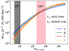 |
Fig. 6. Annual unlensed TDE detection rates as a function of the peak brightness, mlim, peak, at T = 2 × 10⁴ K for L1 in solid lines and for L2 shown in dotted lines. The limiting magnitudes for the different filters of ZTF and LSST surveys are within the gray and pink shaded areas, respectively. These limiting magnitudes are 0.7 brighter than the survey limiting magnitude mlim, survey (i.e., mlim, peak = mlim, survey − 0.7), denoted by LSST1, in order for TDEs to have multiple detections near their peak brightness above the limit mlim, survey. |
In Figure 6, we see that as mlim, peak increases, the annual unlensed detection rates for both luminosities increase correspondingly as observing at these fainter magnitudes enables the detections of observations at further redshifts. L1 and L2 have comparable detection rates with L2 producing slightly larger rates in general. We are also able to observe how the more successful band changes with the peak magnitude. For a brighter mlim, peak, the u and g bands produce the greater number of detections, but both L1 and L2 experience a crossing at mlim, peak ≃ 23.3. At fainter magnitudes, the i and r bands produce more detections which is a result of these sources being at further distances, and this implies that their observed fluxes would be redshifted. The relation between an increasing redshift and the observed flux is seen in Figure 3 when comparing the ZTF-like detections, at z = 0.2, and the LSST-like detections, at z = 1.0. At all temperatures, when the source is at a further redshift, this peak of the observed flux is pushed to longer wavelengths which indicates that at such larger redshifts we expect i and r bands to dominate the detections.
We also present the unlensed detection rates as a function of MBH for the LSST1 survey in Figure 7. We find that the lower BH masses dominate the detections and that the detections decrease with BH mass. The distribution shape differs notably between L1 and L2 for lower BH masses because the luminosity of L1 is Eddington limited, and by Eq. (6) this significantly impacts the lower masses. Thus, limiting L1 luminosity flattens off the distribution at lower masses, especially for MBH < 106 M⊙.
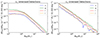 |
Fig. 7. Annual unlensed L1 (left panel) and L2 (right panel) detection rates for u, g, r and i bands as a function of MBH assuming LSST1 limiting magnitudes. |
Next, we calculate the unlensed TDE detection rates using Eq. (1) as a function of temperature for the models referenced previously, LSST1, LSST2 and ZTF, given in Tables 2 and 3. In Figures 8 and 9, we show that LSST1 results in higher detections than that of ZTF since it employs fainter peak magnitude limits. We can see that the g band detection rates are generally higher than those for other bands within the temperature range considered, independent of the assumption for the luminosity. Figure 8 shows that the L1g band detection rate for LSST1 is 1.4 × 10⁴ at T = 1 × 10⁴ K which decreases to 3.6 × 10³ at T = 5 × 10⁴ K. Whereas, ZTF’s largest detection rate is 8.3 × 10² for L1g band at T = 1 × 10⁴ K before the rates proceed to decline. For L1, the LSST1 detection rates at T = 1 × 10⁴ K are 1.5 × 10⁴, 1.3 × 10⁴ and 1.4 × 10⁴ for r, i, and g bands, respectively, and these detection rates are 1.9 × 10⁴, 1.7 × 10⁴ and 1.6 × 10⁴ for L2. As temperature increases, g band results in the highest detections. The g band detections peak at 2 × 10⁴ K for both luminosities with a detection rate of 1.8 × 10⁴ for L1 and 2.3 × 10⁴ for L2. Then, as the temperature increases further, the detections decrease because the flux peak shifts more into the ultraviolet range as seen in Figure 3. It then follows that, as the more conservative LSST approach, LSST2 detects fewer TDEs than LSST1 but still greater than that of ZTF.
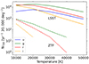 |
Fig. 8. L1 annual TDE detection rate with varying temperatures for LSST1, shown in solid lines, and ZTF, shown in dashed lines. |
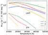 |
Fig. 9. L2 annual TDE detection rate with varying temperatures for LSST1, shown in solid lines, and ZTF, shown in dashed lines. |
In Figures 10 and 11, we present the number of unlensed TDE detections per band (given by the height of the histograms) and the hierarchy of the four bands we consider for the unlensed L1 and L2 detections, respectively, in the range of T = (1 − 5) × 104 K assuming LSST1 magnitude cutoffs. We obtain this hierarchy by computing how many detections within a particular band are also detected in the remaining three bands, and this allows us to determine the overlap of detections across the bands. For L1 in Figure 10, we see that there is a complete hierarchy for T = (3 − 5)×104 K; at these temperatures, we find that g ⊃ r ⊃ u ⊃ i where a ⊃ b means a encompasses b. For the remaining two temperatures, there are partial overlaps between bands rather than each successive band’s detections being encompassed in those of the previous band. For example, at T = 1 × 10⁴ K, the green g histogram has a section that is outside both the r and i histograms, so this indicates that there are detections in g band that are not seen in either r or i bands. There is a similar occurrence for the u band in comparison to the i band at T = 2 × 10⁴ K. Partial overlappings are likely due to a TDE’s magnitude being fainter than a band’s mlim, peak at LSST1 magnitude cutoffs. As an example, we show in Appendix B the relation between mr and mg at two different temperatures for three constant luminosity cases, and it can be seen that some luminosities will be detected in r and not in g and vice versa depending on the particular L and T. These relations exist across all bands and can help to explain why TDE detections may be missed in the other bands.
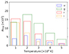 |
Fig. 10. Number and hierarchy of unlensed L1 detections for each of the four bands across the five temperatures we consider given LSST1 magnitude cutoffs. The band that results in the most detections for each temperature is the tallest rectangle (i.e., the r band for T = 1 × 10⁴ K and g band for all other temperatures) where the height of the rectangle indicates the number of detections, and a rectangle contained within another implies that a detection in that band is also detected in the encompassing band. For instance, in the T = 3 × 10⁴ K case, the yellow rectangle for i band is contained entirely within the green, red and blue rectangles for g, r and u bands, respectively. This indicates that all i band detections are also detected within g, r and u bands. The partial overlapping for T = 1 × 10⁴ K (g and i) and 2 × 10⁴ K (u and i) means those detections do not establish a full hierarchy. Note that the width and the degree of overlap of the rectangles do not convey any significant meaning. |
For L2 in Figure 11, we observe that there is a complete hierarchy for T ≥ 2 × 10⁴ K. For example, for T = 2 × 10⁴ K, g ⊃ r ⊃ i ⊃ u. For the T = 1 × 10⁴ K case, we observe that r band is the dominating filter that encompasses all other detections. However, while i band detects more TDEs than g band, i band does not detect all of the g band TDEs, but despite this all of the u band detections are also seen in both g and i which is why the blue u rectangle is contained entirely within the g and i band overlapping regions. However, we note that the number of g band detections missed in i band is approximately on the order of the statistical fluctuations. The number of detections in each of the bands and the overlap between bands are also tabulated in Appendix B.
Our unlensed detection rates are generally higher by roughly two or three to 20 than the ZTF detection rates in the r and g bands, which are on the order of 10–20 TDEs annually (see, e.g., Yao et al. 2023) with T ≃ (2 − 3)×104 K (e.g., Hammerstein et al. 2023). We attribute this difference to a possible stronger contribution of low-mass MBH to the rate in our estimates (especially for L2) and the incompleteness of observations. While the inference of MBH from observations is highly dependent on the emission models, the inferred MBH for ZTF TDEs tends to be greater than 106 M⊙ (e.g., Hammerstein et al. 2023). We also find that our LSST detection rates are consistent with other studies. Our conservative LSST2 model was following Bricman & Gomboc (2020), and we find rates consistent with their estimates of 35 000–80 000 TDEs observed throughout the lifetime of LSST, especially for that of T = 2 × 10⁴ K which we will take as our fiducial temperature for the remainder of this work.
3. Rates of lensed TDEs
3.1. Overview of method
We utilized the code developed by Oguri & Marshall (2010) that was used to produce mock catalogs for strongly lensed supernovae and quasars. We implemented the rate calculation of unlensed TDEs into the code to produce similar mock catalogs for strongly lensed TDEs. This method constructed a source table given a magnitude range, redshift range and the luminosity function of the source that was obtained in Sect. 2.4 and shown in Figure 5. This source table was obtained through gridding the magnitude and redshift range provided and numerically computing the number of TDEs at each grid point. Then, we determined which of these TDEs would be strongly lensed and were outputted into a catalog of lensed TDEs. Here, we set the magnitude to span the range from a sufficiently bright magnitude (m = 15.0) to a magnitude of m = 27.0. From the output catalog of the lensed TDEs, we subsequently applied brighter limiting magnitude cutoffs such that we obtained the detection rates for any cadenced imaging survey with single-epoch limiting magnitude brighter than mlim, peak = 27.0. We probed from the local universe to a sufficiently high redshift of z = 6.8 for L1 and z = 5.5 for L2 where these values were chosen to be greater than the largest zmax across all bands for both cases to avoid missing any detections by not probing to far enough distances.
In this method, the lenses were taken to be elliptical galaxies with mass distributions described by the singular isothermal ellipsoid. The environment effects of each lens were characterized by an external shear. While Oguri & Marshall (2010) assumed no redshift evolution for the velocity dispersion function, in this paper the lenses were distributed such that their velocity dispersion functions evolved with redshift as defined by Eq. (11) in Oguri (2018). As discussed in Oguri (2018), varying the velocity dispersions of the lenses can influence the lensing probability by up to a factor of two, and it would similarly affect the magnifications for some sources experiencing a larger magnification. While the choice of a velocity dispersion that is constant with redshift holds for low redshift galaxies Bezanson et al. (2011), since we set a maximum redshift of z = 2.0 for the lenses, incorporating a velocity dispersion that evolves with redshift is more applicable. The lensing probability of a given source was computed by integrating over image separation and source redshift for a given TDE (see Eq. (5) in Oguri & Marshall 2010), and from this the total number of strong lenses can be determined. The lensing for these sources was then simulated. For a strongly lensed double system to be detected, we required that both images must have a magnitude brighter than mlim, peak; for a quadruple system, we required that three images must be brighter than mlim, peak. The choice of the third brightest image is due to the fact that this image tends to appear first, and it is often further from the brightest image which allows it to be more easily identified as a strongly lensed system. We then obtained the image separation, magnitude of the lensed third brightest image (or fainter image for double systems), redshifts of the lens and TDE as well as the locations and magnifications of all images within the lensed systems.
We used the TDE luminosity function in terms of magnitude, ψTDE(m, z), to construct the TDE source table. To reduce statistical noise (i.e., statistical fluctuations given the typically low rates of lensed TDEs) and obtain a sufficiently large number of mock lenses to produce distributions, we oversampled each simulation run by a factor of 1000 and then renormalized the output number of lenses by this factor. We limited the L1 luminosity to the Eddington luminosity, as for the unlensed case. The luminosity was then used to compute the unlensed TDE magnitude and together with the magnification it was used to compute the lensed magnitude.
3.2. Results
We computed the strongly lensed TDE detection rates for L1 and L2 assuming a constant temperature of 2 × 10⁴ K.
In a strongly lensed system, the image separation must be large enough to be resolved, so we retained only detections with image separations within the range of 0.5″–4″. The choice of the image separation cut off at 4″ is because we focus on galaxy-scale lenses in this study whose image separations are typically ≲4″ (larger image separations would correspond to galaxy groups or galaxy clusters as lenses). We show the strongly lensed detection rates per effective year for various bands assuming a variable lensed peak magnitude, mlim, peak, for each of the L1 and L2 luminosity functions.
3.2.1. Rates
As mlim, peak increases, the strongly lensed detection rates increase as well given that we are able to detect fainter and fainter lensed TDEs which, in turn, implies that we are probing at further and further distances. The lensed detection rates per effective year of observation for each of the four bands along with the LSST1 and ZTF magnitude cutoffs are shown in Figure 12 for L1 (left panel) and L2 (right panel). These rates assume a survey area of 20 000 deg2, and since the area of ZTF is larger than LSST, these rates become a lower limit estimate for ZTF. From this, it is unlikely that ZTF will detect a strongly lensed TDE. However, the results are more promising for that of LSST. Since these detection rates are for a single effective year of observation, these results must be multiplied by the effective duration of LSST to determine the detection rates for the entirety of LSST. The lensed detection rates for the duration of LSST for L1 and L2 are shown in Table 4 assuming an effective duration of 4.5 years which is typical for the LSST baseline observing strategy (Huber et al. 2019; Lochner et al. 2022).
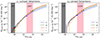 |
Fig. 12. Strongly lensed L1 (left panel) and L2 (right panel) detection rates per effective year of observation for u, g, r and i bands assuming a variable peak magnitude, mlim, peak. The mlim, peak ranges for ZTF and LSST1 assuming a survey area of 20 000 deg2 are shown in gray and pink, respectively. The LSST1 mlim, peak values for each of the four bands are overlaid along the curves in stars, and the ZTF mlim, peak values for g, r and i are overlaid along the curves in diamonds. |
Lensed TDE detection rates for L1 and L2 using the LSST1 magnitude cutoffs at T = 2 × 10⁴ K for the entire duration of LSST assuming a typical effective duration of 4.5 years. These lens systems have multiple TDE images separated by > 0.5″.
Specifically, for L1, the lensed detection rates per effective year of observation are (u, g, r, i) = (11, 17, 22, 27) at a lensed magnitude of mlim, peak = 27.0. The lensed rates for L2 are (u, g, r, i) = (13, 20, 28, 33). The lensed LSST detection rates for L1 and L2 show that g band will be the most successful (as shown by the star symbols in Figure 12). At further magnitudes, the trend resembles that of the unlensed case with the i band resulting in the highest detections for both L1 and L2 as shown in Figure 12. Thus, at these fainter peak magnitudes, i and r bands are expected to produce the most strongly lensed detections for both luminosities. With mlim, peak = 27.0 for an effective duration of 4.5 years, L2 is expected to detect the most lensed TDEs within the i band; given LSST1 cutoffs, the r band is expected to detect approximately 5 more lensed TDEs than i band, but at this further mlim, peak = 27.0, i band is anticipated to detect 23 more lensed TDEs than r band. L1 is projected to detect on the order of 50 more strongly lensed TDEs in i band than in g band at mlim, peak = 27.0.
Given the lensed detection rates, we can further investigate the occurrence of a lensed detection by determining the ratio of lensed to unlensed detections. These ratios assuming an LSST1 survey for all bands of L1 are (u, g, r, i) = (4.2, 11, 8.3, 9.9) × 10−5, and similarly for L2 these ratios are (u, g, r, i) = (4.2, 11, 11, 9.2) × 10−5. Thus, L1 and L2 produce similar relative ratios of lensed to unlensed events, especially for u and g bands. Additionally, these ratios indicate that for every 104 unlensed TDE detections, we may detect ∼1 lensed event. Although the scaling factor would depend on several assumptions, it can serve as a rough but useful guide to estimate the lensed rates from the unlensed rates without detailed calculations.
3.2.2. Lens properties
The distributions showing the lensing properties are constructed using the full catalog that was oversampled by a factor of 1000 for each band, and the resulting figures are then normalized by this factor to show the lensed detection rates for a single effective year of observation.
In Figure 13, we show the properties of the L2 lensing systems for u, g, r and i bands that would still be detected after applying LSST1 magnitude cuts. These panels indicate that g and r bands result in greater detections than the other bands, but we can also see that the properties of the systems detected by these two bands are very similar. The source redshift corresponding to the peak of the u band distribution is at zs = 1.0, but in the top middle panel we observe the peak shifting to further redshifts, as in the unlensed case, such that the peaks fall at zs = 1.2 and zs = 1.4 for g and r bands, respectively. The image separation distributions are similar across all bands; the majority of strongly lensed systems have smaller image separations with θsep ≲ 1″, and as the image separations increase further the distributions fall off as systems with larger separations are more unlikely. The lens velocity dispersion distributions are also similar across all four bands.
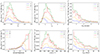 |
Fig. 13. Distributions of the lensing properties of the strongly lensed L2 systems from detections in each of the u, g, r and i bands after applying image separation cuts and LSST1 magnitude cuts. Top panels from left to right: lens galaxy redshift zl, TDE redshift zs, and image separation θsep. Bottom panels from left to right: lensed magnitude (magnitude of the fainter image in a double system or the third brightest image in a quadruple system), stellar velocity dispersion σ of the lens galaxy, and time delays tdelay of all images in the lensed systems. |
The g band lensing properties for L1 and L2 are presented together in Figure 14 to compare the results from these two luminosity models. We find that the distributions for these models are very comparable with the primary difference being that L2 produces higher rates in general. We do not see a larger difference in the lensed magnitude panel, despite the L1 luminosity spanning a larger magnitude range, because we have limited L1 based on the Eddingtion luminosity.
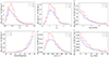 |
Fig. 14. Distributions of the lensing properties of the strongly lensed L1 and L2 systems for g band after applying image separation cuts. These distributions assume LSST1 magnitude cuts, and the panels are arranged in the same way as in Figure 13. In general, the shapes of the distributions of the lensing properties are similar between L1 and L2. |
4. Discussions
In this work, we employ a BH mass function and a TDE rate per galaxy that are valid for the local universe, and we assume that they do not evolve with redshift. As seen in the lensed source redshift distribution in Sect. 3.2.2, the peak of the L2 source redshift distribution for u band is at zs = 1.0, and all of the other bands peak at an even higher redshift. Thus, it would be useful to consider other BH mass functions and TDE occurrence rates that would be more relevant at these redshifts as these could affect the rates, which we will investigate in the future.
Additionally, we assumed a constant temperature for the TDEs. While this is observationally motivated, there is a theoretical temperature dependence for L2 that was not included in this study. This would be an important path for future work to assess how this temperature dependence influences both the unlensed and strongly lensed detection rates.
In general, we observe that, given the LSST1 magnitude cutoff, the L2i and u strongly lensed detections peak at a source redshift comparable to that of lensed supernovae which peak at zs ≲ 1 (Oguri & Marshall 2010; Wojtak et al. 2019) while the g and r bands peak at slightly higher redshifts, and this also applies for L1. Thus, given the detection band, strongly lensed TDEs are expected to be detected at redshifts ∼0.5 higher than that of lensed supernovae. As shown in both Figures 13 and 14, the image separation θsep is peaking toward the lower values for L1 and L2. If we were to retain lensed detections with θsep < 0.5″, we would subsequently obtain more strongly lensed systems. However, many of these systems would likely be unresolved by ground-based imaging surveys such as LSST. Nonetheless, there are methods to find such unresolved systems (e.g., Geiger & Schneider 1996; Bag et al. 2022), so it is useful to note the abundance of lensed systems within this region of θsep. We provide these full image separation distributions including detections with θsep < 0.5″ in Appendix C.
Recently, Chen et al. (2024) estimated the detection rates of strongly lensed TDEs by computing the probability of strong lensing (also known as the “lensing optical depth”) of TDE light curves. They assumed that TDEs are powered by super-Eddington winds generated from an accretion disk that forms after the debris promptly circularizes (Strubbe & Quataert 2009; Lodato & Rossi 2011), which differs from our luminosity models. Despite differences in the assumptions for the luminosity function and the methodology of lensing calculations, our estimates for the lensed TDE detection rates by LSST are quite similar to theirs in the case where stars are tidally and fully destroyed at the largest possible distances from the BH. However, their estimates are very sensitive to the assumption for the distance at which stars are destroyed, directly affecting the luminosity of TDEs, whereas our estimates have a relatively weak dependence on the assumptions for the luminosity. In addition, Chen et al. (2024) considered all lensed TDEs with lensed image separations θsep above 0.1″, which provide higher lensed TDE rates compared to our θsep > 0.5″ limit. In Appendix C, we show also our lensed TDE rates and properties where we drop the 0.5″ criterion and consider all possible image separations. The resulting rates of lensed TDEs per year from their and our independent analyses further corroborates the bright prospect of detecting lensed TDEs in the era of LSST.
5. Summary
In this paper, we present the estimated unlensed TDE detection rates for three observational survey magnitude cutoffs for two TDE luminosity models, L1 and L2, at five distinct temperatures. We show how the unlensed detection rates change for both luminosities with mlim, peak and temperature. We also estimate the strongly lensed TDE detection rates for one of the LSST detection thresholds at the chosen temperature that best corresponds with current TDE observations, and we similarly show how these lensed detection rates change with mlim, peak.
We find that L1 and L2 produce comparable unlensed detection rates. As mlim, peak increases, the detection rates similarly increase as this means that the survey is probing at further depths and is then capable of detecting more TDEs. At lower magnitude cutoffs, the u and g bands result in the higher detections, but, as the magnitude cutoff increases, the TDEs are at further redshifts in general which enables the i and r bands to produce more detections which is well shown in Figure 6. We observe how the LSST1 and ZTF survey detections change with temperature; we find that the unlensed L1 and L2 LSST1 detections peak at T = 2 × 10⁴ K before decreasing, and the ZTF detections all decrease with temperature. We find that, for both L1 and L2, low-mass BHs (MBH ≲ 106 M⊙) contribute the most to the rates, resulting in an overestimate of the ZTF detection rates by about an order of magnitude.
A close investigation for the overlap of unlensed detections across the four bands shows that the g band will yield the highest number of TDEs at T ≥ 2 × 10⁴ K, while r band will yield the highest number at T = 1 × 10⁴ K. However, for L1 with T = 1 × 10⁴ K, the g band may still miss some detections from some of the other remaining bands. To maximize the number of TDE detections, we advocate for using the combination of g, r and i bands in LSST-like surveys, with g and r bands being the primary bands; if observing resources are limited, then we advocate for prioritizing the four bands in the following order: g, r, i and then u.
Similar to the unlensed TDEs, we find that L1 and L2 result in very comparable strongly lensed detection rates with L2 consistently producing higher rates. Assuming the LSST1 cutoff for the peak TDE magnitude given a TDE temperature of T = 2 × 10⁴ K for the entire duration of LSST (4.5 effective years), the estimated strongly lensed detection rates for L1 are (u, g, r, i) = (1.1, 8.7, 7.1, 3.2), and these detection rates for L2 are (u, g, r, i) = (1.5, 11, 9.1, 3.8). These rates indicate that we may detect ∼1 lensed event for every 104 unlensed detections, which is robust against the assumptions for the event luminosity. For L2 with the LSST1 magnitude cutoff, g and r are expected to observe lensed TDEs at higher redshifts than i and u.
Our study shows that strongly lensed TDEs will likely be discovered in the coming years as wide-field imaging surveys such as LSST start operating. This will open a new window to study TDEs via the strong lensing and microlensing effects. We make our catalogs of lensed TDEs available online as part of this publication at Zenodo, which will facilitate future studies of lensed TDEs.
Data availability
The catalogs of unlensed and lensed TDES are available at https://zenodo.org/doi/10.5281/zenodo.12519318
The stellar mass of 0.1 M⊙ and efficiency of η = 0.01 are values that yield a luminosity-mass relation which is compatible with the more luminous TDEs (Figure 2).
Acknowledgments
We are grateful to the anonymous referee for thoughtful and constructive comments and suggestions. We thank S. de Mink for the useful discussions. KS, SHS and SH thank the Max Planck Society for support through the Max Planck Research Group and Max Planck Fellowship for SHS. This project was supported through a Fulbright grant of the German-American Fulbright Commission. This project has received funding from the European Research Council (ERC) under the European Union’s Horizon 2020 research and innovation programme (LENSNOVA: grant agreement No 771776). LD acknowledges the support from the National Natural Science Foundation of China (HKU12122309) and the Hong Kong Research Grants Council (HKU17304821, HKU17314822, HKU27305119). This work was supported by JSPS KAKENHI Grant Numbers JP22H01260, JP22K21349, JP19KK0076.
References
- Arendse, N., Dhawan, S., Sagués Carracedo, A., et al. 2024, MNRAS, 531, 3509 [NASA ADS] [CrossRef] [Google Scholar]
- Bag, S., Shafieloo, A., Liao, K., & Treu, T. 2022, ApJ, 927, 191 [NASA ADS] [CrossRef] [Google Scholar]
- Bellm, E. 2014, in The Third Hot-wiring the Transient Universe Workshop, eds. P. R. Wozniak, M. J. Graham, A. A. Mahabal, & R. Seaman, 27 [Google Scholar]
- Bellm, E. C., Kulkarni, S. R., Graham, M. J., et al. 2018, PASP, 131, 018002 [Google Scholar]
- Bessell, M., & Murphy, S. 2012, PASP, 124, 140 [NASA ADS] [CrossRef] [Google Scholar]
- Bezanson, R., van Dokkum, P. G., Franx, M., et al. 2011, ApJ, 737, L31 [NASA ADS] [CrossRef] [Google Scholar]
- Blackburne, J. A., Kochanek, C. S., Chen, B., Dai, X., & Chartas, G. 2014, ApJ, 789, 125 [NASA ADS] [CrossRef] [Google Scholar]
- Bricman, K., & Gomboc, A. 2020, ApJ, 890, 73 [NASA ADS] [CrossRef] [Google Scholar]
- Chen, Z., Lu, Y., & Chen, Y. 2024, ApJ, 962, 3 [NASA ADS] [CrossRef] [Google Scholar]
- Gallo, E., & Sesana, A. 2019, ApJ, 883, L18 [NASA ADS] [CrossRef] [Google Scholar]
- Geiger, B., & Schneider, P. 1996, MNRAS, 282, 530 [NASA ADS] [Google Scholar]
- Gezari, S. 2021, ARA&A, 59, 21 [NASA ADS] [CrossRef] [Google Scholar]
- Goldstein, D. A., Nugent, P. E., & Goobar, A. 2019, ApJS, 243, 6 [NASA ADS] [CrossRef] [Google Scholar]
- Hammerstein, E., van Velzen, S., Gezari, S., et al. 2023, ApJ, 942, 9 [NASA ADS] [CrossRef] [Google Scholar]
- Hills, J. G. 1988, Nature, 331, 687 [Google Scholar]
- Huber, S., Suyu, S. H., Noebauer, U. M., et al. 2019, A&A, 631, A161 [NASA ADS] [CrossRef] [EDP Sciences] [Google Scholar]
- Huber, S., Suyu, S. H., Noebauer, U. M., et al. 2021, A&A, 646, A110 [NASA ADS] [CrossRef] [EDP Sciences] [Google Scholar]
- Ivezić, Ž., Kahn, S. M., Tyson, J. A., et al. 2019, ApJ, 873, 111 [Google Scholar]
- Kochanek, C. S. 2004, ApJ, 605, 58 [Google Scholar]
- Lochner, M., Scolnic, D., Almoubayyed, H., et al. 2022, ApJS, 259, 58 [NASA ADS] [CrossRef] [Google Scholar]
- Lodato, G., & Rossi, E. M. 2011, MNRAS, 410, 359 [Google Scholar]
- Oguri, M. 2018, MNRAS, 480, 3842 [NASA ADS] [CrossRef] [Google Scholar]
- Oguri, M., & Marshall, P. J. 2010, MNRAS, 405, 2579 [NASA ADS] [Google Scholar]
- Pfister, H., Volonteri, M., Dai, J. L., & Colpi, M. 2020, MNRAS, 497, 2276 [NASA ADS] [CrossRef] [Google Scholar]
- Predehl, P., Andritschke, R., Arefiev, V., et al. 2021, A&A, 647, A1 [EDP Sciences] [Google Scholar]
- Rees, M. J. 1988, Nature, 333, 523 [Google Scholar]
- Ryu, T., Krolik, J., Piran, T., & Noble, S. C. 2020a, ApJ, 904, 98 [NASA ADS] [CrossRef] [Google Scholar]
- Ryu, T., Krolik, J., & Piran, T. 2020b, ApJ, 904, 73 [NASA ADS] [CrossRef] [Google Scholar]
- Schmidt, R. W., & Wambsganss, J. 2010, Gen. Rel. Grav., 42, 2127 [NASA ADS] [CrossRef] [Google Scholar]
- Shvartzvald, Y., Waxman, E., Gal-Yam, A., et al. 2024, ApJ, 964, 74 [NASA ADS] [CrossRef] [Google Scholar]
- Strubbe, L. E., & Quataert, E. 2009, MNRAS, 400, 2070 [NASA ADS] [CrossRef] [Google Scholar]
- Thomsen, L. L., Kwan, T. M., Dai, L., et al. 2022, ApJ, 937, L28 [NASA ADS] [CrossRef] [Google Scholar]
- Wojtak, R., Hjorth, J., & Gall, C. 2019, MNRAS, 487, 3342 [Google Scholar]
- Wong, T. H. T., Pfister, H., & Dai, L. 2022, ApJ, 927, L19 [NASA ADS] [CrossRef] [Google Scholar]
- Yao, Y., Ravi, V., Gezari, S., et al. 2023, ApJ, 955, L6 [NASA ADS] [CrossRef] [Google Scholar]
Appendix A: Full expression for ψTDE(m, z)
The TDE luminosity function in terms of magnitude can be expressed by,
![Mathematical equation: $$ \begin{aligned}&\psi _{\rm TDE}\left(m,z\right) = \psi _{\rm TDE} \left(L_{i}\left(m\right)\right) \frac{\mathrm{d} L_{i}\left(m\right)}{\mathrm{d} m},\nonumber \\&=10^{-13.22} \left(\frac{M_{\rm BH}\left(L_{i}\left(m\right)\right)}{10^{6}\,\mathrm{M}_\odot }\right)^{-1.24}10^{ -\left[\frac{M_{\rm BH}\left(L_{i}\left(m\right)\right)}{128\times 10^{7}\,\mathrm{M}_\odot }\right]^{\left(\frac{1}{\ln (10)}\right)}}\nonumber \\&\times \frac{\mathrm{d} M_\mathrm{BH} \left(L_{i}\left(m\right)\right)}{\mathrm{d} L_{i}\left(m\right)}, \end{aligned} $$](/articles/aa/full_html/2024/10/aa49481-24/aa49481-24-eq14.gif) (A.1)
(A.1)
with i = 1, 2, based on the luminosity model applied, defined as,
 (A.2)
(A.2)
The black hole mass MBH(Li(m)) for L1 and L2 can be obtained from Equations (6) and (7), respectively. These expressions can be given explicitly by,
 (A.3)
(A.3)
 (A.4)
(A.4)
Appendix B: Unlensed magnitude relations
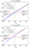 |
Fig. B.1. Unlensed magnitude relationship between r and g bands at T = 2 and 5 × 10⁴ K. Assuming a redshift range of z = 0.1 − 5, three luminosity cases of L = 5 × 1043, 1 × 1044 and 1 × 1045 erg s−1 are shown to represent the luminosity span across L1 and L2, and the mlim, peak values for r and g bands are given by the red and green dashed lines, respectively. |
Figure B.1 shows the relation between the r band magnitude and the g band magnitude for two example cases, one with partial overlappings in detections between bands (top, T = 2 × 10⁴ K) and one with a complete hierarchy in band detections (bottom, T = 5 × 10⁴ K). We take the three constant luminosity values, i.e., L = 5 × 1043 erg s−1, 1044 erg s−1, and 1045 erg s−1, and vary the redshift to examine the magnitude conversion. Since the relation between the two different bands solely depends on the relation between L and m, for given L, the shape of the line is independent of the luminosity models (i.e., L1 and L2). However, each luminosity model covers a different range of L: the two smaller luminosities are covered by the luminosity range for both L1 and L2 while the largest luminosity (1045 erg s−1) is only relevant for L1. For simplicity in this appendix, we do not limit L1 to the Eddington luminosity, as this does not affect the explanation below of the hierarchy different bands for TDE detection.
In the top panel of B.1, all TDEs within the luminosity range of L = 5 × 1043 − 1 × 1044 erg s−1 that are brighter than the g band magnitude are above the r band magnitude (i.e., third quadrant, left side of the green vertical dashed line below the red horizontal dashed line), meaning these TDEs detected in g band would be detected in r band. On the other hand, there are events with L = 1 × 1045 erg s−1 whose magnitudes are still brighter than the mlim, peak, r, but fainter than the mlim, peak, g (fourth quadrant), implying some detections found in r are missed in g. So a full hierarchy between the two bands (g ⊃ r) has been established for the range of luminosity relevant for L2. However, L = 1 × 1045 erg s−1, which is only relevant for L1, reveals the opposite hierarchy (r ⊃ g). Hence, the inhomogeneous hiearchical relation accounts for the partial overlap observed for L1 in Figure 10 and not seen in the L2 hierarchy. Conversely, in the bottom panel, all TDEs within the luminosity range being assessed that are brighter than mlim, peak, r will also be detected in g. For this range of luminosity, there exists a full hierarchy between g and r band detections (g ⊃ r). We observe this trend represented in Figures 10 and 11 by the green box for g being taller than the red r box.
The annual unlensed detections for L1 and L2 for each band at all temperatures are provided in Tables B.1 and B.2. The magnitude of each TDE in the other three bands were computed to determine which bands the TDE would be detected in, and the detection counts in the other bands are listed under the ‘Detected Band’ region of the tables.
Annual unlensed L1 detection rates per band that would be detected in the other three bands for all five temperatures given LSST1 magnitude cuts. The * symbols indicate the rate for the catalog bands.
Same as Table B.1, but for L2.
Appendix C: Full θsep distributions
The full θsep distributions for the lensed TDEs are shown in Figure C.1. These distributions do not require that θsep > 0.5″, so these distributions provide an understanding on the number of systems that would likely be unresolvable by ground-based imaging surveys.
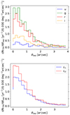 |
Fig. C.1. Lensed TDE image separation distributions assuming LSST1 magnitude cutoffs without the condition that θsep > 0.5″. The top panel shows the distributions for all four bands for L2, and the bottom panel shows the g band distributions for L1 and L2. |
All Tables
Three observational magnitude cutoffs used for computing the unlensed TDE detection rates given the survey limiting magnitudes (e.g., Bellm et al. 2018; Huber et al. 2021; Lochner et al. 2022). Here, X = u, g, r, and i.
Lensed TDE detection rates for L1 and L2 using the LSST1 magnitude cutoffs at T = 2 × 10⁴ K for the entire duration of LSST assuming a typical effective duration of 4.5 years. These lens systems have multiple TDE images separated by > 0.5″.
Annual unlensed L1 detection rates per band that would be detected in the other three bands for all five temperatures given LSST1 magnitude cuts. The * symbols indicate the rate for the catalog bands.
All Figures
|
Fig. 1. BH mass function ϕBH for the range of 105–108 M⊙. |
| In the text | |
|
Fig. 2. Two luminosities of TDEs, L1 (Eq. (6), Thomsen et al. 2022) and L2 (Eq. (7), Ryu et al. 2020b) as a function of MBH overlaid with observed optical TDEs using gray dots and error bars (see Table A.1 in Wong et al. 2022 and Table 1 in Ryu et al. 2020b, and references therein). The dotted blue line conveys L1 as given by Eq. (6), whereas the solid blue line show the Eddington limited L1. |
| In the text | |
|
Fig. 3. Observed flux for a TDE with L = 1044 erg s−1 at T = 1, 2, 3, 4 and 5 × 10⁴ K assuming typical redshifts given our unlensed computations for LSST and ZTF which are z = 1.0 and z = 0.2, respectively. |
| In the text | |
|
Fig. 4. Apparent magnitudes for u, g, r, and i bands as a function of temperature at a redshift of z = 1.0 and assuming L = 1044 erg s−1. |
| In the text | |
|
Fig. 5. Luminosity function in terms of magnitude for L1 (the L1 without an Eddington limit is given by the dotted blue line while the Eddington limited L1 is shown in solid blue) and L2 at a redshift of z = 1.0 where the apparent magnitude range shown corresponds to the MBH range of 105 − 108 M⊙ considered throughout this paper. |
| In the text | |
|
Fig. 6. Annual unlensed TDE detection rates as a function of the peak brightness, mlim, peak, at T = 2 × 10⁴ K for L1 in solid lines and for L2 shown in dotted lines. The limiting magnitudes for the different filters of ZTF and LSST surveys are within the gray and pink shaded areas, respectively. These limiting magnitudes are 0.7 brighter than the survey limiting magnitude mlim, survey (i.e., mlim, peak = mlim, survey − 0.7), denoted by LSST1, in order for TDEs to have multiple detections near their peak brightness above the limit mlim, survey. |
| In the text | |
|
Fig. 7. Annual unlensed L1 (left panel) and L2 (right panel) detection rates for u, g, r and i bands as a function of MBH assuming LSST1 limiting magnitudes. |
| In the text | |
|
Fig. 8. L1 annual TDE detection rate with varying temperatures for LSST1, shown in solid lines, and ZTF, shown in dashed lines. |
| In the text | |
|
Fig. 9. L2 annual TDE detection rate with varying temperatures for LSST1, shown in solid lines, and ZTF, shown in dashed lines. |
| In the text | |
|
Fig. 10. Number and hierarchy of unlensed L1 detections for each of the four bands across the five temperatures we consider given LSST1 magnitude cutoffs. The band that results in the most detections for each temperature is the tallest rectangle (i.e., the r band for T = 1 × 10⁴ K and g band for all other temperatures) where the height of the rectangle indicates the number of detections, and a rectangle contained within another implies that a detection in that band is also detected in the encompassing band. For instance, in the T = 3 × 10⁴ K case, the yellow rectangle for i band is contained entirely within the green, red and blue rectangles for g, r and u bands, respectively. This indicates that all i band detections are also detected within g, r and u bands. The partial overlapping for T = 1 × 10⁴ K (g and i) and 2 × 10⁴ K (u and i) means those detections do not establish a full hierarchy. Note that the width and the degree of overlap of the rectangles do not convey any significant meaning. |
| In the text | |
 |
Fig. 11. Same as Figure 10, but for L2. |
| In the text | |
|
Fig. 12. Strongly lensed L1 (left panel) and L2 (right panel) detection rates per effective year of observation for u, g, r and i bands assuming a variable peak magnitude, mlim, peak. The mlim, peak ranges for ZTF and LSST1 assuming a survey area of 20 000 deg2 are shown in gray and pink, respectively. The LSST1 mlim, peak values for each of the four bands are overlaid along the curves in stars, and the ZTF mlim, peak values for g, r and i are overlaid along the curves in diamonds. |
| In the text | |
|
Fig. 13. Distributions of the lensing properties of the strongly lensed L2 systems from detections in each of the u, g, r and i bands after applying image separation cuts and LSST1 magnitude cuts. Top panels from left to right: lens galaxy redshift zl, TDE redshift zs, and image separation θsep. Bottom panels from left to right: lensed magnitude (magnitude of the fainter image in a double system or the third brightest image in a quadruple system), stellar velocity dispersion σ of the lens galaxy, and time delays tdelay of all images in the lensed systems. |
| In the text | |
|
Fig. 14. Distributions of the lensing properties of the strongly lensed L1 and L2 systems for g band after applying image separation cuts. These distributions assume LSST1 magnitude cuts, and the panels are arranged in the same way as in Figure 13. In general, the shapes of the distributions of the lensing properties are similar between L1 and L2. |
| In the text | |
|
Fig. B.1. Unlensed magnitude relationship between r and g bands at T = 2 and 5 × 10⁴ K. Assuming a redshift range of z = 0.1 − 5, three luminosity cases of L = 5 × 1043, 1 × 1044 and 1 × 1045 erg s−1 are shown to represent the luminosity span across L1 and L2, and the mlim, peak values for r and g bands are given by the red and green dashed lines, respectively. |
| In the text | |
|
Fig. C.1. Lensed TDE image separation distributions assuming LSST1 magnitude cutoffs without the condition that θsep > 0.5″. The top panel shows the distributions for all four bands for L2, and the bottom panel shows the g band distributions for L1 and L2. |
| In the text | |
Current usage metrics show cumulative count of Article Views (full-text article views including HTML views, PDF and ePub downloads, according to the available data) and Abstracts Views on Vision4Press platform.
Data correspond to usage on the plateform after 2015. The current usage metrics is available 48-96 hours after online publication and is updated daily on week days.
Initial download of the metrics may take a while.