| Issue |
A&A
Volume 687, July 2024
|
|
|---|---|---|
| Article Number | L14 | |
| Number of page(s) | 6 | |
| Section | Letters to the Editor | |
| DOI | https://doi.org/10.1051/0004-6361/202449308 | |
| Published online | 15 July 2024 | |
Letter to the Editor
[Mg/Fe] and variable initial mass function: Revision of [α/Fe] for massive galaxies
1
Instituto de Astrofísica de Canarias (IAC), 38200 La Laguna, Tenerife, Spain
e-mail: This email address is being protected from spambots. You need JavaScript enabled to view it.
2
Departamento de Astrofísica, Universidad de La Laguna, 38205 La Laguna, Tenerife, Spain
3
Department of Physics, Faculty of Engineering and Physical Sciences, University of Surrey, GU2 7XH Guildford, UK
4
Department of Astrophysics, University of Vienna, Türkenschanzstrasse 17, 1180 Vienna, Austria
Received:
22
January
2024
Accepted:
1
May
2024
Abstract
Observations of nearby massive galaxies have revealed that they are older and richer in metals and magnesium than their low-mass counterparts. In particular, the overabundance of magnesium compared to iron, [Mg/Fe], is interpreted to reflect the short star formation history that the current massive galaxies underwent early in the Universe. We present a systematic revision of the [Mg/Fe] – velocity dispersion (σ) relation based on stacked spectra of early-type galaxies with a high signal-to-noise ratio from the Sloan Digital Sky Survey. Using the penalized pixel-fitting (pPXF) method and the MILES single stellar population models, we fit a wide optical wavelength range to measure the net α-abundance. The combination of pPXF and α-enhanced MILES models incorrectly leads to an apparently decreasing trend of [α/Fe] with velocity dispersion. We interpret this result as a consequence of variations in the individual abundances of the different α-elements. This warrants caution for a naive use of full spectral fitting algorithms paired with stellar population models that do not take individual elemental abundance variations into account, especially when deriving averaged quantities such as the mean [α/Fe] of a stellar population. In addition, and based on line-strength measurements, we quantify the impact of a non-universal initial mass function on the recovered abundance pattern of galaxies. In particular, we find that a simultaneous fit of the slope of the initial mass function and the [Mg/Fe] results in a shallower [Mg/Fe]–σ relation. Therefore, our results suggest that star formation in massive galaxies lasted longer than what has been reported previously, although it still occurred significantly faster than in the solar neighbourhood.
Key words: galaxies: abundances / galaxies: elliptical and lenticular / cD / galaxies: evolution / galaxies: stellar content
© The Authors 2024
 Open Access article, published by EDP Sciences, under the terms of the Creative Commons Attribution License (https://creativecommons.org/licenses/by/4.0), which permits unrestricted use, distribution, and reproduction in any medium, provided the original work is properly cited.
This article is published in open access under the Subscribe to Open model. This email address is being protected from spambots. You need JavaScript enabled to view it. to support open access publication.
1. Introduction
The study of the stellar populations of nearby galaxies has revealed that more massive objects tend to be older and richer in metals. This is a consequence of intense bursts of star formation that occurred at early times (e.g. Trager et al. 2000). The analysis of their spectra through absorption lines uncovered a strong correlation between the strength of magnesium absorption features and the galaxy luminosity or velocity dispersion (σ; Peletier 1989; Worthey et al. 1992). This phenomenon was found to be linked to the previously mentioned increase in the age and metallicity, but also to the increase in [Mg/Fe] as a function of σ (Thomas et al. 2005).
The reason for the Mg-enhancement goes back to the nucleosynthesis of magnesium-like elements and iron-peak elements, which are released through different mechanisms: core-collapse and type Ia supernova (SN) explosions, respectively (Thielemann et al. 2003). Three explanations were proposed to account for the increase in [Mg/Fe], often generalised as [α/Fe], in massive early-type galaxies (ETGs) (Worthey et al. 1992; Faber et al. 1992): (1) selective mass loss, with SN-driven winds causing strong loss of Mg-like elements in less massive galaxies, (2) a non-universal initial mass function (IMF), allowing massive galaxies to have a greater number of massive stars, resulting in the release of larger amounts of Mg, or (3) a different star formation timescale that is short and intense for massive galaxies. The latter was established as the favoured explanation because models of selective mass-loss mechanisms have an opposite impact (Matteucci 1994), and observations of nearby systems suggested a universal Milky Way-like IMF (Kroupa 2001; Chabrier 2003), so that the variable IMF hypothesis was discarded.
New observational and theoretical advances have recently enriched our view of the α-enhancement in galaxies, however. In particular, observations have demonstrated that a universal IMF is inconsistent with observations of massive ETGs because their central regions seem to exhibit an enhanced fraction of low-mass stars (Conroy & Dokkum 2012a; Cappellari et al. 2012; La Barbera et al. 2013). In addition, through the advent of the latest generation of integral field spectroscopic units (e.g. Bacon et al. 2017), it is now possible to conduct a detailed stellar population analysis across entire galaxies, which can unveil the two-dimensional spatial variation in [Mg/Fe] (e.g. Pinna et al. 2019a,b; Martín-Navarro et al. 2021). Finally, the most advanced cosmological numerical simulations begin to accurately track the evolution of α-elements, setting direct constraints on the black hole feedback implementation (e.g. Segers et al. 2016) and on the universality of the IMF (e.g. Bekki 2013).
Motivated by these recent developments, we re-assess here the robustness of [α/Fe] measurements from integrated spectra using the latest data, models, and analysis tools. We show that in the context of a full spectral fitting (FSF), measuring [α/Fe] can lead to nonphysical results when individual elemental variations are neglected. We also show that a variable IMF has a non-negligible effect on the recovered [Mg/Fe] ratio. The layout of this paper is as follows: in Sect. 2, we describe the data and stellar population modes. In Sect. 3, we describe the results we obtained using pPXF, and in Sect. 4, we describe the results that are based on a line-strength analysis to assess the impact of a variable IMF. Finally, in Sect. 5, we discuss and summarise the main implications of our measurements.
2. Data and stellar population models
We analysed 18 stacked spectra from the SPIDER1 sample assembled by La Barbera et al. (2013). Each stacked spectrum consists of hundreds of individual spectra of ETGs with a similar velocity dispersion taken from the Sloan Digital Sky Survey (SDSS) DR6 (Adelman-Mccarthy et al. 2008), ranging from 100 to 320 km s−1. The stacked spectra reach high signal-to-noise ratios, which makes this sample ideal to perform detailed stellar population analysis.
Unless stated otherwise, we based our analysis on the MILES single stellar population (SSP) models (Vazdekis et al. 2010; updated in Vazdekis et al. 2015), which cover the full 3800–7500 Å wavelength range with a resolution of 2.51 Å FWHM (Falcón-Barroso et al. 2011). We selected the models generated with BaSTI isochrones (Pietrinferni et al. 2004, 2006), with ages from 0.9 to 14 Gyr, metallicities [M/H] from −2.27 to +0.40 dex, and two [α/Fe] predictions, +0.0 and +0.4 dex. It is worth highlighting that in these models, all α-elements were varied in lockstep (see Vazdekis et al. 2015, Sect. 3.2). We complemented the MILES models with the Conroy & Dokkum (2012b, 2014) predictions to assess the effect of varying individual abundances (specifically, C, Mg, Ca, Ti, and Si) in the optical spectra.
3. Measuring [α/Fe] with the MILES models and pPXF
We fed the MILES models described previously into pPXF (Cappellari & Emsellem 2004; updated in Cappellari 2017). In short, pPXF is an inversion algorithm that finds the linear combination of SSPs to best represent an observed spectrum. We fit a wavelength range of 4000–6600 Å, including a multiplicative Legendre polynomial of order 13 to correct for continuum mismatch between models and SDSS data. We fixed the regularisation parameter to reg = 1/0.5 because we are only interested in average stellar population quantities for this study (Boecker et al. 2020). To measure errors on stellar population properties, we performed Monte Carlo simulations by generating random Gaussian noise, scaled to the flux uncertainties of each spectrum. The stellar population properties recovered in this way are mass-weighted averages by construction since MILES models are normalised to one solar mass.
3.1. Misleading [α/Fe]–σ trends
In Fig. 1 (left panel) we show the recovered [α/Fe] values of all 18 stacked spectra using the setup (pPXF+MILES) described above as a function of their velocity dispersion from our FSF analysis. In contrast to previous results, we recover an apparent decrease in [α/Fe] for galaxies with a higher velocity dispersion. For comparison, Fig. 1 also shows the literature values from Thomas et al. (2010)2, Johansson et al. (2012), and Conroy et al. (2014). While there are obvious systematic differences among these measurements, they all agree qualitatively on the well-established trend of [α/Fe] with σ. While the apparent [α/Fe]–σ trend recovered here contrasts with previous works, the age and metallicity trends increase with σ, which agrees with the literature.
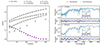 |
Fig. 1. Measure of [α/Fe] on SDSS stacked spectra and associated best-fit spectra. Left panel: Elemental abundances as a function of the velocity dispersion for ETGs. Empty symbols correspond to literature measurements of different α elements. The diamonds indicate average [α/Fe] from Thomas et al. (2010), up and down triangles are oxygen and magnesium as measured by Johansson et al. (2012), and squares show the [Mg/Fe] trend of Conroy et al. (2014). The filled purple circles show the best-fitting (but misleading) pPXF+MILES solution. Right panels: Spectra for the lowest (top panel) and highest (bottom panel) σ bin. The observed stacked spectrum is given in black and the best-fit spectrum in cyan. The residuals are shown in blue. We also provide a zoom-in into the Mgb region. |
To assess the origin of this misleading [α/Fe] trend that results from combining pPXF with the MILES models, we show the best-fit spectra for the lowest and highest σ on the right side of Fig. 1. Even though the residuals are lower than 3%, the magnesium triplet (5175 Å) is clearly not well fit by the models, especially for the high σ bin. This suggests that the [α/Fe] obtained with the MILES models and pPXF do not capture the actual change in [Mg/Fe].
As an additional test, we repeated our stellar population analysis over three different wavelength regions: (1) 4000–4800 Å, (2) 4800–5400 Å and (3) 5400–6600 Å including the Hβ region. We display the results for [α/Fe] in the top panel of Fig. 2 and compare them to our previous results. We obtain similar results, that is, an apparent decrease in [α/Fe] with increasing σ, for the bluest and reddest wavelength regions. Only for the region dominated by the Mgb triplet (green symbols), are we able to recover a flat trend between the measured [α/Fe] and σ.
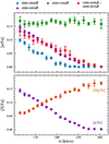 |
Fig. 2. Further measures of [α/Fe], and [Mg/Fe]. Top panel: [α/Fe]–σ relation obtained by fitting the SDSS data over different wavelength ranges: 4000–4800 Å (blue), 4800–5400 Å (green), and 5400–6600 Å including the Hβ region (red). Bottom panel: [X/Fe]–σ relation using magnesium-enhanced models (orange). These models combine the MILES Vazdekis et al. (2015) and the Conroy & Dokkum (2012b) predictions (see details in the text). For reference, the filled purple circles in both panels represent the results from Fig. 1. |
3.2. Individual α-element abundances
The tests above, and in particular, the right panels in Fig. 1, reveal that the combination of α-enhanced MILES models and pPXF cannot model the strength of the Mgb absorption feature properly, which might lead to biased [α/Fe] measurements. We only recover a non-decreasing trend when we focus on the magnesium triplet. Aiming to isolate the effect of [Mg/Fe] on the recovered trends, we repeated our stellar population analysis with a set of magnesium-enhanced models. These models were constructed by combining MILES base models (i.e. with an abundance pattern that traces the [Mg/Fe]–[Fe/H] relation of the solar neighbourhood) with the magnesium response function obtained by Conroy & Dokkum (2012b). After feeding pPXF with these Mg-enhanced models over the entire wavelength range 4000–6600 Å, we obtained the trend shown in the bottom panel of Fig. 2.
The bottom panel of Fig. 2 clearly shows that when fed with Mg-only enhanced models, pPXF is able to recover the expected trend between stellar velocity dispersion and [Mg/Fe] (orange symbols), and it only fails when the input models assume that all α-elements are enhanced (purple symbols). Since in the α-variable MILES models all α-elements are varied in lockstep, it is likely that the trend shown in Fig. 1 is caused by the failure of the different α-elements to track each other as a function of velocity dispersion (e.g., Conroy et al. 2014). We also find similarly spurious trends when using the different predictions of Conroy & Dokkum (2012b) to compute α-variable models, but with fixed relative abundances (e.g. all α-elements are enhanced to the same degree).
To test this hypothesis, we emulated the effect that changes in the mixture of α-elements would have on the observed SDSS data. We constructed SDSS-like mock spectra using the MILES [α/Fe] = 0 models and corrected them with the Conroy & Dokkum (2012b) predictions according to the individual abundance ratios found by Beverage et al. (2023) for C, Mg, Si, Ca, and Ti. This allowed us to explore the effect of measuring [α/Fe] with SSP models that enhance all α-elements simultaneously by the same amount on data for which the elements do not follow this behaviour. Over these mock spectra, we then ran our fiducial stellar population analysis, that is, pPXF plus the α-variable MILES models.
The result of this test is shown in Fig. 3. We recover a remarkably similar decreasing trend of [α/Fe] from the mock spectra (blue symbols) compared to our initial results of the real SDSS data (purple symbols). This suggests that applying models that vary all α-elements by the same amount to data for which different α-elements do not track each other might lead to biased and thus flawed measurements.
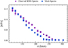 |
Fig. 3. [α/Fe]–σ relation measured from the mock spectra. The blue circles represent the results obtained for the mock spectra that include different abundance patterns for individual α-elements as measured in Beverage et al. 2023; (updated results from Conroy et al. 2014). The filled purple circles again represent the results found in Fig. 1 for comparison purposes. |
Our understanding of this phenomenon relies on the non-uniformity of flux variations caused by the enhancement of individual α-elements. Essentially, an increase in the abundance of individual α-elements can yield deeper absorption features for some elements while weakening them for others (see Conroy et al. 2014, Fig. 2). Therefore, this could result in flux changes that compensate for each other to some extent within specific wavelength regions, even when all these elements are varied by the same amount. This ill-constrained behaviour is further accentuated by the fact that the resulting effective [α/Fe] is weighted by the wavelength-dependent sensitivity to the elemental abundance. Hence, applying a model in which all α-elements are varied in lockstep to a spectrum in which individual α-elements likely have different abundances could result in the FSF trying to fit certain wavelength regions in which the flux change of all the α-elements combined translates into a decreasing [α/Fe] trend. However, it is important to note that all individual α-elements do not truly decrease due to the different relative flux changes described above.
4. Effect of a variable initial mass function on the [Mg/Fe]–σ relation
The results above highlight some of the biases that can occur from an incorrect application of SSP models that enhance all α-elements in the same way, in combination with a large wavelength range, as is the case for a full spectral fitting. This is particularly the case for information that is predominantly concentrated on specific absorption features. In this section, we make use of the high sensitivity of some of these absorption features to revisit the [Mg/Fe]–σ relation in the context of a non-universal IMF.
We followed the full index-fitting (FIF) approach described in Martín-Navarro et al. (2019, 2021) to measure the age, metallicity, [Mg/Fe], IMF slope, and [Ti/Fe] of the stacked SDSS spectra. This fitting approach consists of a Bayesian fit to each pixel within the (continuum-corrected) bandpass definition of a set of key spectral features, which in this case were Hβo, an optimised version of Hβ (Cervantes & Vazdekis 2009), Mgb, Fe 5015, Fe 5270, Fe 5335, TiO1, and TiO2. We used MILES α-enhanced SSP models with a bimodal IMF slope (Vazdekis et al. 1996) ranging from Γb = 0.5 to Γb = 3.5. However, we measured [Mg/Fe] because of the indices we fitted (Martín-Navarro et al. 2019, 2021). In contrast to our previous measurements using pPXF, FIF-based quantities are weighted by luminosity3.
The left panel of Fig. 4 shows our best-fitting [Mg/Fe] values as a function of the stellar velocity dispersion. The measurements allowing for a variable IMF in the fitting process are shown as filled orange symbols, and a fixed Milky Way-like IMF is shown as empty orange symbols. Our measurements based on a universal IMF agree with the literature, as expected. We measure an increase of 0.11 dex in [Mg/Fe] from the lowest to the highest velocity dispersion stacks. A similar trend emerges from the variable IMF results, up to σ ∼ 230 km s−1. However, for σ ≳ 240 km s−1, the trend flattens, resulting in lower [Mg/Fe] for the most massive galaxies. This is ultimately due to the non-negligible dependence of the Mgb absorption feature on the adopted IMF within the MILES models. The IMF slopes retrieved with FIF perfectly agree with the results found in La Barbera et al. (2013). Regardless of the assumptions on the IMF, [Mg/Fe] clearly increases with σ, which emphasises the spurious nature of the trends shown in Fig. 1.
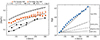 |
Fig. 4. Impact of the IMF on [Mg/Fe] and Mgb measurments. Left panel: [Mg/Fe]–σ relation of our stack spectra using FIF (orange). The empty circles represent the results obtained with a fixed Milky Way-like IMF, and the filled circles show our measurements when the IMF is treated as an additional free parameter. The black lines correspond to literature [Mg/Fe] measurements: Johansson et al. (2012) (solid line), Worthey et al. (2014) (dotted line with data points), Conroy et al. (2014) (dashed line with data points), Thomas et al. (2005) (dash-dotted line), and McDermid et al. (2015) (dashed line). Right panel: Mgb–σ relation of our stack spectra and the relative contribution to the Mgb strength from age, metallicity, [Mg/Fe], and IMF variations. |
To further illustrate the importance of a variable IMF in our interpretation of the [Mg/Fe] enhancements of massive galaxies, the right panel of Fig. 4 shows the age, metallicity, [Mg/Fe], and IMF variations to the empirical Mgb–σ relation. As reported by Thomas et al. (2005), this relation encodes the fact that more massive ETGs are older, more metal rich, and more enhanced in [Mg/Fe] than their low-mass counterparts. However, there is a subtle but noticeable additional contribution to the Mgb strength from the excess of low-mass stars that are contained in the central regions of massive ETGs.
5. Discussion and conclusion
We have demonstrated that the measure of [α/Fe] as a function of σ using pPXF and the MILES SSP models over a wide wavelength range results in an apparently decreasing trend. Even when a narrower wavelength range is selected that focused on the Mgb region, we still did not recover the well-known increasing trend. Moreover, we find significant differences in the recovered trends based on the Vazdekis et al. (2015) or Conroy & Dokkum (2012b) models. Both models lead to spurious results when fed into pPXF, however. These results do not reflect an actual decrease in [α/Fe] for more massive ETGs, but the limitations of FSF algorithms combined with SSP models assuming a fixed mixture of α-elements to capture the complexity of the chemical evolution in galaxies. Discrepancies among the model predictions further emphasise the difficulty of robustly quantifying a single and representative [α/Fe] value.
Our results therefore call for a careful interpretation of [α/Fe] measurements based on the combination of FSF tools and SSP models that only vary the global [α/Fe] value. Since not all α-elements necessarily track each other (e.g. Worthey 1998; Johansson et al. 2012; Conroy et al. 2014; Worthey et al. 2014), the same [α/Fe] can result from several completely different combinations of individual abundances. Furthermore, as revealed by our analysis, [α/Fe] estimates might be completely unphysical when the assumed stellar population models do not allow for relative changes in elemental abundances. This is particularly problematic with FSF algorithms because different α-elements contribute differently and in a highly degenerate manner to absorption spectra of galaxies.
In this context, measurements of individual abundances are more robust quantities, allowing fairer comparisons and a more accurate description of the underlying physical mechanisms controlling the evolution of galaxies. For example, the measure of magnesium is the founding principle of what is now qualified as α-enhancement (Peletier 1989; Worthey et al. 1992). In addition, light α-elements, such as Mg or Si, are more strongly enhanced than heavier α-elements, such as Ca and Ti (Johansson et al. 2012; Conroy et al. 2014; Worthey et al. 2014). Furthermore, Milky Way abundance studies revealed that magnesium is the most robust and consistent α-element (Jönsson et al. 2018; Zasowski et al. 2019). Therefore, [Mg/Fe] alone acts as a better tracer than [α/Fe], as expected.
We also showed that precise [Mg/Fe] are sensitive to IMF variations, in agreement with Conroy et al. (2014). For the most massive galaxies in the SDSS stacked spectra, which exhibit the largest IMF variations, we find [Mg/Fe] values that are lower by ∼0.035 dex than our measurements assuming a Milky Way-like IMF. Under the assumption that [Mg/Fe] scales with the timescales of star formation (e.g. Thomas et al. 2005), our results then indicate that massive ETGs formed their stellar component over relatively longer periods of time than is usually assumed (e.g. McDermid et al. 2015; Segers et al. 2016).
These findings imply that our physical interpretation of the α-enhancement as only reflecting the length of the star formation timescales is not complete and among other aspects, lacks the implications of a varying IMF. A more nuanced interpretation that combines the effect of star formation and the non-universal IMF will be necessary to be better represent the observations. The consideration of a time-varying or a non-canonical IMF will open the door for a more complete and consistent characterisation of the chemical evolution of massive galaxies (e.g. Vazdekis et al. 1997; Ferreras et al. 2015; Jeřábková et al. 2018)
SPectroscopic IDentfication of ERosita Sources.
Given the set of indices included in the analysis of Thomas et al. (2010) it is fair to assume that [α/Fe] in this case corresponds to [Mg/Fe].
pPXF fits a linear combination of multiple SSPs to the observed spectrum, whereas FIF finds the best-fit SSP-equivalent spectrum.
Acknowledgments
We would like to thank the anonymous referee for their detailed comments and suggestions, resulting in an improved version of the manuscript. EP would like to thank Francesco La Barbera for his stacked spectra and insights, and Alexandre Vazdekis for his support and enriching discussions. EP acknowledges support from the Turning Scheme. We acknowledge support from grants PID2019-107427GB-C32 and PID2022-140869NB-I00 from the Spanish Ministry of Science. AB gratefully acknowledges support from the Moritz-Schlick early-career Postdoc Programme.
References
- Adelman-Mccarthy, J. K., Agüeros, M. A., Allam, S. S., et al. 2008, ApJS, 175, 297 [NASA ADS] [CrossRef] [Google Scholar]
- Bacon, R., Conseil, S., Mary, D., et al. 2017, A&A, 608, A1 [NASA ADS] [CrossRef] [EDP Sciences] [Google Scholar]
- Bekki, K. 2013, MNRAS, 436, 2254 [NASA ADS] [CrossRef] [Google Scholar]
- Beverage, A. G., Kriek, M., Conroy, C., et al. 2023, ApJ, 948, 140 [NASA ADS] [CrossRef] [Google Scholar]
- Boecker, A., Leaman, R., van de Ven, G., et al. 2020, MNRAS, 491, 823 [Google Scholar]
- Cappellari, M. 2017, MNRAS, 466, 798 [Google Scholar]
- Cappellari, M., & Emsellem, E. 2004, PASP, 116, 138 [Google Scholar]
- Cappellari, M., McDermid, R. M., Alatalo, K., et al. 2012, Nature, 484, 485 [Google Scholar]
- Cervantes, J. L., & Vazdekis, A. 2009, MNRAS, 392, 691 [NASA ADS] [CrossRef] [Google Scholar]
- Chabrier, G. 2003, PASP, 115, 763 [Google Scholar]
- Conroy, C., & Dokkum, P. G. V. 2012a, ApJ, 760, 71 [NASA ADS] [CrossRef] [Google Scholar]
- Conroy, C., & Dokkum, P. V. 2012b, ApJ, 747, 69 [NASA ADS] [CrossRef] [Google Scholar]
- Conroy, C., Graves, G., & van Dokkum, P. 2014, ApJ, 780, 33 [Google Scholar]
- Faber, S. M., Worthey, G., & Gonzales, J. J. 1992, IAU Symp., 149, 255 [NASA ADS] [Google Scholar]
- Falcón-Barroso, J., Sánchez-Blázquez, P., Vazdekis, A., et al. 2011, A&A, 532, A95 [Google Scholar]
- Ferreras, I., Weidner, C., Vazdekis, A., & La Barbera, F. 2015, MNRAS, 448, L82 [NASA ADS] [CrossRef] [Google Scholar]
- Jeřábková, T., Hasani Zonoozi, A., Kroupa, P., et al. 2018, A&A, 620, A39 [Google Scholar]
- Jönsson, H., Prieto, C. A., Holtzman, J. A., et al. 2018, AJ, 156, 126 [CrossRef] [Google Scholar]
- Johansson, J., Thomas, D., & Maraston, C. 2012, MNRAS, 421, 1908 [NASA ADS] [CrossRef] [Google Scholar]
- Kroupa, P. 2001, MNRAS, 322, 231 [NASA ADS] [CrossRef] [Google Scholar]
- La Barbera, F., Ferreras, I., Vazdekis, A., et al. 2013, MNRAS, 433, 3017 [Google Scholar]
- Martín-Navarro, I., Lyubenova, M., Ven, G. V. D., et al. 2019, A&A, 626, A126 [NASA ADS] [CrossRef] [EDP Sciences] [Google Scholar]
- Martín-Navarro, I., Pinna, F., Coccato, L., et al. 2021, A&A, 654, 59 [Google Scholar]
- Matteucci, F. 1994, A&A, 288, 57 [NASA ADS] [Google Scholar]
- McDermid, R. M., Alatalo, K., Blitz, L., et al. 2015, MNRAS, 448, 3484 [Google Scholar]
- Peletier, R. 1989, Ph.D. Thesis, University of Groningen, The Netherlands [Google Scholar]
- Pietrinferni, A., Cassisi, S., Salaris, M., & Castelli, F. 2004, ApJ, 612, 168 [Google Scholar]
- Pietrinferni, A., Cassisi, S., Salaris, M., & Castelli, F. 2006, ApJ, 642, 797 [Google Scholar]
- Pinna, F., Falcón-Barroso, J., Martig, M., et al. 2019a, A&A, 625, A95 [NASA ADS] [CrossRef] [EDP Sciences] [Google Scholar]
- Pinna, F., Falcón-Barroso, J., Martig, M., et al. 2019b, A&A, 623, A19 [NASA ADS] [CrossRef] [EDP Sciences] [Google Scholar]
- Segers, M. C., Schaye, J., Bower, R. G., et al. 2016, MNRAS, 456, 1235 [NASA ADS] [CrossRef] [Google Scholar]
- Thielemann, F. K., Argast, D., Brachwitz, F., et al. 2003, in From Twilight to Highlight: The Physics of Supernovae, eds. W. Hillebrandt, & B. Leibundgut, (Berlin, Heidelberg: Springer), 331 [Google Scholar]
- Thomas, D., Maraston, C., Bender, R., & Oliveira, C. M. D. 2005, ApJ, 621, 673 [NASA ADS] [CrossRef] [Google Scholar]
- Thomas, D., Maraston, C., Schawinski, K., Sarzi, M., & Silk, J. 2010, MNRAS, 404, 1775 [NASA ADS] [Google Scholar]
- Trager, S. C., Faber, S. M., & Worthey, G. 2000, AJ, 120, 165 [NASA ADS] [CrossRef] [Google Scholar]
- Vazdekis, A., Casuso, E., Peletier, R. F., & Beckman, J. E. 1996, ApJS, 106, 307 [Google Scholar]
- Vazdekis, A., Peletier, R. F., Beckman, J. E., & Casuso, E. 1997, ApJS, 111, 203 [CrossRef] [Google Scholar]
- Vazdekis, A., Sánchez-Blázquez, P., Falcón-Barroso, J., et al. 2010, MNRAS, 404, 1639 [NASA ADS] [Google Scholar]
- Vazdekis, A., Coelho, P., Cassisi, S., et al. 2015, MNRAS, 449, 1177 [Google Scholar]
- Worthey, G. 1998, PASP, 110, 888 [NASA ADS] [CrossRef] [Google Scholar]
- Worthey, G., Faber, S., & Gonzalez, J. 1992, ApJ, 398, 69 [NASA ADS] [CrossRef] [Google Scholar]
- Worthey, G., Tang, B., & Serven, J. 2014, ApJ, 783 [NASA ADS] [CrossRef] [Google Scholar]
- Zasowski, G., Schultheis, M., Hasselquist, S., et al. 2019, ApJ, 870, 138 [NASA ADS] [CrossRef] [Google Scholar]
Appendix A: Variations in the initial mass function of FIF and FSF
We show the [Mg/Fe]–σ using FIF and FSF with both a fixed and variable IMF in Figure A.1.
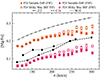 |
Fig. A.1. [Mg/Fe]–σ relation of our stack spectra measured using FSF and Mg-enhanced models (pink) as well as FIF (orange) for a Kroupa universal IMF (empty circles) and a σ-varying IMF (filled circles). The black lines and symbols correspond to works (also shown in Figure 4) that explicitly measured [Mg/Fe]. |
The results obtained with the two methods agree with each other. The difference between the results from FSF and FIF corresponds to a shift of ∼0.1 dex. The same shift is observed between Johansson et al. (2012) and Conroy et al. (2014). These results show that even with FSF, using a wide wavelength range and SSP models that are only enhanced in magnesium, the impact of the IMF can be measured. Moreover, this provides an additional piece of evidence that [Mg/Fe] is a robust α-element.
All Figures
|
Fig. 1. Measure of [α/Fe] on SDSS stacked spectra and associated best-fit spectra. Left panel: Elemental abundances as a function of the velocity dispersion for ETGs. Empty symbols correspond to literature measurements of different α elements. The diamonds indicate average [α/Fe] from Thomas et al. (2010), up and down triangles are oxygen and magnesium as measured by Johansson et al. (2012), and squares show the [Mg/Fe] trend of Conroy et al. (2014). The filled purple circles show the best-fitting (but misleading) pPXF+MILES solution. Right panels: Spectra for the lowest (top panel) and highest (bottom panel) σ bin. The observed stacked spectrum is given in black and the best-fit spectrum in cyan. The residuals are shown in blue. We also provide a zoom-in into the Mgb region. |
| In the text | |
|
Fig. 2. Further measures of [α/Fe], and [Mg/Fe]. Top panel: [α/Fe]–σ relation obtained by fitting the SDSS data over different wavelength ranges: 4000–4800 Å (blue), 4800–5400 Å (green), and 5400–6600 Å including the Hβ region (red). Bottom panel: [X/Fe]–σ relation using magnesium-enhanced models (orange). These models combine the MILES Vazdekis et al. (2015) and the Conroy & Dokkum (2012b) predictions (see details in the text). For reference, the filled purple circles in both panels represent the results from Fig. 1. |
| In the text | |
|
Fig. 3. [α/Fe]–σ relation measured from the mock spectra. The blue circles represent the results obtained for the mock spectra that include different abundance patterns for individual α-elements as measured in Beverage et al. 2023; (updated results from Conroy et al. 2014). The filled purple circles again represent the results found in Fig. 1 for comparison purposes. |
| In the text | |
|
Fig. 4. Impact of the IMF on [Mg/Fe] and Mgb measurments. Left panel: [Mg/Fe]–σ relation of our stack spectra using FIF (orange). The empty circles represent the results obtained with a fixed Milky Way-like IMF, and the filled circles show our measurements when the IMF is treated as an additional free parameter. The black lines correspond to literature [Mg/Fe] measurements: Johansson et al. (2012) (solid line), Worthey et al. (2014) (dotted line with data points), Conroy et al. (2014) (dashed line with data points), Thomas et al. (2005) (dash-dotted line), and McDermid et al. (2015) (dashed line). Right panel: Mgb–σ relation of our stack spectra and the relative contribution to the Mgb strength from age, metallicity, [Mg/Fe], and IMF variations. |
| In the text | |
|
Fig. A.1. [Mg/Fe]–σ relation of our stack spectra measured using FSF and Mg-enhanced models (pink) as well as FIF (orange) for a Kroupa universal IMF (empty circles) and a σ-varying IMF (filled circles). The black lines and symbols correspond to works (also shown in Figure 4) that explicitly measured [Mg/Fe]. |
| In the text | |
Current usage metrics show cumulative count of Article Views (full-text article views including HTML views, PDF and ePub downloads, according to the available data) and Abstracts Views on Vision4Press platform.
Data correspond to usage on the plateform after 2015. The current usage metrics is available 48-96 hours after online publication and is updated daily on week days.
Initial download of the metrics may take a while.