| Issue |
A&A
Volume 682, February 2024
|
|
|---|---|---|
| Article Number | A173 | |
| Number of page(s) | 15 | |
| Section | Interstellar and circumstellar matter | |
| DOI | https://doi.org/10.1051/0004-6361/202348108 | |
| Published online | 23 February 2024 | |
Feedback from protoclusters does not significantly change the kinematic properties of the embedded dense gas structures
1
Max-Planck-Institut für Radioastronomie,
Auf dem Hügel 69,
53121
Bonn,
Germany
e-mail: jwzhou@mpifr-bonn.mpg.de
2
Max Planck Institute for Astronomy,
Königstuhl 17,
69117
Heidelberg,
Germany
3
Shanghai Astronomical Observatory, Chinese Academy of Sciences,
80 Nandan Road,
Shanghai
200030,
PR China
4
Department of Physics; University of Helsinki,
PO Box 64,
00014
Finland
5
Kavli Institute for Astronomy and Astrophysics, Peking University,
Haidian District,
Beijing
100871,
PR China
6
Department of Astronomy, School of Physics, Peking University,
Beijing
100871,
PR China
7
Department of Astronomy, Yunnan University,
Kunming
650091,
PR China
8
Department of Physics, Faculty of Science, Kunming University of Science and Technology,
Kunming
650500,
PR China
9
National Astronomical Observatory of Japan, National Institutes of Natural Sciences,
2-21-1 Osawa,
Mitaka,
Tokyo
181-8588,
Japan
10
Departamento de Astronomía, Universidad de Chile,
Casilla 36-D,
Santiago,
Chile
11
Satyendra Nath Bose National Centre for Basic Sciences,
BlockJD, Sector-III, Salt Lake,
Kolkata-700 106,
India
Received:
28
September
2023
Accepted:
1
December
2023
A total of 64 ATOMS sources at different evolutionary stages were selected to investigate the kinematics and dynamics of gas structures under feedback. We identified dense gas structures based on the integrated intensity map of H13CO+ J = 1−0 emission, and then extracted the average spectra of all the structures to investigate their velocity components and gas kinematics. For the scaling relations between the velocity dispersion, σ, the effective radius, R, and the column density, N, of all the structures, σ − N * R always has a stronger correlation compared to σ − N and σ − R. There are significant correlations between velocity dispersion and column density, which may imply that the velocity dispersion originates in gravitational collapse, also revealed by the velocity gradients. The measured velocity gradients for dense gas structures in early-stage sources and late-stage sources are comparable, indicating gravitational collapse through all evolutionary stages. Late-stage sources do not have large-scale hub-filament structures, but the embedded dense gas structures in late-stage sources show similar kinematic modes to those in early- and middle-stage sources. These results may be explained by the multi-scale hub-filament structures in the clouds. We quantitatively estimated the velocity dispersion generated by the outflows, inflows, ionized gas pressure, and radiation pressure, and found that the ionized gas feedback is stronger than other feedback mechanisms. However, although feedback from HII regions is the strongest, it does not significantly affect the physical properties of the embedded dense gas structures. Combined with the conclusions in our previous work on cloud-clump scales, we suggest that although feedback from cloud to core scales will break up the original cloud complex, the substructures of the original complex can be reorganized into new gravitationally governed configurations around new gravitational centers. This process is accompanied by structural destruction and generation, and changes in gravitational centers, but gravitational collapse is always ongoing.
Key words: techniques: image processing / stars: formation / evolution / ISM: structure / submillimeter: ISM
© The Authors 2024
 Open Access article, published by EDP Sciences, under the terms of the Creative Commons Attribution License (https://creativecommons.org/licenses/by/4.0), which permits unrestricted use, distribution, and reproduction in any medium, provided the original work is properly cited.
This article is published in open access under the Subscribe to Open model.
Open Access funding provided by Max Planck Society.
1 Introduction
Stellar feedback from high-mass stars (M > 8 M⊙) can strongly influence their surrounding interstellar medium and regulate star formation. The combined effects of multiple feedback mechanisms may play a major role in determining star formation efficiency and the initial mass function in molecular clouds (Dib et al. 2010; Krumholz et al. 2014). In Krumholz et al. (2014), feedback mechanisms are divided into three categories: (1) momentum feedback, including protostellar outflows and (probably) radiation pressure; (2) explosive feedback, including winds from hot main sequence stars, photoionizing radiation, and supernovae; and (3) thermal feedback, with non-ionizing radiation as the main form. Lopez et al. (2014) assessed the role of stellar feedback at scales ~10–100 pc toward 32 HII regions in the Large and Small Magellanic Clouds. They employed multi-wavelength data to examine several stellar feedback mechanisms and found that the ionized gas feedback dominates over the other mechanisms in all of the sources. Similar methods were also used in Olivier et al. (2021) but, for 106 deeply embedded HII regions with radii <0.5 pc, they concluded that the dust-processed radiation dominates in 84% of the samples. In simulations, massive stellar feedback, including ionizing radiation, stellar winds, and supernovae (Matzner 2002; Dale et al. 2012, 2014; Rogers & Pittard 2013; Rahner et al. 2017; Smith et al. 2018; Lewis et al. 2023), can suppress star formation and destroy the natal cloud. However, whether stellar feedback promotes or suppresses star formation remains controversial. The simulations of Dale et al. (2014) examined the effects of photoionization and momentum-driven winds from O-stars on molecular clouds, and found that feedback has little effect on denser and more massive clouds, which mainly destroy clouds with a lower density and mass. Dib et al. (2013) showed, using semi-analytical models in which gas-expulsion from protocluster clouds is driven by stellar wind feedback originating from both B and O stars that the gas expulsion timescale depends on the clouds mass and the coupling efficiency of the wind with the surrounding gas. The observations of Pabst et al. (2019), Henshaw et al. (2022) suggest that at early stages energy-winds could dominate, even if this is questioned by recent theoretical works (Lancaster et al. 2021a,b). It is also possible for the feedback to be positive by triggering new star formation. In Deharveng et al. (2005), Zavagno et al. (2006), and Liu et al. (2017), using data at various wavelengths, they identified and studied several objects in which star formation appears to have been triggered at the borders of HII regions. Thompson et al. (2012) studied a large sample of infrared bubbles and estimated that the fraction of massive stars in the Milky Way formed by triggering could be between 14 and 30%. Kendrew et al. (2012) found that approximately ~22% of massive young stars may have formed as a result of feedback from expanding HII regions.
As presented in Watkins et al. (2019), stellar feedback from O stars clearly modifies the structure of the larger-scale clouds, but without much effect on the dynamical properties of the assembled dense gas. In the G305 GMC, feedback has triggered star formation by the collect and collapse mechanism based on observations using the Large APEX sub-Millimeter Array (LAsMA) seven-beam receiver on the 12-meter Atacama Pathfinder Experiment submillimeter telescope (APEX; Mazumdar et al. 2021a,b). In Rugel et al. (2019), feedback from the first formed cluster in W49A is not strong enough to disperse the cloud, which likely only affects limited parts of W49A. Moreover, all feedback models used in Rugel et al. (2019) predict recollapse of the shell after the first star formation event. The importance of large-scale gravitational collapse in star formation regions has been suggested in many observational and theoretical works (Hartmann & Burkert 2007; Vázquez-Semadeni et al. 2009, 2019; Schneider et al. 2010; Peretto et al. 2013, 2014; Wyrowski et al. 2016; Hacar et al. 2017). In a sample of 11 massive clumps, high-resolution data reveal that protoclusters evolves to tighter by global gravitational collapse (Xu et al. 2024). In the LAsMA observation for the G333 complex under feedback, on large scales, (Zhou et al. 2023, 2024) found that the inflow may be driven by the larger-scale structure, consistent with the hierarchical structure in the molecular cloud and gas inflow from large to small scales. The large-scale gas inflow is driven by gravity, implying that the molecular clouds in the G333 complex may be in a state of global gravitational collapse (see also Dib 2023). Ubiquitous density and velocity fluctuations also imply the widespread presence of local gravitational collapse (Henshaw et al. 2020). As for local dense gas structures, most of them exhibit an obvious correlation between velocity dispersion and density, which indicates the gravitational origin of velocity dispersion. For the G333 complex, although the original cloud complex is disrupted by feedback, the substructures of the original complex can be reorganized into new gravitationally governed configurations around new gravitational centers. This process is accompanied by structural destruction and generation and by changes in gravitational centers, but gravitational collapse is always ongoing. The results in (Zhou et al. 2022, 2023, 2024) and Peretto et al. (2023) show that the kinematic properties of parsec-scale clumps in two very different physical environments (infrared dark and infrared bright) are comparable. Thus, feedback in infrared bright star-forming regions, such as the G333 complex, will not change the kinematic properties of parsec-scale clumps, which is also consistent with the survey results that most Galactic parsec-scale massive clumps seem to be gravitationally bound regardless of their evolutionary phases (Liu et al. 2016; Urquhart et al. 2018; Evans et al. 2021).
In this work, we extend the cloud-clump analysis in Zhou et al. (2024) to the clump-core scale using high-resolution ALMA data from the ATOMS (ALMA Three-millimeter Observations of Massive Star-forming regions) survey (Liu et al. 2020). The ATOMS survey has observed 146 active star-forming regions at ALMA Band 3. The data can be used to systematically investigate the spatial distribution of various dense gas tracers in a large sample of Galactic massive clumps. The dense molecular gas structures inside the cloud serve as star-forming sites, their physical states directly determine the star formation capability of the molecular cloud under feedback. A more systematic study is needed to evaluate how massive protostars influence the dense gas distribution and star formation efficiency in their natal clumps. Using ALMA data, we zoomed into the dense gas structures close to or even connecting with protoclusters. The effects of feedback were then inferred through the physical properties of the surrounding dense gas structures. The sample of the ATOMS survey includes 146 active star-forming regions. In Zhou et al. (2022), we find that hub-filament systems are very common within massive protoclusters, and that stellar feedback from HII regions gradually destroys the hub-filament systems as protoclusters evolve. The sources at different evolutionary stages are dominated by different feedback mechanisms. By comparing the physical properties of dense gas structures in the clumps at different evolutionary stages, we will be able to infer the relative importance of various feedback mechanisms.
2 Observations
2.1 ALMA observations
We used ALMA data from the ATOMS survey (Project ID: 2019.1.00685.S; PI: Tie Liu). The ATOMS sources were initially selected from a complete and homogeneous CS J = 2−1 molecular line survey toward IRAS sources with far-infrared colors characteristics of UC HII regions (Bronfman et al. 1996). As discussed in Liu et al. (2020), the ATOMS sources are distributed in very different environments of the Milky Way, and are an unbiased sample of the protoclusters with the strongest CS J = 2−1 line emission (TA > 2 K) located in the inner Galactic plane of −80° < l < 40°, |b| < 2° (Faúndez et al. 2004).
For the data reduction, the details of the 12 m array and 7 m array ALMA observations were summarized in (Liu et al. 2020, 2021). Calibration and imaging were carried out using the CASA software package version 5.6 (McMullin et al. 2007). The 7 m data and 12 m array data were calibrated separately. Then the visibility data from the 7 m and 12 m array configurations were combined and later imaged in CASA. For each source and each spectral window (spw), a line-free frequency range was automatically determined using the ALMA pipeline. This frequency range was used to (a) subtract continuum from line emission in the visibility domain, and (b) make continuum images. Continuum images were made from multifrequency synthesis of data in the line-free frequency ranges in the two 1.875 GHz wide spectral windows, spws 7 and 8, centered on ~99.4 GHz (or 3 mm). Visibility data from the 12 m and 7 m arrays were jointly cleaned using the task tclean in CASA 5.6. We used natural weighting and a multiscale deconvolver for an optimized sensitivity and image quality. All images were primary beam-corrected. The continuum image reaches a typical 1 σ rms noise of ~0.2 mJy with a synthesized beam FWHM size of ~2.2″. In this work, we also used H13CO+ J = 1−0 (86.754288 GHz) and HCO+ J = 1−0 (89.188526 GHz) molecular lines data with spectral resolutions of 0.211 km s−1 and 0.103 km s−1. The typical beam FWHM size and channel rms noise level for H13CO+ J = 1−0 line emission are ~2.5″ and 8 mJy beam−1, respectively. For HCO+ J = 1−0 line emission, the two values are ~2.4″ and 12 mJy beam−1. The typical maximum-recovered angular scale in this survey is about 1 arcmin, which is comparable to the field of view (FOV) in the 12 m array observations (Liu et al. 2020).
2.2 Spitzer infrared data
We also used images at 8.0 µm, obtained by the Spitzer Infrared Array Camera (IRAC), as part of the GLIMPSE project (Benjamin et al. 2003). The images of IRAC were retrieved from the Spitzer Archive and the angular resolution of the images is about 2″.
3 Results
3.1 Evolutionary stages
Generally, the infrared properties and the presence of H40α emission can be used to assess the evolutionary stages of the sources (Chambers et al. 2009; Sanhueza et al. 2012). As discussed in Zhou et al. (2022), stellar feedback from HII regions will gradually destroy the hub-filament systems as protoclusters evolve. Thus, the morphology of the hub-filament structure can also characterize the evolutionary stages. In Figs. 2 and 3 of Zhou et al. (2022), for hub-filament systems, the overlaid contours of the 3 mm continuum should be located at the center of filamentary network with the strongest H13CO+ J = 1−0 emission, where is the center of the gravitational potential well and the potential site for high-mass star formation. In the late stage of evolution, the 3 mm continuum emission is almost completely separated from H13CO+ J = 1−0 emission, indicating that the relatively evolved HII regions have dispersed their natal gas (see also Liu et al. 2023). Thus, the separation between 3 mm continuum emission and H13CO+ (1−0) emission can also be used for the classification. Finally, we divided ATOMS sources into three evolutionary stages using the following criteria:
- 1.
The sources at an early stage (early sources): (1) infrared dark and without H40α emission; (2) well-defined hub-filament structures; and (3) their 3mm continuum emissions concentrate on the centers of filamentary networks with the strongest H13CO+ (1−0) emission.
- 2.
The sources at a middle stage (middle sources) have the same features as the early sources apart from having compact H40α emission.
- 3.
The sources at a late stage (late sources): (1) obvious triggering signs such as the bent dense gas structures traced by H13CO+ (1−0) emission; (2) their 3mm emission is extended, and all of them have strong H40α and 8 µm emission, indicating that 3mm continuum emission is dominated by free-free emission (Keto et al. 2008; Zhang et al. 2023). The two conditions mean that hubs in the late stage have developed into protoclusters. Powerful HII regions driven by protoclusters will destroy the hub-filament systems eventually. We can see the expansion of HII regions is tearing up the surrounding gas structures in Fig. 1c.
The number of early sources, middle sources, and late sources is 30, 11, and 23, respectively. We applied stringent criteria for the selection, and retained only sources that can be clearly categorized in one out of the three stages. The values of the radius, distance, bolometric luminosity, mass, and dust temperature of ATOMS sources are listed in Table A.1 of Liu et al. (2020). The luminosity-to-mass ratios, L/M, and dust temperature, T, of the clumps can be used to trace the evolutionary process of star formation (Saraceno et al. 1996; Krumholz & Tan 2007; Molinari et al. 2008; Liu et al. 2016; Stephens et al. 2016; Urquhart et al. 2018). As shown in Figs. 2c and d, from the early stage through to the middle and late stages, L/M and T of the sources are indeed increasing gradually, confirming that our classification is reasonable.
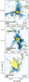 |
Fig. 1 Moment 0 maps of H13CO+ J = 1−0 for three ATOMS sources at three evolutionary stages. Yellow contours show 3 mm continuum emission with its minimum contour level of 5σ. Orange eclipses represent the retained Dendrogram structures. The maps of all 64 ATOMS sources studied in this work are presented in Appendix B. |
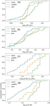 |
Fig. 2 Physical parameters of 64 ATOMS sources at different evolutionary stages. Panels a, b, c, and d show the distributions of the radius. R, distance, D, luminosity-to-mass ratios, L/M, and dust temperature, T, respectively. |
3.2 Dendrogram structures
The issues of identifying the structures in a PPV cube by the dendrogram algorithm are described in Sects. 3.1 and 3.2 of Zhou et al. (2024), and thus we adopted the same method as in Zhou et al. (2024) to identify dense gas structures. We directly identified hierarchical (sub-)structures based on the 2D integrated intensity (moment 0) map of H13CO+ (1−0) emission, and then extracted the average spectrum of each structure to investigate its velocity components and gas kinematics.
For the moment 0 map, a 5σ threshold was set, and we therefore only required the smallest area of the structure to be larger than 0.5 beam and did not set other parameters to reduce the dependence of the identification on the algorithm parameters. In Fig. 1, the structures identified by the dendrogram correspond well to the integrated intensity maps.
The algorithm approximates the morphology of each structure as an ellipse. In the dendrogram, the long and short axes of an ellipse, a and b, are the rms sizes (second moments) of the intensity distribution along the two spatial dimensions. As described in Zhou et al. (2024), a and b will give a smaller ellipse compared to the size of the identified structure, and thus multiplying by a factor of two to enlarge the ellipse is necessary. Then the effective physical radius of an ellipse is  , where D is the distance of the source.
As discussed in Zhou et al. (2024), two screening criteria were used to filter the structures: (1) eliminating the repetitive branch structures; and (2) excluding branch structures with complex morphology. Then for 2477 retained structures, according to their averaged spectra, 57 structures with absorption features were eliminated. Then, following the procedure in Zhou et al. (2024), we fitted the averaged spectra of 2420 structures individually using the fully automated Gaussian decomposer GAUSSPY+ (Lindner et al. 2015; Riener et al. 2019) algorithm. The parameter settings of the decomposition were the same as that in Zhou et al. (2023). According to the line profiles, all the averaged spectra were divided into three categories: type1 (single velocity component, 2038), type2 (separated velocity components, 42), and type3 (blended velocity components, 340). We also refer to Fig. 6 of Zhou et al. (2024) for examples of typical line profiles. In the subsequent analysis, we discarded type2 structures because there are too few of them (1.7%) to simplify the discussion. Furthermore, these structures are likely the product of the overlapping of unrelated gas components.
In this work, we do not classify the structures by the nomenclatures used in astrodendro1, such as leaf, branch, or trunk, because there is always a considerable overlap in the scales between leaf and branch structures, as described in Zhou et al. (2024). Moreover, in Fig. 3, the scales of all structures are presented as a continuous unimodal distribution.
3.3 Column density
To derive the column densities from H13CO+ (1−0) emission, we assumed conditions of local thermodynamic equilibrium (LTE) and a beam filling factor of one. The LTE analysis is described in detail in Appendix A. In Shimajiri et al. (2017), for the Aquila, Ophiuchus, and Orion B clouds, the H13CO+ abundances relative to H2,  , have mean values in the range (1.5−5.8) × 10−11. These abundance estimates are consistent within a factor of a few with the findings in other regions, such as 1.1 ± 0.1×10⁻¹¹ in OMC 2-FIR 4 (Shimajiri et al. 2015) and 1.8 ± 0.4 × 10⁻¹¹ in Sagittarius A (Tsuboi et al. 2011). Peretto et al. (2013) derived a H13CO+ abundance of 5 × 10⁻¹¹ from Mopra observations towards SDC335 using the ID non-LTE RADEX radiative transfer code (van der Tak et al. 2007). Here, we take the mean value
  shown in Table 2 of Shimajiri et al. (2017).
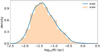 |
Fig. 3 Scale distribution of all identified structures. The probability density was estimated using the kernel density estimation (KDE) method. |
3.4 Velocity components
In Zhou et al. (2024), type3 structures were discarded because of the complex line profiles. In this work, to increase the samples of each source, we needed to consider type3 structures. Possible reasons for the complex profiles were: (1) the optical depth effect; (2) the overlapping of uncorrelated gas components; and (3) the complex gas kinematics inside the structures. Generally, H13CO+ J = 1−0 line emission is optically thin, and thus we did not consider the first factor. The second factor has been discussed in detail in Zhou et al. (2022) and is not an issue in the ATOMS survey, and thus our analysis in the previous work can be done based on the moment maps. The significant overlap for the line profile of a type3 structure may indicate the correlation between different velocity components in the structure. The more severe the overlap between different velocity components, the more likely they belong to the same structure. In the extreme case, they merge into a single-peak line profile. If the velocity differences between different velocity components are small, these velocity components are likely to be different parts of the same structure rather than unrelated overlapping structures, and thus the velocity decomposition is not necessary. For example, in a hub-filament structure, the velocity of gas flow in each filament is different, leading to different velocity components in the same structure. Considering the multi-scale hub-filament scenario described in Zhou et al. (2022), type3 structures may be hub-filament structures at different scales.
In the subsequent analysis, we treat type3 structures as independent structures like type1 structures, but with more complex gas motions. We constantly provide evidence to justify this assumption. If different velocity components in a type3 structure are different parts of the same structure, the velocity dispersion of the type3 structure can be obtained by an intensity-weighted average of the velocity dispersion of all velocity components within this structure.
3.5 Statistics of the basic physical quantities
Below, we discuss the differences in the physical properties of different structure types at different evolutionary stages. For two data sets, the magnitude comparison is based on their median values. Generally, the p value of their Kolmogorov-Smirnov (KS) test is far less than 0.05, if their median values are significantly different, as shown in Fig. 4.
From the first line of Fig. 4, type3 structures have a larger velocity dispersion, higher column density, and lower virial ratios than type1 structures at different evolutionary stages, indicating that type3 structures are mainly concentrated in the hub regions, and thus have a higher column density and present multiple velocity components. In Zhou et al. (2022), from the grid maps of H13CO (1−0) emission, the hub regions always show multiple velocity components that should be attributed to the complex gas motions, not the superposition of uncorrelated foreground or background velocity components.
From the second line of Fig. 4, although late sources have powerful HII regions, their inner gas structures do not have a significantly larger velocity dispersion and virial ratios, compared to that in early and middle sources. In Fig. 4e, the embedded dense structures inside middle sources even have a slightly larger velocity dispersion than those inside late sources. These statistical results are unusual. We need to reconsider the effects of feedback from expanding HII regions (see Sect. 3.8 for more discussion.) Moreover, the higher column density of the embedded dense structures inside middle sources in Fig. 4f is in line with the gravitational collapse of hub-filament systems.
3.6 Scaling relations
The scaling relations between different quantities contain information on the physical conditions of the structures. The scaling relations between the velocity dispersion, σ, effective radius, R, and column density, N, shown in Fig. 5 are similar to those in Zhou et al. (2024). σ − N * R always has a stronger correlation compared to σ − N and σ − R2. However, the slopes of σ − N * R relations are ~0.27, which may indicate the slowing down of a pure free-fall gravitational collapse. There are significant correlations between velocity dispersion and column density, which may imply that the velocity dispersion originates from the gravitational collapse, something which is also revealed by the measured velocity gradients in Sect. 3.7. σ − R has a poor correlation, that is, a significant deviation from the Larson-relation (Larson 1981).
Additionally, it is noteworthy that both type 1 and type3 structures present similar scaling relations, which further confirms that type3 structures are independent like type1 structures. The structures generated by random overlap should not show good scaling relations.
3.7 Velocity gradient
In Zhou et al. (2022), we used the moment 0 maps (integrated intensity maps) of H13CO+ J = 1−0 to identify filaments in ATOMS sources, and extracted the velocity and intensity along the filament skeletons from the moment 1 and moment 0 maps. Clear velocity and density fluctuations are seen along the filaments, allowing us to fit velocity gradients around the intensity peaks. The filaments like the streamlines, which can trace how gas inflows converge to local dense structures. Local dense structures as gravitational centers will accrete the surrounding diffuse gases and then form local hub-filament structures. A hub-filament structure can be translated into a funnel structure in the PPV space, as described in Zhou et al. (2023). As illustrated in Fig. 9 of Zhou et al. (2023), the gradient of the funnel profile can reflect the strength of the gravitational field. In Zhou et al. (2022, 2023), the filaments will pass through multiple local hub-filament structures presented as velocity and density fluctuations. Therefore, the local velocity gradients along the filaments can reveal the strength of local gravitational fields. Then, by comparing local velocity gradients, we can assess the differences in the gravitational states of the embedded dense gas structures among different feedback environments.
For all ATOMS sources, the identified filaments, and corresponding extracted velocity and density along the filaments, have been shown in Zhou et al. (2022). We first estimated two overall velocity gradients between the velocity peaks and valleys at the two sides of the center of the gravitational potential well and ignored the local velocity fluctuation, then we also derived local velocity gradients around local intensity peaks of the H13CO+ emission (see Fig. 6 in Zhou et al. 2022). In Fig. 4g, the virial ratios of the embedded dense gas structures in late and early sources are comparable. In Fig. 6, the measured velocity gradients of the structures in early and late sources are also comparable, once again demonstrating that feedback rarely affects the physical properties of the embedded dense gas structures.
 |
Fig. 4 Physical properties of different structure types at different evolutionary stages. The first row is the comparison between type1 and type3 structures. The second row is the comparison between early, middle and late sources. The dashed lines in panels c and g mark the positions of αvir = 2. “p” is the p value of the Kolmogorov–Smirnov (KS) test. “p12,” “pl3,” and “p23” are the p values of KS tests between the structures inside early and middle sources, early and late sources, and middle and late sources, respectively. The median values also show in the legends. |
3.8 Feedback of early sources versus late ones
In an analysis of the kinematics in early sources, we mainly focused on the outflows and inflows. When investigating the gas kinematics in late sources, we primarily considered the ionized gas pressure. Moreover, the radiation pressure exists in all sources at different evolutionary stages. But late sources must have stronger radiation pressure than early sources, because they embed luminous ionizing (young) stellar objects. We note that inflow is not a feedback mechanism; but as a line-broadening mechanism, it is comparable to other feedback mechanisms. Below, we quantitatively estimate the velocity dispersion generated by the four physical processes, and then compare them with the statistical results in Sect. 3.5.
3.8.1 Outflow
We assumed that the line emission of H13CO+ J = 1−0 and high velocity emission of HCO+ J = 1−0 are optically thin, and that the excitation temperatures of the H13CO+ J = 1−0 and HCO+ J = 1−0 lines are the same and constant in both low-and high-velocity outflow gas. Then, according to Eqs. (4) and (5) in Zhou et al. (2021), the mass of the outflows can be estimated by
![${{{M_{{\rm{out}}}}} \over {{M_{{\rm{gas}}}}}} \approx \left[ {{{{{\rm{H}}^{13}}{\rm{C}}{{\rm{O}}^ + }} \over {{\rm{HC}}{{\rm{O}}^ + }}}} \right]{{{F_{{\rm{out}},{\rm{HC}}{{\rm{O}}^ + }}}} \over {{F_{{\rm{gas}},{{\rm{H}}^{13}}{\rm{C}}{{\rm{O}}^ + }}}}}.$](/articles/aa/full_html/2024/02/aa48108-23/aa48108-23-eq4.png) (1)
(1)
The expression in brackets is the abundance ratio of the molecules. Here, we took [H13CO+/HCO+] ~ 1/60 (Milam et al. 2005).  and
and  are the corresponding total velocity-integrated fluxes (the sum of all pixels in the moment 0 maps) of the outflows and dense gases of the clump traced by the HCO+ (1−0) and H13CO+ (1−0) emission. Mgas was calculated using the column density map derived by LTE analysis in Sect. 3.6. After obtaining the value of Mout, according to the total velocity-integrated flux of the redshifted and blueshifted lobes of the outflows
  and
and  , the masses of the two lobes were
 (2)
(2)

Assuming that the momentum of the outflows completely transfers to the surrounding dense gas (i.e., the upper limit), then the corresponding turbulent velocity, υturb,out, inside the dense gas caused by the outflows can be estimated from the equation
 (4)
(4)
According to the moment 1 maps of the two lobes, their average velocities are υr0 and υb0, the systematic velocity of the clump is υ0, and then the velocities of the two lobes are υr = υr0 − υ0 and υb = υ0 − υb0.
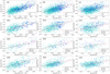 |
Fig. 5 Scaling relations of type1 and type3 structures, (a) σ − N * R, (b) σ − N, and (c) σ − R. σ, R and N are the velocity dispersion, effective radius, and column density of each structure, respectively, “r” represents the Pearson correlation coefficient. The values in the legends are the exponents of the power laws. The second, third, and fourth rows are the same as the first row, but for early, middle and late sources, respectively. |
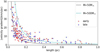 |
Fig. 6 Velocity gradient versus the length over which the gradient has been fitted. Blue and red crosses represent the velocity gradients fitted in early and late sources, respectively. The dashed lines show free-fall velocity gradients for comparison. For the free-fall model, black and cyan lines denote masses of 50 M⊙ and 500 M⊙, respectively. |
3.8.2 Inflow
Assuming spherical symmetry, the clump has a mass inflow rate of
 (5)
(5)

Rc and Mc are the radius and mass of the clump, respectively, rin and υin are the infall radius and velocity. We note that the distance, D, radius, Rc, dust temperature, Td, mass, Mc, and bolometric luminosity, Lbol, of the clumps were taken as the values listed in Table A.1 of Liu et al. (2020). For clumps to be hub-filament systems, they should be in a state of global gravitational collapse, and thus we assumed that Rc = rin.
For the inflow rate,  , of the clump, the tables in He et al. (2015, 2016) listed mass infall rates of 231 clumps. Based on the tables, we fitted the quantitative relation between the inflow rate and the mass of the clump, as shown in Fig. 7. Then the infall rates of early sources could be estimated using this relation according to their masses. Finally, the infall velocity could be estimated by
 (7)
(7)
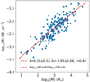 |
Fig. 7 The relation between the inflow rate and the mass of the clump. Data points are from the tables of He et al. (2015, 2016). “r” is the Pearson coefficient. |
3.8.3 Radiation pressure
Following Lopez et al. (2014), the volume-averaged radiation pressure, Prad, is
 (8)
(8)
Lbol is the bolometric luminosity of the clump.
3.8.4 Ionized gas pressure
Following Lopez et al. (2014), the ionized gas pressure is given by the ideal gas law, PHII = (ne + nH + nHe)kTHII, where ne, nH, and nHe are the electron, hydrogen, and helium number densities, respectively, and THII is the temperature of the HII gas, which was assumed to be the same for electrons and ions. If helium is singly ionized, then ne + nH + nHe ≈ 2ne. The electron temperature and density of resolved UC HII regions identified in the ATOMS survey were derived from radio recombination lines, H40α, and 3 mm continuum emission in Zhang et al. (2023). The corresponding velocities contributed by Prad and PHII were estimated by  .
.
3.8.5 Relative importance of feedback processes
In Tables 1 and 2, υHII is significantly larger than other velocities, consistent with the conclusions in Lopez et al. (2014) that the ionized gas feedback dominates over the other considered feedback mechanisms. In this work, we did not intend to study which feedback mechanism is the strongest, and thus we ignored some feedback mechanisms, such as dust-reprocessed radiation and stellar wind, which may also play important roles (Pabst et al. 2019; Olivier et al. 2021; Henshaw et al. 2022). Here, we note that the estimated υHII is obviously larger than the observed line widths in H13CO+ J = 1−0. This is not surprising because the energy is deposited into the ionized gas and photodisso-ciation regions. As expected, late sources present significantly stronger radiation pressure than early sources. For early sources, the velocity dispersion caused by the outflows is significantly smaller than that from the infalls and the radiation pressure.
Velocity dispersion produced by different physical processes in early sources.
4 Discussion
4.1 Gravitational collapse under feedback
As discussed in Sect. 3.7, even under strong feedback, the embedded dense structures in late sources can still retain gravitational collapse. Feedback may redistribute local dense gas structures, as illustrated in Fig. 8, because feedback does not seem to affect the internal dynamics of the embedded dense gas structures. The results are consistent with the conclusion in Zhou et al. (2024): although the feedback disrupting the molecular clouds will break up the original cloud complex, the substructures of the original complex can be reorganized into new gravitationally governed configurations around new gravitational centers. This process is accompanied by structural destruction and generation, and by changes in gravitational centers, but gravitational collapse is always ongoing.
Moreover, in Fig. 6, we can find the same gas kinematic mode presented in Zhou et al. (2023). The variations in the velocity gradients at small and large scales (~0.2 pc as the boundary) are consistent with gravitational free-fall, with central masses of ~50 M⊙ and ~500 M⊙. It means that the velocity gradients on larger scales require larger masses to be maintained, and larger masses imply larger scales; that is to say, the larger-scale inflow is driven by the larger-scale structure, which may be the gravitational clustering of smaller-scale structures, consistent with the hierarchical or multi-scale hub-filament structures in the clouds and the gas inflow from large to small scales. In Zhou et al. (2023), we studied the gas motions of the G333 molecular cloud complex. The longest filament is ~50 pc; however, the largest scale in Fig. 6 is only ~1 pc. The similar gas kinematic modes may indicate the self-similar kinematic structures on cloud-clump and clump-core scales, as illustrated in Fig. 9 of Zhou et al. (2023).
Velocity dispersion produced by different physical processes in late sources.
4.2 The role of feedback
In Sect. 3.8, the significantly larger υHII will naturally make us think that late sources should have the strongest feedback effects. However, that is not the case, as shown in Sect. 3.5. In Sect. 3.5, overall, the velocity dispersion and virial ratios of the structures inside early and late sources are comparable. As shown in Sect. 3.7, the gas structures in late sources are also in gravitational collapse like those in early sources. Gravitational collapse may also contribute significantly to the velocity dispersion of the gas structures in late sources. Thus, the proportion of the velocity dispersion of the gas structures contributed by expanding HII regions in late sources decreases further. The clouds exist as gas reservoirs that contain dense gas structures as local gravitational centers. Feedback from HII regions destroys the clouds by mechanical force; in other words, the expanding HII regions push away and reshape the loose cloud complex (see e.g., McLeod et al. 2015; Beuther et al. 2022; Bonne et al. 2023). But the processes do not significantly affect the physical properties of the embedded dense gas structures in the clouds, suggesting that HII regions may not effectively inject momentum into the embedded dense gas structures as star-forming sites. However, the triggering does not necessarily result from momentum being transferred inside the gas structures but by the gas structures being compressed, and so becoming gravitationally unstable.
Although the feedback from HII regions is very strong, it is acting from the outside on the embedded dense gas structures. By comparison, the outflows and inflows can go deep inside of the embedded dense gas structures, and thus the effect of them on the physical properties of the gas structures is not necessarily weaker than the feedback from HII regions. We should not only focus on the strength of a feedback mechanism itself, but also assess the extent to which it can affect the embedded dense gas structures.
In Fig. 4e, the structures in middle sources display a slightly larger velocity dispersion than those in late sources. Notably, middle-stage sources possess larger-scale hub-filament structures than their late-stage counterparts. The complex gas kinematics in these hub regions within middle-stage sources may contribute to the higher velocity dispersion observed. Furthermore, early sources also exhibit large-scale hub-filament structures, but their gas structures present a smaller velocity dispersion compared to those in middle sources. This suggests that feedback from UC-HII regions in middle sources plays a significant role. At least, we can conclude that feedback from protocluster-driven HII regions may not be the most powerful factor affecting the physical properties of local dense gas structures. It is important to note that the above discussion treats each clump in isolation, without considering the potential effects of the surrounding gas environment on the physical properties of the internal structures of the clumps, due to the limited FOV of ALMA observations. Given that the protocluster-driven HII regions may still be bound by the abundant surrounding gas, possible quasi-static expanding processes also indicate the limited effect of feedback from HII regions on the embedded dense gas structures. As shown in Kuhn et al. (2019), star clusters and associations that are still embedded in molecular clouds are less likely to be expanding than those that are partially or fully revealed.
As illustrated in Fig. 8, hierarchical hub-filament structures of star-forming regions mean that star-forming regions exist as loose gravitational complexes. Feedback will reshape the overall structures of star-forming regions. This process is accompanied by the redistribution of the internal structures of the clouds, while the gravitational coupling between the internal structures also reorganizes them into new gravitationally governed configurations around new gravitational centers. Generally, feedback will disperse the clouds. Finally, to some extent, the reorganization is a resistance to the dispersing process, although the resistance will in the end fail. The negative effects of the feedback are that it destroys the gas reservoir inhabited by dense gas structures, inhibiting the further growth of dense structures by accreting the surrounding gas, and thus suppressing the formation of massive stars. On the other hand, if feedback makes the dense gas structures more spread out, and if these dense structures are still in a gas-rich environment, the looser distribution will improve the material accumulation efficiency of the dense structures by weakening the competitive accretion between them, and may eventually form more massive stars.
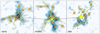 |
Fig. 8 Schematic diagram of the scenario argued in this work. Evolution of a cloud with multi-scale hub-filament structures with increasing effects of feedback. Here we borrowed three pictures from Fig. 1 as the background, for demonstration only. The yellow lines are the filament skeletons identified in Zhou et al. (2022). Considering the competitive accretion scenario, the precursor of the protocluster is located in the central position of the hub. With the evolution of the protocluster, feedback from HII regions destroys the hub by mechanical force, i.e., the expanding HII regions push away and reshape the hub region, accompanied by the redistribution of small-scale dense structures that may be local hub-filament structures. We note that small-scale hub-filament structures were not directly identified in this work due to the limitation of the resolution. |
5 Summary
A total of 64 ATOMS sources at different evolutionary stages were selected to investigate the kinematics and dynamics of gas structures under feedback.
- 1.
We directly identified dense gas structures based on the 2D integrated intensity (moment 0) map of H13CO+ (1–0) emission, and then extracted the average spectrum of each structure to investigate their velocity components and gas kinematics. We discussed the differences in the physical properties of different structure types at different evolutionary stages. (1) Type3 structures with blended velocity components (see Fig. 6 of Zhou et al. 2024) have a larger velocity dispersion, higher column density, and lower virial ratios than type1 structures with a single velocity component at different evolutionary stages, which can be attributed to type3 structures being mainly located in hub regions. (2) Overall, the velocity dispersion and virial ratios of the structures inside early and late sources are comparable. The structures inside middle sources even have a slightly larger velocity dispersion than those inside late sources. These unusual results led us to question the effectiveness of feedback from HII regions in late sources.
- 2.
σ − N * R always has a stronger correlation than σ − N and σ − R. There are significant correlations between velocity dispersion and column density, which may imply that the velocity dispersion originates in the gravitational collapse, something also revealed by the measured velocity gradients. Type1 and type3 structures present similar scaling relations, which further confirms that type3 structures are independent structures, not the superposition of uncorrelated foreground or background velocity components.
- 3.
Dense gas structures in late sources are in gravitational collapse like those in early sources. Late sources do not have large-scale hub-filament structures, but the embedded dense gas structures in late sources show similar kinematic modes to those in early and middle sources. These results may be explained by the multi-scale hub-filament structures in the clouds.
- 4.
The differences in the gravitational states of dense gas structures in different feedback environments were investigated by comparing local velocity gradients. The measured velocity gradients of the structures in early and late sources are comparable, indicating that feedback has a limited impact on the kinematic properties of local dense gas structures. The velocity gradients on larger scales require a larger mass to be maintained, and larger masses imply larger scales; that is to say, the larger-scale inflow is driven by the larger-scale structure, which may be the gravitational clustering of smaller-scale structures, consistent with the hierarchical or multi-scale hub-filament structures in the clouds and the gas inflow from large to small scales.
- 5.
We quantitatively estimated the velocity dispersion generated by the outflows, inflows, ionized gas pressure, and radiation pressure, and found that the ionized gas feedback is stronger than other feedback mechanisms. Late sources present significantly stronger radiation pressure than early sources. For early sources, the velocity dispersion caused by the outflows is significantly smaller than that from the infalls and the radiation pressure. However, although feedback from HII regions is the strongest, it does not significantly affect the physical properties of the embedded dense gas structures in the clumps, suggesting that HII regions may not effectively inject momentum into the embedded dense gas structures as star-forming sites.
- 6.
This work on clump-core scales reaches the same conclusion as the study of the G333 molecular cloud complex on cloud-clump scales in Zhou et al. (2024), and thus we suggest that although feedback from cloud to core scales will break up the original cloud complex, the substructures of the original complex can be reorganized into a new gravitationally governed configuration around new gravitational centers. This process is accompanied by structural destruction and generation, and by changes in gravitational centers, but gravitational collapse is always ongoing.
Acknowledgements
We would like to thank the referee for the detailed and constructive comments and suggestions that significantly improve and clarify this work. We thank J.H. He to share the tables of their studied infall samples. This paper makes use of the following ALMA data: ADS/JAO.ALMA#2019.1.00685.S. ALMA is a partnership of ESO (representing its member states), NSF (USA) and NINS (Japan), together with NRC (Canada), MOST and ASIAA (Taiwan), and KASI (Republic of Korea), in cooperation with the Republic of Chile. The Joint ALMA Observatory is operated by ESO, AUI/NRAO and NAOJ.
Appendix A LTE analysis
Following the procedures described in Garden et al. (1991); Mangum & Shirley (2015), for a rotational transition from the upper level, J + 1, to the lower level, J, we can derive the total column density by
![${N_{tot{\rm{ }}}} = {{3k} \over {8{\pi ^3}{\mu ^2}B(J + 1)}}{{\left. {\left( {{T_{{\rm{ex}}}} + hB/3k} \right)\exp \left[ {hBJ(J + 1)/k{T_{{\rm{ex}}}}} \right)} \right]} \over {1 - \exp \left( { - hv/k{T_{{\rm{ex}}}}} \right)}}\int \tau {\rm{dv}},$](/articles/aa/full_html/2024/02/aa48108-23/aa48108-23-eq18.png) (A.1)
(A.1)
![$\tau = - \ln \left[ {1 - {{{T_{{\rm{mb}}}}} \over {J\left( {{T_{{\rm{ex}}}}} \right) - J\left( {{T_{{\rm{bg}}}}} \right)}}} \right],$](/articles/aa/full_html/2024/02/aa48108-23/aa48108-23-eq19.png) (A.2)
(A.2)
 (A.3)
(A.3)
 (A.4)
(A.4)
where B = v/[2(J + 1)] is the rotational constant of the molecule, μ is the permanent dipole moment, and μ = 3.89 Debye for H13CO+. Tbg = 2.73 K is the background temperature and ∫ Tmbdv represents the integrated intensity. In the above formulas, the correction for high optical depth was applied (Frerking et al. 1982; Goldsmith et al. 2008; Areal et al. 2019). Assuming optically thick emission of HCO+ (1–0) emission, we can estimate the excitation temperature, Tex, following the formula (Garden et al. 1991; Pineda et al. 2008)
![${T_{{\rm{ex}}}} = {{4.28} \over {\ln \left[ {1 + 1/\left( {0.23{T_{{\rm{peak }}}} + 0.26} \right)} \right]}},$](/articles/aa/full_html/2024/02/aa48108-23/aa48108-23-eq22.png) (A.5)
(A.5)
where Tpeak is the observed HCO+ (1–0) peak brightness temperature.
Appendix B The maps of all samples
References
- Areal, M. B., Paron, S., Ortega, M. E., & Duvidovich, L. 2019, PASA, 36, e049 [NASA ADS] [CrossRef] [Google Scholar]
- Ballesteros-Paredes, J., Hartmann, L. W., Vázquez-Semadeni, E., Heitsch, F., & Zamora-Avilés, M. A. 2011, MNRAS, 411, 65 [NASA ADS] [CrossRef] [Google Scholar]
- Benjamin, R. A., Churchwell, E., Babler, B. L., et al. 2003, PASP, 115, 953 [Google Scholar]
- Beuther, H., Schneider, N., Simon, R., et al. 2022, A&A, 659, A77 [NASA ADS] [CrossRef] [EDP Sciences] [Google Scholar]
- Bonne, L., Kabanovic, S., Schneider, N., et al. 2023, A&A, 679, L5 [NASA ADS] [CrossRef] [EDP Sciences] [Google Scholar]
- Bronfman, L., Nyman, L. A., & May, J. 1996, A&AS, 115, 81 [Google Scholar]
- Chambers, E. T., Jackson, J. M., Rathborne, J. M., & Simon, R. 2009, ApJS, 181, 360 [NASA ADS] [CrossRef] [Google Scholar]
- Dale, J. E., Ercolano, B., & Bonnell, I. A. 2012, MNRAS, 424, 377 [NASA ADS] [CrossRef] [Google Scholar]
- Dale, J. E., Ngoumou, J., Ercolano, B., & Bonnell, I. A. 2014, MNRAS, 442, 694 [Google Scholar]
- Deharveng, L., Zavagno, A., & Caplan, J. 2005, A&A, 433, 565 [NASA ADS] [CrossRef] [EDP Sciences] [Google Scholar]
- Dib, S. 2023, MNRAS, 524, 1625 [NASA ADS] [CrossRef] [Google Scholar]
- Dib, S., Shadmehri, M., Padoan, P., et al. 2010, MNRAS, 405, 401 [NASA ADS] [Google Scholar]
- Dib, S., Gutkin, J., Brandner, W., & Basu, S. 2013, MNRAS, 436, 3727 [NASA ADS] [CrossRef] [Google Scholar]
- Evans, N. J. II, Heyer, M., Miville-Deschênes, M.-A., Nguyen-Luong, Q., & Merello, M. 2021, ApJ, 920, 126 [NASA ADS] [CrossRef] [Google Scholar]
- Faúndez, S., Bronfman, L., Garay, G., et al. 2004, A&A, 426, 97 [Google Scholar]
- Frerking, M. A., Langer, W. D., & Wilson, R. W. 1982, ApJ, 262, 590 [Google Scholar]
- Garden, R. P., Hayashi, M., Gatley, I., Hasegawa, T., & Kaifu, N. 1991, ApJ, 374, 540 [NASA ADS] [CrossRef] [Google Scholar]
- Goldsmith, P. F., Heyer, M., Narayanan, G., et al. 2008, ApJ, 680, 428 [Google Scholar]
- Hacar, A., Alves, J., Tafalla, M., & Goicoechea, J. R. 2017, A&A, 602, L2 [NASA ADS] [CrossRef] [EDP Sciences] [Google Scholar]
- Hartmann, L., & Burkert, A. 2007, ApJ, 654, 988 [NASA ADS] [CrossRef] [Google Scholar]
- He, Y.-X., Zhou, J.-J., Esimbek, J., et al. 2015, MNRAS, 450, 1926 [NASA ADS] [CrossRef] [Google Scholar]
- He, Y.-X., Zhou, J.-J., Esimbek, J., et al. 2016, MNRAS, 461, 2288 [NASA ADS] [CrossRef] [Google Scholar]
- Henshaw, J. D., Kruijssen, J. M. D., Longmore, S. N., et al. 2020, Nat. Astron., 4, 1064 [CrossRef] [Google Scholar]
- Henshaw, J. D., Krumholz, M. R., Butterfield, N. O., et al. 2022, MNRAS, 509, 4758 [Google Scholar]
- Kendrew, S., Simpson, R., Bressert, E., et al. 2012, ApJ, 755, 71 [NASA ADS] [CrossRef] [Google Scholar]
- Keto, E., Zhang, Q., & Kurtz, S. 2008, ApJ, 672, 423 [NASA ADS] [CrossRef] [Google Scholar]
- Krumholz, M. R., & Tan, J. C. 2007, ApJ, 654, 304 [NASA ADS] [CrossRef] [Google Scholar]
- Krumholz, M. R., Bate, M. R., Arce, H. G., et al. 2014, in Protostars and Planets VI, eds. H. Beuther, R. S. Klessen, C. P. Dullemond, & T. Henning, 243 [Google Scholar]
- Kuhn, M. A., Hillenbrand, L. A., Sills, A., Feigelson, E. D., & Getman, K. V. 2019, ApJ, 870, 32 [CrossRef] [Google Scholar]
- Lancaster, L., Ostriker, E. C., Kim, J.-G., & Kim, C.-G. 2021a, ApJ, 914, 90 [NASA ADS] [CrossRef] [Google Scholar]
- Lancaster, L., Ostriker, E. C., Kim, J.-G., & Kim, C.-G. 2021b, ApJ, 922, L3 [NASA ADS] [CrossRef] [Google Scholar]
- Larson, R. B. 1981, MNRAS, 194, 809 [Google Scholar]
- Lewis, S. C., McMillan, S. L. W., Low, M.-M. M., et al. 2023, ApJ, 944, 211 [NASA ADS] [CrossRef] [Google Scholar]
- Lindner, R. R., Vera-Ciro, C., Murray, C. E., et al. 2015, AJ, 149, 138 [NASA ADS] [CrossRef] [Google Scholar]
- Liu, T., Kim, K.-T., Yoo, H., et al. 2016, ApJ, 829, 59 [NASA ADS] [CrossRef] [Google Scholar]
- Liu, H.-L., Figueira, M., Zavagno, A., et al. 2017, A&A, 602, A95 [NASA ADS] [CrossRef] [EDP Sciences] [Google Scholar]
- Liu, T., Evans, N. J., Kim, K.-T., et al. 2020, MNRAS, 496, 2790 [Google Scholar]
- Liu, H.-L., Liu, T., Evans, Neal J., I., et al. 2021, MNRAS, 505, 2801 [NASA ADS] [CrossRef] [Google Scholar]
- Liu, H.-L., Tej, A., Liu, T., et al. 2023, MNRAS, 522, 3719 [NASA ADS] [CrossRef] [Google Scholar]
- Lopez, L. A., Krumholz, M. R., Bolatto, A. D., et al. 2014, ApJ, 795, 121 [NASA ADS] [CrossRef] [Google Scholar]
- Mangum, J. G., & Shirley, Y. L. 2015, PASP, 127, 266 [Google Scholar]
- Matzner, C. D. 2002, ApJ, 566, 302 [NASA ADS] [CrossRef] [Google Scholar]
- Mazumdar, P., Wyrowski, F., Colombo, D., et al. 2021a, A&A, 650, A164 [NASA ADS] [CrossRef] [EDP Sciences] [Google Scholar]
- Mazumdar, P., Wyrowski, F., Urquhart, J. S., et al. 2021b, A&A, 656, A101 [NASA ADS] [CrossRef] [EDP Sciences] [Google Scholar]
- McLeod, A. F., Dale, J. E., Ginsburg, A., et al. 2015, MNRAS, 450, 1057 [NASA ADS] [CrossRef] [Google Scholar]
- McMullin, J. P., Waters, B., Schiebel, D., Young, W., & Golap, K. 2007, in Astronomical Data Analysis Software and Systems XVI, eds. R. A. Shaw, F. Hill, & D. J. Bell, Astronomical Society of the Pacific Conference Series 376, 127 [NASA ADS] [Google Scholar]
- Milam, S. N., Savage, C., Brewster, M. A., Ziurys, L. M., & Wyckoff, S. 2005, ApJ, 634, 1126 [Google Scholar]
- Molinari, S., Pezzuto, S., Cesaroni, R., et al. 2008, A&A, 481, 345 [NASA ADS] [CrossRef] [EDP Sciences] [Google Scholar]
- Olivier, G. M., Lopez, L. A., Rosen, A. L., et al. 2021, ApJ, 908, 68 [NASA ADS] [CrossRef] [Google Scholar]
- Pabst, C., Higgins, R., Goicoechea, J. R., et al. 2019, Nature, 565, 618 [NASA ADS] [CrossRef] [Google Scholar]
- Peretto, N., Fuller, G. A., Duarte-Cabral, A., et al. 2013, A&A, 555, A112 [NASA ADS] [CrossRef] [EDP Sciences] [Google Scholar]
- Peretto, N., Fuller, G. A., André, P., et al. 2014, A&A, 561, A83 [NASA ADS] [CrossRef] [EDP Sciences] [Google Scholar]
- Peretto, N., Rigby, A. J., Louvet, F., et al. 2023, MNRAS, 525, 2935 [NASA ADS] [CrossRef] [Google Scholar]
- Pineda, J. E., Caselli, P., & Goodman, A. A. 2008, ApJ, 679, 481 [Google Scholar]
- Rahner, D., Pellegrini, E. W., Glover, S. C. O., & Klessen, R. S. 2017, MNRAS, 470, 4453 [NASA ADS] [CrossRef] [Google Scholar]
- Riener, M., Kainulainen, J., Henshaw, J. D., et al. 2019, A&A, 628, A78 [NASA ADS] [CrossRef] [EDP Sciences] [Google Scholar]
- Rogers, H., & Pittard, J. M. 2013, MNRAS, 431, 1337 [CrossRef] [Google Scholar]
- Rugel, M. R., Rahner, D., Beuther, H., et al. 2019, A&A, 622, A48 [NASA ADS] [CrossRef] [EDP Sciences] [Google Scholar]
- Sanhueza, P., Jackson, J. M., Foster, J. B., et al. 2012, ApJ, 756, 60 [Google Scholar]
- Saraceno, P., Andre, P., Ceccarelli, C., Griffin, M., & Molinari, S. 1996, A&A, 309, 827 [Google Scholar]
- Schneider, N., Csengeri, T., Bontemps, S., et al. 2010, A&A, 520, A49 [CrossRef] [EDP Sciences] [Google Scholar]
- Shimajiri, Y., Kitamura, Y., Nakamura, F., et al. 2015, ApJS, 217, 7 [NASA ADS] [CrossRef] [Google Scholar]
- Shimajiri, Y., André, P., Braine, J., et al. 2017, A&A, 604, A74 [NASA ADS] [CrossRef] [EDP Sciences] [Google Scholar]
- Smith, M. C., Sijacki, D., & Shen, S. 2018, MNRAS, 478, 302 [NASA ADS] [CrossRef] [Google Scholar]
- Stephens, I. W., Jackson, J. M., Whitaker, J. S., et al. 2016, ApJ, 824, 29 [NASA ADS] [CrossRef] [Google Scholar]
- Thompson, M. A., Urquhart, J. S., Moore, T. J. T., & Morgan, L. K. 2012, MNRAS, 421, 408 [NASA ADS] [Google Scholar]
- Tsuboi, M., Tadaki, K.-I., Miyazaki, A., & Handa, T. 2011, PASJ, 63, 763 [NASA ADS] [CrossRef] [Google Scholar]
- Urquhart, J. S., König, C., Giannetti, A., et al. 2018, MNRAS, 473, 1059 [Google Scholar]
- van der Tak, F. F. S., Black, J. H., Schöier, F. L., Jansen, D. J., & van Dishoeck, E. F. 2007, A&A, 468, 627 [NASA ADS] [CrossRef] [EDP Sciences] [Google Scholar]
- Vázquez-Semadeni, E., Gómez, G. C., Jappsen, A. K., Ballesteros-Paredes, J., & Klessen, R. S. 2009, ApJ, 707, 1023 [CrossRef] [Google Scholar]
- Vázquez-Semadeni, E., Palau, A., Ballesteros-Paredes, J., Gómez, G. C., & Zamora-Avilés, M. 2019, MNRAS, 490, 3061 [Google Scholar]
- Watkins, E. J., Peretto, N., Marsh, K., & Fuller, G. A. 2019, A&A, 628, A21 [NASA ADS] [CrossRef] [EDP Sciences] [Google Scholar]
- Wyrowski, F., Güsten, R., Menten, K. M., et al. 2016, A&A, 585, A149 [NASA ADS] [CrossRef] [EDP Sciences] [Google Scholar]
- Xu, F., Wang, K., Liu, T., et al. 2024, ApJS, 270, 9 [NASA ADS] [CrossRef] [Google Scholar]
- Zavagno, A., Deharveng, L., Comerón, F., et al. 2006, A&A, 446, 171 [NASA ADS] [CrossRef] [EDP Sciences] [Google Scholar]
- Zhang, C., Zhu, F.-Y., Liu, T., et al. 2023, MNRAS, 520, 3245 [NASA ADS] [CrossRef] [Google Scholar]
- Zhou, J.-W., Liu, T., Li, J.-Z., et al. 2021, MNRAS, 508, 4639 [NASA ADS] [CrossRef] [Google Scholar]
- Zhou, J.-W., Liu, T., Evans, N. J., et al. 2022, MNRAS, 514, 6038 [NASA ADS] [CrossRef] [Google Scholar]
- Zhou, J. W., Wyrowski, F., Neupane, S., et al. 2023, A&A, 676, A69 [NASA ADS] [CrossRef] [EDP Sciences] [Google Scholar]
- Zhou, J. W., Wyrowski, F., Neupane, S., et al. 2024, A&A, 682, A128 [NASA ADS] [CrossRef] [EDP Sciences] [Google Scholar]
For a more convenient comparison with the σ−R and σ−N relations, we converted the Heyer relation, σ/R0.5 ∝ N0.5, to the form σ ∝ (R * N)0.5 (Eq.(3) in Ballesteros-Paredes et al. 2011). Both should have a slope of 0.5.
All Tables
All Figures
|
Fig. 1 Moment 0 maps of H13CO+ J = 1−0 for three ATOMS sources at three evolutionary stages. Yellow contours show 3 mm continuum emission with its minimum contour level of 5σ. Orange eclipses represent the retained Dendrogram structures. The maps of all 64 ATOMS sources studied in this work are presented in Appendix B. |
| In the text | |
|
Fig. 2 Physical parameters of 64 ATOMS sources at different evolutionary stages. Panels a, b, c, and d show the distributions of the radius. R, distance, D, luminosity-to-mass ratios, L/M, and dust temperature, T, respectively. |
| In the text | |
|
Fig. 3 Scale distribution of all identified structures. The probability density was estimated using the kernel density estimation (KDE) method. |
| In the text | |
|
Fig. 4 Physical properties of different structure types at different evolutionary stages. The first row is the comparison between type1 and type3 structures. The second row is the comparison between early, middle and late sources. The dashed lines in panels c and g mark the positions of αvir = 2. “p” is the p value of the Kolmogorov–Smirnov (KS) test. “p12,” “pl3,” and “p23” are the p values of KS tests between the structures inside early and middle sources, early and late sources, and middle and late sources, respectively. The median values also show in the legends. |
| In the text | |
|
Fig. 5 Scaling relations of type1 and type3 structures, (a) σ − N * R, (b) σ − N, and (c) σ − R. σ, R and N are the velocity dispersion, effective radius, and column density of each structure, respectively, “r” represents the Pearson correlation coefficient. The values in the legends are the exponents of the power laws. The second, third, and fourth rows are the same as the first row, but for early, middle and late sources, respectively. |
| In the text | |
|
Fig. 6 Velocity gradient versus the length over which the gradient has been fitted. Blue and red crosses represent the velocity gradients fitted in early and late sources, respectively. The dashed lines show free-fall velocity gradients for comparison. For the free-fall model, black and cyan lines denote masses of 50 M⊙ and 500 M⊙, respectively. |
| In the text | |
|
Fig. 7 The relation between the inflow rate and the mass of the clump. Data points are from the tables of He et al. (2015, 2016). “r” is the Pearson coefficient. |
| In the text | |
|
Fig. 8 Schematic diagram of the scenario argued in this work. Evolution of a cloud with multi-scale hub-filament structures with increasing effects of feedback. Here we borrowed three pictures from Fig. 1 as the background, for demonstration only. The yellow lines are the filament skeletons identified in Zhou et al. (2022). Considering the competitive accretion scenario, the precursor of the protocluster is located in the central position of the hub. With the evolution of the protocluster, feedback from HII regions destroys the hub by mechanical force, i.e., the expanding HII regions push away and reshape the hub region, accompanied by the redistribution of small-scale dense structures that may be local hub-filament structures. We note that small-scale hub-filament structures were not directly identified in this work due to the limitation of the resolution. |
| In the text | |
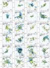 |
Fig. B.1 Same as Fig. 1. |
| In the text | |
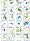 |
Fig. B.2 Same as Fig. 1. |
| In the text | |
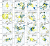 |
Fig. B.3 Same as Fig. 1. |
| In the text | |
Current usage metrics show cumulative count of Article Views (full-text article views including HTML views, PDF and ePub downloads, according to the available data) and Abstracts Views on Vision4Press platform.
Data correspond to usage on the plateform after 2015. The current usage metrics is available 48-96 hours after online publication and is updated daily on week days.
Initial download of the metrics may take a while.