| Issue |
A&A
Volume 685, May 2024
|
|
|---|---|---|
| Article Number | A39 | |
| Number of page(s) | 11 | |
| Section | Interstellar and circumstellar matter | |
| DOI | https://doi.org/10.1051/0004-6361/202347952 | |
| Published online | 03 May 2024 | |
New method for estimating molecular cloud distances based on Gaia, 2MASS, and the TRILEGAL galaxy model
1
Center for Astronomy and Space Sciences, China Three Gorges University,
8 University Road,
443002
Yichang,
PR China
2
College of Science, China Three Gorges University,
8 University Road,
443002
Yichang,
PR China
3
Purple Mountain Observatory, Chinese Academy of Sciences,
10 Yuanhua Road,
210023
Nanjing,
PR China
e-mail: This email address is being protected from spambots. You need JavaScript enabled to view it.
4
University of Science and Technology of China, Chinese Academy of Sciences,
Hefei
230026,
PR China
Received:
12
September
2023
Accepted:
13
February
2024
Abstract
We propose a new method for estimating the distances of molecular clouds traced by CO line emission. Stars from 2MASS and Gaia EDR3 are selected as on-cloud stars when they are projected on a cloud. The background on-cloud stars have redder colors on average than the foreground stars. Instead of searching for stars projected away from the cloud, we employed the TRILEGA galaxy model to mimic the stellar population without cloud extinction along the sightline toward the cloud. Our method does not require an exact boundary of a cloud. The boundaries are highly variable and depend on the sensitivity of the molecular line data. For each cloud, we compared the distributions of on-cloud stars to the TRILEGAL stellar populations in the diagram of J−Ks color versus distance. The intrinsic J−Ks colors of main-sequence and evolved stars from TRILEGAL were considered separately, and they were used as the baseline for subtracting the observed J−Ks colors. The baseline-corrected J−Ks color was deployed with the Bayesian analysis and Markov chain Monte Carlo sampling to determine the distance at which the J−Ks color jump is largest. This method was successfully applied to measure the distances of 27 molecular clouds, which were selected from previously published cloud samples. By replacing TRILEGAL with the GALAXIA galaxy model, we were able to measure the distances for 21 of the 27 clouds. The distances of the 21 clouds based on the GALAXIA model agree well with those based on the TRILEGAL model. The distances of the 27 clouds estimated by this method are consistent with previous estimates. We will apply this new method to a larger region of the gaseous galactic plane, in particular, for the inner galactic region, where a region free of CO emission is hard to separate from the crowded field of clouds.
Key words: stars: distances / ISM: clouds / dust, extinction
© The Authors 2024
 Open Access article, published by EDP Sciences, under the terms of the Creative Commons Attribution License (https://creativecommons.org/licenses/by/4.0), which permits unrestricted use, distribution, and reproduction in any medium, provided the original work is properly cited.
This article is published in open access under the Subscribe to Open model. This email address is being protected from spambots. You need JavaScript enabled to view it. to support open access publication.
1 Introduction
Molecular clouds are the birthplaces of stars. The distance is an important parameter of a molecular cloud when the intrinsic physical properties (mass and size) are to be estimated. Determining the distances of molecular clouds is crucial for characterizing the initial conditions of star formation (McKee & Ostriker 2007; Kennicutt & Evans 2012; Heyer & Dame 2015) and the gaseous spiral arms of the Milky Way (Dame et al. 2001; Xu et al. 2018).
It is always a challenging task to determine the distances of molecular clouds. Several methods were applied to estimate the distances of molecular clouds. The distances of molecular clouds can be estimated from their radial velocities (Vlsr), which are assumed to be attributed to the large-scale rotation of the spiral arms of the Milky Way. The distances estimated from Vlsr of molecular clouds are commonly referred to as kinematic distances (Roman-Duval et al. 2009; Reid et al. 2014). The kinematic distances have large uncertainties and ambiguity problems, especially in the inner Galaxy. The cloud distances can also be estimated by identifying objects associated with or within the molecular cloud, such as OB-associations, young open clusters, H II regions, young stellar objects (YSOs), and masers, whose distances are measured from the trigonometric parallaxes or photometry of stars (Xu et al. 2006; Russeil et al. 2007; Reid et al. 2019; Castro-Ginard et al. 2021; Marton et al. 2023; Zhang 2023). The trigonometric parallaxes measured by Gaia (Gaia Collaboration 2016) for stars up to several kiloparsec provide another approach for estimating the distances of molecular clouds by locating the extinction break point along the line of sight (LOS) toward molecular clouds.
The extinction method relies on accurately estimating the distance and extinction of numerous stars. Green et al. (2014) presented a method for deriving reddening and distances of stars from Panoramic Survey Telescope and Rapid Response System (PanSTARRS-1) photometry and produced a three-dimensional (3D) dust map. Based on the technique of Green et al. (2014), Schlafly et al. (2014) simultaneously inferred the reddening and distances of stars. They measured the distances of molecular clouds selected from the catalog of Magnani et al. (1985) by their extinction break point. The release of astrometric data from Gaia has brought about significant changes in measuring the distance, as it provides a more precise stellar parallax. Combined with Gaia data, several studies presented new 3D extinction maps and have estimated the extinction and distances for millions of stars (Green et al. 2019; Chen et al. 2019; Lallement et al. 2019; Guo et al. 2021; Sun et al. 2021a). One approach involves modeling the dust extinction profiles along different LOS, where the measured cloud is searched for dust clouds from 3D dust structures (Chen et al. 2020b; Guo et al. 2022). Another approach involves searching for the location of the extinction break point that is caused by molecular clouds (Yan et al. 2019; Zucker et al. 2019, 2020; Chen et al. 2020a; Sun et al. 2021b). It can also be applied to supernova remnants (Shan et al. 2019; Wang et al. 2020; Zhao et al. 2020; Leike et al. 2021).
In this work, we make a new attempt to estimate the molecular cloud distances. Principally, stars in front of a molecular cloud have bluer colors on average than those behind a cloud. Instead of searching for stars around the molecular cloud (off-cloud stars), we use the TRILEGAL galaxy model (Girardi 2016) to mimic the stellar population without cloud extinction along the LOS toward the cloud. This means that our method does not depend strongly on the exact boundary of a cloud. The TRILEGAL model is able to simulate stellar populations along sightlines. We fit the baseline separately for main-sequence (MSs) and red giant stars (RGs) to calibrate the corresponding stellar colors. We have estimated the distances of measured molecular clouds from Yan et al. (2021) to confirm the reliability of the method.
The paper is structured as follows. In Sect. 2, we describe the data. In Sect. 3, we introduce our method for estimating the distances of molecular clouds. We present our results and discussions in Sect. 4. We summarize in Sect. 5.
2 Data
Although the bulk masses of molecular clouds are contributed by molecular hydrogen, molecular clouds are well traced by the 12CO molecule, which is the most abundant molecule in molecular clouds after molecular hydrogen. The J = 1−0 transition line emission of 12CO can be observed from ground-based radio telescopes through the atmospheric window at the 3 millimeter wavelength (Dame et al. 2001). In contrast to the 13CO and C18O J = 1−0 emission, 12CO J = 1−0 emission is extended and strong, and it is therefore often chosen to construct the inventory of molecular clouds. We used the 12CO J = 1−0 line emission data from the Milky Way Imaging Scroll Painting (MWISP1) survey by the Purple Mountain Observatory (PMO) 13.7 m millimeter telescope, located at Delingha in China (see more details of MWISP in Su et al. 2019). The rms noise of the 12CO emission of the MWISP survey is about 0.5 K at a velocity resolution of 0.16 km−1 and a grid spacing of 30" × 30". The half-power beamwidth (HPBW) of the 13.7 m telescope at 115 GHz is 50".
Molecular clouds are identified from the 12CO J = 1−0 emission using the DBSCAN algorithm (Ester et al. 1996). Yan et al. (2021) applied DBSCAN to identify molecular clouds from the MWISP 12CO J = 1−0 line emission between l = 25º–50º and in the velocity range −6 to 30 km s−1. By setting the two DBSCAN parameters Eps=1 and MinPts=4, they extracted 359 molecular clouds and measured distances for 27 molecular clouds using the background-eliminated extinction-parallax II (BEEP-II) method. For simplicity, we chose 27 molecular clouds with distance estimates from the cloud sample in Yan et al. (2021) and used the cloud G045.1-03.4 as an example to explain our method, which we present in this work.
We used the astrometric catalog Gaia Early Release 3 (Gaia EDR3; Gaia Collaboration 2021) and the near-IR photometry catalog Two Micron All Sky Survey (2MASS; Skrutskie et al. 2006). The Gaia EDR3 consists of astrometry and photometry for 1.8 billion sources, which improves the parallax precision by 30% over that of Gaia Data Release 2 (Gaia DR2; Gaia Collaboration 2018). The adopted stellar distances were estimated by Bailer-Jones et al. (2021), who transferred the Gaia EDR3 parallaxes to distances using a Bayesian approach. The 2MASS was conducted with two 1.3 m telescopes to provide full sky coverage. It has three near-IR bands, J, H, and Ks, centered at 1.25, 1.65, and 2.16 µm, respectively. The systematic uncertainties of 2MASS photometric measurements are <0.03 mag.
We merged the Gaia and 2MASS catalogs using a cross-match radius of 1" and took the J−Ks color from the 2MASS catalog (Cutri et al. 2003) and the distance from Bailer-Jones et al. (2021). The uncertainty of the stellar distance, Δd, is defined as
 (1)
(1)
where dupper and dlower are the 16th and 84th percentiles of the distance given by Bailer-Jones et al. (2021). The uncertainty of the J−Ks color, Δ(J−Ks), was propagated from the photometric uncertainties in the J and Ks bands.
3 Method
The light passing through a molecular cloud is attenuated by dust within the cloud. The average color of the background stars behind a molecular cloud is redder than that of the foreground stars. The basic idea is to compare the colors of background stars to those of foreground stars, and to locate the distance at which the color difference due to cloud extinction is most prominent. This distance is regarded as the distance to the molecular cloud. This approach greatly benefits from the precise trigonometric parallaxes of billions of stars measured by Gaia.
3.1 Selection of on-cloud stars
For each of the 27 clouds in this work, we searched for stars from the merged Gaia-2MASS catalog based on the position and size of the cloud. A large number of stars can be found within a certain radius for each cloud. We selected the stars projected on the cloud, called on-cloud stars. There are three criteria for selecting the on-cloud stars: (1) The stars lie within the irregular boundary of the molecular cloud. (2) The relative uncertainty of the stellar distance is lower than 10%, that is, Δd/d ≤ 0.1. (3) For each cloud, we calculated a mean rms noise, σint, of integrated CO emission (WCO), based on the 12CO spectra of a cloud in a certain velocity range. We set a threshold COcut = 5σint. On-cloud stars falling within areas with WCO ≥ COcut were kept. The above criteria can be adjusted to optimize the sample size of selected on-cloud stars for each of the 27 clouds. We can increase the COcut to enhance the contrast of J−Ks colors between foreground and background stars. When the selected on-cloud stars for a cloud were not sufficient, we decreased the COcut to gather more on-cloud stars. As an example shown in the left panel of Fig. 1, the selected on-cloud stars (cyan points) for the G045.1-03.4 cloud are overlaid on the integrated-intensity map of the 12CO emission for the cloud. The right panel of Fig. 1 presents the diagram of the J−Ks color versus stellar distance of the selected on-cloud stars for the G045.1-03.4 cloud. In the color-distance diagram, stellar colors start to split into two trends at distance ≳1 kpc. We examine the two trends below, in combination with synthetic stellar population.
3.2 Synthesized stellar population by the TRILEGAL galaxy model
The distributions of on-cloud stars in the color-distance diagram were compared with the synthetic stellar population, which was adopted from the TRILEGAL galaxy model (Girardi 2016). Chen et al. (2022) compared the J−Ks colors of stars toward RCW 120 to the synthetic stellar population of the TRILEGAL galaxy model. Stars with distances ≲1.5 kpc match the TRILE-GAL stellar population in the color-distance diagram well (c.f. Fig.3 in Chen et al. 2022). For each cloud, we generated a collection of synthetic stellar populations within an area slightly larger than the cloud from the online input form of TRILEGAL 1.62. We tweaked the options provided in the online input form of TRILEGAL 1.6. We chose the binary-corrected initial mass function (IMF) of single stars with a break point at 0.5 M⊙ (Kroupa 2002). The photometry system was set to 2MASS JHKs. For each cloud, we adjusted the limiting magnitude in the Ks band by directly counting the Ks-band magnitudes of the on-cloud stars. The distance modulus resolution of the Galaxy components is 0.05 mag. The online input form of TRILEGAL 1.6 provides the option for the dust extinction attributed to the diffuse interstellar medium (ISM) along the sight line. We selected several areas free of 12CO J = 1−0 line emission to simulate the diffuse ISM, and adjusted the Ks-band limiting magnitudes for these areas. We find a good match in the color-distance diagram between the 2MASS+Gaia combination toward these cloud-free areas and the TRILEGAL stellar population with the dust extinction trend of Av/d = 1 mag kpc−1. The 1σ dispersion of the extinction is 0.01 times the total extinction. The Sun is located at a galactocentric distance of 8700 pc and at a height of 24.2 pc along the galactic disk. For the thin disk, we chose a squared hyperbolic secant along z, sech2(0.5z/hz,d), where hz,d increases with age t (hz,d = z0(1 + t/t0)α). The thick disk, similar to the thin disk, is described by a sech2 function, sech2(0.5z/hz,td). The halo is represented by an oblate spheroid with a r1/4 density profile, and the bulge is modeled as a triaxial structure. The output parameters of TRILEGAL mainly include the Galactic component (selecting the thin disk is sufficient), age, luminosity, effective temperature, surface gravity (log g), absolute distance modulus, apparent magnitude in desired filters, and mass.
The TRILEGAL stellar population generated with the above tweaks populate the color-distance diagram similarly to the 2MASS+Gaia combination, as shown in the left panel of Fig. 2, for instance. As a comparison, the right panel of Fig. 2 presents the same stellar populations in the Gaia GBP − GRP versus distance diagram. The TRILEGAL stellar population generally reproduces the observations in both J−Ks and GBP − GRP colors. However, TRILEGAL predicts stellar colors that are more compatible with the 2MASs photometric data than with the Gaia photometric data. The GBP − GRP colors of TRILEGAL are lower than the observed values by Gaia for late-type dwarf stars, which are at closer distances with intrinsically red colors. The TRILEGAL model adopts RV = 3.1 as the default extinction law. The GBP − GRP colors are more sensitive to dust extinction than the J−Ks colors. Any differential from the nominal RV = 3.1 extinction law might lead to an observable mismatch between the observed and synthetic GBP − GRP colors. A detailed comparison between TRILEGAL model and various photometric surveys is beyond the scope of this work. For simplicity, we use the 2MASS+Gaia combination in the following analysis.
Figure 3 compares the TRILEGAL stellar population with the 2MASS+Gaia combination in the Ks versus J−Ks diagram for G045.1-03.4. The Ks-band limiting magnitude was set to 14 mag for TRILEGAL to generate the synthesized stellar population. Fewer than 10% of the observed stars have a Ks magnitude fainter than 14 mag, corresponding to the few stars lying above the truncation of the Ks magnitude for the synthesized stellar population. These faint stars are at distances closer than about 1.5 kpc and are intrinsically red with J−Ks > 0.6, suggesting that they are cool dwarf stars. For most of the observed stars, the synthesized stellar population matches the observations in the Ks versus J−Ks diagram well. The synthesized and observed populations both present two dominant branches that split at J−Ks ≈ 0.7–0.8. We argue that the TRILEGAL galaxy model can be used to generate a synthesized stellar population along the LOS toward molecular clouds, but without cloud extinction. We computed a TRILEGAL stellar population for each of the 27 molecular clouds. Instead of searching off-cloud stars, we used the J−Ks color and distance of each synthesized star to simulate the baseline attributed to the diffuse ISM in the color–distance diagram.
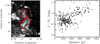 |
Fig. 1 Left panel: selected on-cloud stars for G045.1-03.4. The red contour shows the molecular cloud footprint, and the cyan points represent on-cloud stars. Right panel: J−Ks color vs. distance diagram. It has two branches. |
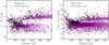 |
Fig. 2 Left and right panels: J−Ks color vs. distance and GBP − GRP color vs. distance diagram for G045.1-03.4, respectively. The purple squares represent the model data, and the black points represent the observation data. |
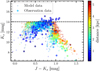 |
Fig. 3 Ks vs. J−Ks diagram of the observation and model data for G045.1-03.4. The squares represent the model data, the hollow circles represent the observation data, and the color represents the distance. The dashed black line is Ks = 14 mag. |
3.3 Elimination of background
The observed and synthesized stellar populations both start to split into two branches at a distance of ≳ 1 kpc in the color–distance diagram, as shown in Fig. 4. The synthesized stellar population at a distance of ≳1 kpc with J–Ks > 0.8 is dominated by RGs with log g < 3.45, while MSs are generally of bluer colors J−Ks < 0.8 at the same distances. By adopting the log g estimates from Gaia DR3 (Gaia Collaboration 2023; Andrae et al. 2023), the observed stars with Gaia DR3 log g estimates are displayed with different colors in Fig. 4. The log g distributions of the observed stars match the TRILEGAL predictions well. MSs of higher log g are distinct from RGs of lower log g in the color–distance diagram. Cool MSs with 0.7 < J − Ks < 1.1 are usually faint sources that are only visible at distances < 1 kpc. As the distance increases, cool MSs become very faint and escape detection by 2MASS, but MSs of earlier types remain detectable. This distance dilution effect is seen for the observed and synthesized populations, that is, the J−Ks colors of MSs become bluer with increasing distance (see also Chen et al. 2022).
We classified the TRILEGAL stellar population into MSs and RGs based on the modeled log g of each simulated star. For simplicity, MSs were defined to have log g > 3.45, and RGs have log g < 3.45. The MSs and RGs samples of TRILEGAL were separately as depicted in the left and right panels of Fig. 5, respectively. We chose a bin of 50 pc to obtain the median colors of MSs and RGs in each distance bin. This is shown as the green and orange squares in the left and right panels of Fig. 5, respectively. We further applied a polynomial fit to the median colors of MSs and a linear fit to the median colors of RGs at various distances, and we obtained the two color baselines shown in Fig. 5: the MSs and the RGs baselines.
Different from the TRILEGAL model without cloud extinction, the observed stars that are located behind molecular clouds are reddened due to cloud extinction along the LOS. Cloud extinction leads to higher J−Ks colors for MSs, resulting in the degeneracy between reddened MSs and RGs on colors. Although Gaia DR3 estimated log g for numerous stars from their low-resolution spectra in the Gaia GBP and GRP bands, the low-resolution spectra of reddened MSs are likely analogous to those of the RGs. The degeneracy between reddened MSs and RGs still remains. The stars at a distance>1 kpc of with J−Ks > 0.8 might originally be RGs or MSs that are reddened by a certain amount of cloud extinction. For example, late-F MSs with intrinsic colors of J−Ks ≈ 0.3 are still detectable by 2MASS and Gaia, even when they are reddened to J−Ks ~ 0.8− 1.0 by cloud extinction of Av ~ 2.5–3.5. The 27 clouds studied in this work are generally not dense; otherwise, we expect very few background stars with a Gaia detection.
The stars with distances greater than 1 kpc and colors exceeding the 3σ lower bound line of RGs baseline are more likely to be RGs, which are marked as red dots in the left panel of Fig. 6. Considering the degeneracy between reddened MSs and RGs on colors, we binned every 100 pc for the observed and synthesized populations simultaneously, and we sorted the observed colors for each distance bin. We further distinguished reddened MSs and RGs according to the fractions of MSs and RGs in TRILEGAL, as illustrated in the right panel of Fig. 6. We subtracted the corresponding model-fit baseline from (reddened) MSs and RGs of the observation data. Figure 7 displays the distribution of baseline-subtracted data. The blue points (binned every 50 pc) are only used for inspection by eyes and not to estimate the distance.
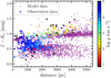 |
Fig. 4 Distributions of the observation and model data in the color-distance diagram for G045.1-03.4. The purple squares represent the model data, the colored points represent the observation data with log g, and the black points represent the observation data without log g. |
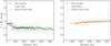 |
Fig. 5 Left and right panels: fit baselines for MSs (dashed black line) and for RGs (dashed red line) in the model data, respectively. The gray squares present the model data. The green and orange squares present the binned MSs and RGs stars (every 50 pc), respectively. |
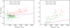 |
Fig. 6 Left panel: distinguished MSs and RGs in the observation data using the 3σ lower bound line of the model-fit RGs baseline (dashed purple line) and a distance of 1 kpc. Right panel: further distinction between the RGs and reddened stars for the differentiated RGs, and reddened stars are classified as MSs. The green and red points show the MSs and RGs of the observation data, respectively. |
3.4 Bayesian analysis and Markov chain Monte Carlo sampling
We adopted a Bayesian analysis and Markov chain Monte Carlo (MCMC) sampling to derive the molecular cloud distances from the baseline-subtracted data. After subtracting the baseline, the color distribution of on-cloud stars became regular and approximately Gaussian. The stellar reddening caused by the molecular cloud remained. In order to estimate the molecular cloud distance, the Bayesian model used in Yan et al. (2019) was adopted. We assumed that the distribution of diffuse dust in the on-cloud region is approximately uniform and that a star is either in front of or behind a molecular cloud. Given a molecular cloud distance (D), the probability that the star is a foreground star is
 (2)
(2)
where  is the cumulative distribution function (CDF) of a Gaussian function, and di and Δdi are the on-cloud star distance and its standard deviation, respectively. Then, the probability that the star is a background star is (1 − fi). The probability density function (PDF) of the Gaussian distribution with a mean µ and a standard deviation σ is
 (3)
(3)
The likelihoods of the foreground and background stars are denoted as
 (4)
(4)
 (5)
(5)
Therefore, the likelihood of a star is
 (6)
(6)
The total likelihood is the product of N on-cloud star likelihoods, that is,
 (7)
(7)
The Bayesian model contains five parameters: the molecular cloud distance (D), the mean (µ1) and standard deviation (σ1) of the foreground star colors, and the mean (µ2) and standard deviation (σ2) of the background star colors. For each molecular cloud, we assumed that the prior distribution of five parameters (D, µ1, σ1, µ2, and σ2) was a uniform distribution, denoting the minimum and maximum of the on-cloud stars as Dmin and Dmax. To prevent the MCMC process from considering all stars as background stars for convergence to small molecular cloud distances, we adjusted the distance minimum to be located 200 pc after the nearest star distance, that is, D ~ U[Dmin + 200, Dmax], where U represents a uniform distribution. Moreover, we required that the mean value µ1 of the foreground star colors must be lower than the mean value µ2 of the background star colors and that the standard deviations (σ1 and σ2) of the foreground and background stars were greater than 0, that is,
 (8)
(8)
We used the MCMC algorithm (Foreman-Mackey et al. 2013) EMCEE package to derive the parameters and uncertainties. For each parameter, we adopted 10 000 steps with 10 walkers to run. The last 1000 steps from each walker were used to sample the final posterior. The results for each parameter approximate a Gaussian distribution. We took the 50th percentile value of the posterior distribution as the best estimate of the parameter, with the uncertainties derived from the 16th and 84th percentile values. To avoid the influence of farther molecular clouds, we set a maximum distance (Dcut) for each molecular cloud. This value was set before estimating clouds distances, which is equivalent to a recursive process. We determined it by eye from the baseline-subtracted data and adjusted it by the near or far distance of the measured molecular cloud. As demonstrated in Fig. 8, we display the estimated distance for G045.1-03.4 based on the MCMC sampling. The corner plots show the five parameters D, µ1, σ1, µ2, and σ2, together with their 50th, 16th, and 84th percentile. The distance of the G045.1-03.4 molecular cloud is  .
.
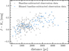 |
Fig. 7 Distribution of the observation data after the color is calibrated. The gray points present the baseline-subtracted observation data. The blue points plot the mean color of the binned stars (every 50 pc for the distance), which are only used to confirm the results for inspection by eye and not to calculate the distance. |
4 Result and discussion
4.1 Distances of the molecular clouds
With the above new method, we derived the distances of 27 molecular clouds. The results are summarized in Table 1. The systematic error is not included. From left to right, we display the molecular cloud name (1), the ratio of the distance errors to the distance (2), the minimum CO emission of the on-cloud stars (3), the maximum distances to the on-cloud stars (4), the number of the on-cloud stars (5), the estimated distances based on the TRILEGAL model (6), the estimated distances based on the GALAXIA model (7), and the distances of Yan et al. (2021) (8). The nearest distance to these molecular clouds is 315 pc, and the farthest distance is 2730 pc. The distance uncertainties might be larger for distant molecular clouds, such as G032.9-01.8 and G042.9+04.4. The results for G045.1-03.4 and G043.3+03.1 are displayed in Figs. 8 and 9, and the other 25 molecular clouds are illustrated in the online supplementary material3.
4.2 Effect of the parameter choice
We explored the effect of the method dependence parameters. In the selection of the on-cloud stars, we involved the COcut parameter above which on-cloud stars are selected. The choice of COcut may affect the determination of the distance. We examined the COcut parameter. To explore the influence of this parameter, we only changed the COcut and left other parameters unchanged, and we compared the molecular cloud distance variations. As shown in Fig. 10, we display the molecular cloud distances and uncertainties after changing COcut, and the range of COcut is taken as 3σint ~ 7σint. The distance uncertainty of G042.9+04.4 is larger than that of G045.4-04.2 because the fewer background stars of the far-distant molecular cloud result in a larger distance uncertainty. There are slight fluctuations in the molecular cloud distances and uncertainties, but they are within reasonable limits. In general, COcut has only a weak effect on the distance estimate. Thus, the new method does not depend strongly on the boundary of the cloud.
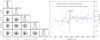 |
Fig. 8 Distances of GO45.1-03.4. The corner plots of the MCMC samples of five modeled parameters and their uncertainties are displayed on the left. The right panel displays the distance result. The vertical black lines indicate the estimated distance (D), and the shadow areas depict the 16th and 84th percentile values of the cloud distance. The broken horizontal dashed purple line is the color variation of the on-cloud stars after the baseline was subtracted. |
4.3 Uncertainties in the cloud distance
After solving the Bayesian model by MCMC sampling, we estimated reliable statistical uncertainties from the posterior distribution of the model parameters. However, we considered additional uncertainties in the method. There are mainly the following points.
(1) Uncertainties in the distance and color of the observation data. The systematic uncertainty of the J−Ks color is much smaller than that of the distance, and therefore, we mainly considered the distance error. The adopted stellar distances were estimated by Bailer-Jones et al. (2021), who transferred the Gaia EDR3 parallaxes to distances using a Bayesian approach. Lindegren et al. (2018, 2021) reported that the systematic errors of the Gaia DR2 parallaxes are approximately 0.1 mas and that those of the Gaia EDR3 parallaxes are even smaller. Therefore, a molecular cloud is at a distance of 1000 pc (1 mas), so that the systematic uncertainty of the distance caused by the system parallax error is about 10 % at most.
(2) Uncertainties in the Milky Way model. To calibrate the color distribution, we used stellar populations generated with the TRILEGAL model to fit the baseline. We caused the model data to match the observation data, as is possible in the off-cloud region, by using the same photometric system and adjusting the model parameters. Since the fitted baseline from the model data may deviate, it could potentially affect the distance determination. In addition, RGs and reddened MSs are distinguished based on the model probability, which may also cause a distance uncertainty. As a comparison, we used another Milky Way model, the GALAXIA model (Sharma et al. 2011). With similar parameters as the TRILEGAL model, the GALAXIA synthetic population matches the observation data well. However, the red dwarf branch of the GALAXIA synthetic populations is less pronounced in some clouds, which causes the baseline fit by the GALAXIA synthetic population to be incapable of calibrating the observation data at a distance of < 1 kpc. Therefore, we measured the distances of 21 clouds using the GALAXIA model. Figure 11 depicts the good consistency between the distances of the 21 clouds estimated from the TRILEGAL and GALAXIA models in the left panel. The choice of a different galaxy model affects the distance estimates of clouds, depending on whether the chosen galaxy model can match the observed stellar populations in the color-distance diagram. The TRILEGAL and GALAXIA models can both simulate synthesized stellar populations that are consistent with the observations. The distances estimated from the two models match each other very well, suggesting that the method proposed in this work does not depend too strongly on the model.
(3) Uncertainties in the Bayesian model. Our Bayesian model is simple. It assumes that the molecular cloud is at a single distance and that the foreground and background stellar distributions obey a Gaussian distribution. A violation of these assumptions would lead to distance errors.
4.4 Comparison with previous results
We compared the distances we derived from the current method with the results of Yan et al. (2021). The relation between our distances and the extinction distances by Yan et al. (2021) is shown in the right panels of Fig. 11. The two methods agree well, especially the estimated distance within 1.5 kpc. Across the range of distances explored, the typical scatter between our distance compared to the extinction distance is about 10%. The distance estimates from TRILEGAL for the two clouds at distances > 1.5 kpc seem to be systematically larger than the values of Yan et al. (2021). Nevertheless, the TRILEGAL and GALAXIA models return very close estimates of the distances of the two clouds. On the other hand, only two clouds have distances farther than ~1.5 kpc. It is hard to say whether our method derives a systematic distance bias for these distant clouds in comparison to the values of Yan et al. (2021). We only adopted on-cloud stars, which calibrate the color distribution using the TRILEGAL stellar population. This greatly reduces the requirement for an accurate determination of the molecular cloud boundaries.
As indicated in Fig. 9, we display the distance of G043.3+03.1. Our estimated distances of G043.3+03.1 is  , and we compared the derived distance with the result from the literature. The literature estimate of the distance for G043.3+03.1 determined by BEEP is
  (cf. Fig. 7b in Yan et al. 2020), which is consistent with our current result. The dispersion of the differences between our distance and that from the literature is minor.
Distances of the molecular clouds.
4.5 Limitations of our method
In the method, we calibrated the color of the on-cloud stars and considered the influence of red giant stars on the color jump, but there are still some limitations in calculating the molecular cloud distance, as follows: first, it is difficult to measure molecular clouds at too great distances (>3 kpc) because the data are limited and have large errors. Second, the number of on-cloud stars is not enough, which may mean that the distance cannot be measured. Third, the reddened stars caused by molecular clouds are not sufficient to make an obvious color jump. In this case, the distance measured may not be accurate. Fourth, when two or more molecular clouds overlap along the LOS, multiple jumps become possible. Our method currently does not solve the multijump problem. This problem may be solved in the future.
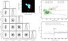 |
Fig. 9 Distance of G043.3+03.1. The red contours refer to the molecular cloud footprint, and the cyan points represent the on-cloud stars. The left and bottom right panels are corner maps and estimate the distance of the MCMC sampling (see Fig. 8 for details). The red and green points in the top right panel present RGs and MSs that were distinguished in the observation data, respectively. The dashed black and red lines show the model-fitted RGs and MSs baseline, respectively. |
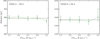 |
Fig. 10 Molecular cloud distances and uncertainties after changing the COcut parameter. The dashed black line is the average of the multiple distances. The left and right panels show the effect of COcut in G045.4-04.2 and G042.9+04.4, respectively. The range of COcut is 3σint to 7σint, where both clouds σint are 0.5. |
5 Summary
We presented a new method for estimating the distances to molecular clouds. As the trial work to evaluate the method, we estimated the distances for 27 molecular clouds using J−Ks colors and the distances provided by 2MASS and Gaia EDR3.
The measured clouds were selected from Yan et al. (2021). For each molecular cloud, we selected on-cloud stars based on the cloud boundary, defined by a certain threshold from the CO map of the MWISP survey. We adopted the stellar populations generated with the TRILEGAL galaxy model as the baseline instead of off-cloud stars. Considering that RGs may affect the distance determination, we distinguished between RGs and MSs for the model and observation data, respectively. The colors of the observation data were calibrated using the corresponding model-fit baseline. Based on the baseline-subtracted data, we successfully used Bayesian analysis and MCMC sampling to estimate the distances of the selected clouds, ranging from ~315 to ~2730 pc. By replacing TRILEGAL with the GALAXIA galaxy model, we measured the distances of 21 clouds using GALAXIA, which are consistent with the distances estimated by TRILEGAL. The typical statistical uncertainties of the distances are ~5%, and the systematic uncertainties from the method are ~1·0%. In the future, we will measure more distances of molecular clouds from the MWISP survey, such as complex regions with indistinguishable molecular cloud boundaries.
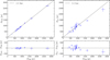 |
Fig. 11 Left panels: comparison between the distances of 21 clouds estimated from the TRILEGAL (DTRI) and GALAXIA (DGAL) models. Right panels: comparison between the distances of the 27 clouds estimated with the TRILEGAL model (DTRI) and those (DLit) of Yan et al. (2021). |
Acknowledgements
This work was supported by the National Natural Science Foundation of China (grants nos. U2031202, 12373030). Z.C. acknowledges the Natural Science Foundation of Jiangsu Province (grants no. BK20231509). This work make use of the data from the Milky Way Imaging Scroll Painting (MWISP) project, which is a multi-line survey in 12CO/13CO/C18O along the northern galactic plane with PMO- 13.7m telescope. We are grateful to all the members of the MWISP working group, particularly the staff members at the PMO 13.7 m telescope, for their long-term support. MWISP is sponsored by the National Key R&D Program of China with grants 2023YFA1608000 and 2017YFA0402701, and the CAS Key Research Program of Frontier Sciences with grant QYZDJ-SSW-SLHO47. This work has made use of data from the European Space Agency (ESA) mission Gaia (https://www.cosmos.esa.int/gaia), processed by the Gaia Data Processing and Analysis Consortium (DPAC, https://www.cosmos.esa.int/web/gaia/dpac/consortium). Funding for the DPAC has been provided by national institutions, in particular the institutions participating in the Gaia Multilateral Agreement. This publication makes use of data products from the Two Micron All Sky Survey, which is a joint project of the University of Massachusetts and the Infrared Processing and Analysis Center/California Institute of Technology, funded by the National Aeronautics and Space Administration and the National Science Foundation.
References
- Andrae, R., Fouesneau, M, Sordo, R., et al. 2023, A&A, 674, A27 [NASA ADS] [CrossRef] [EDP Sciences] [Google Scholar]
- Bailer-Jones, C. A. L., Rybizki, J., Fouesneau, M, Demleitner, M., & Andrae, R. 2021, AJ, 161, 147 [NASA ADS] [CrossRef] [Google Scholar]
- Castro-Ginard, A., McMillan, P. J., Luri, X., et al. 2021, A&A, 652, A162 [NASA ADS] [CrossRef] [EDP Sciences] [Google Scholar]
- Chen, B. Q., Huang, Y., Hou, L. G., et al. 2019, MNRAS, 487, 1400 [NASA ADS] [CrossRef] [Google Scholar]
- Chen, B., Wang, S., Hou, L., et al. 2020a, MNRAS, 496, 4637 [NASA ADS] [CrossRef] [Google Scholar]
- Chen, B. Q., Li, G. X., Yuan, H. B., et al. 2020b, MNRAS, 493, 351 [NASA ADS] [CrossRef] [Google Scholar]
- Chen, Z., Sefako, R., Yang, Y., et al. 2022, Res. Astron. Astrophys., 22, 075017 [CrossRef] [Google Scholar]
- Cutri, R. M., Skrutskie, M. F., van Dyk, S., et al. 2003, VizieR Online Data Catalog: 11/246 [Google Scholar]
- Dame, T. M., Hartmann, D., & Thaddeus, P. 2001, ApJ, 547, 792 [Google Scholar]
- Ester, M., Kriegel, H.-P, Sander, J., & Xu, X. 1996, in Second International Conference on Knowledge Discovery and Data Mning (KDD’96), Proceedings of a conference held August 2–4, 226 [Google Scholar]
- Foreman-Mackey, D., Hogg, D. W., Lang, D., & Goodman, J. 2013, PASP, 125, 306 [Google Scholar]
- Gaia Collaboration (Prusti, L., et al.) 2016, A&A, 595, A1 [NASA ADS] [CrossRef] [EDP Sciences] [Google Scholar]
- Gaia Collaboration (Brown, A. G. A., et al.) 2018, A&A, 616, A1 [NASA ADS] [CrossRef] [EDP Sciences] [Google Scholar]
- Gaia Collaboration (Brown, A. G. A., et al.) 2021, A&A, 649, A1 [NASA ADS] [CrossRef] [EDP Sciences] [Google Scholar]
- Gaia Collaboration (Vallenari, A., et al.) 2023, A&A, 674, A1 [NASA ADS] [CrossRef] [EDP Sciences] [Google Scholar]
- Girardi, L. 2016, Astron. Nachr., 337, 871 [NASA ADS] [CrossRef] [Google Scholar]
- Green, G. M., Schlafly, E. F., Finkbeiner, D. P., et al. 2014, ApJ, 783, 114 [NASA ADS] [CrossRef] [Google Scholar]
- Green, G. M., Schlafly, E., Zucker, C., Speagle, J. S., & Finkbeiner, D. 2019, ApJ, 887, 93 [NASA ADS] [CrossRef] [Google Scholar]
- Guo, H. L., Chen, B. Q., Yuan, H. B., et al. 2021, ApJ, 906, 47 [NASA ADS] [CrossRef] [Google Scholar]
- Guo, H. L., Chen, B. Q., & Liu, X. W. 2022, MNRAS, 511, 2302 [NASA ADS] [CrossRef] [Google Scholar]
- Heyer, M., & Dame, T. M. 2015, ARA&A, 53, 583 [Google Scholar]
- Kennicutt, R. C, & Evans, N. J. 2012, ARA&A, 50, 531 [NASA ADS] [CrossRef] [Google Scholar]
- Kroupa, P. 2002, Science, 295, 82 [Google Scholar]
- Lallement, R., Babusiaux, C., Vergely, J. L., et al. 2019, A&A, 625, A135 [NASA ADS] [CrossRef] [EDP Sciences] [Google Scholar]
- Leike, R., Celli, S., Krone-Martins, A., et al. 2021, Nat. Astron., 5, 832 [NASA ADS] [CrossRef] [Google Scholar]
- Lindegren, L., Hernández, J., Bombrun, A., et al. 2018, A&A, 616, A2 [NASA ADS] [CrossRef] [EDP Sciences] [Google Scholar]
- Lindegren, L., Klioner, S. A., Hernández, J., et al. 2021, A&A, 649, A2 [EDP Sciences] [Google Scholar]
- Magnani, L., Blitz, L., & Mundy, L. 1985, ApJ, 295, 402 [NASA ADS] [CrossRef] [Google Scholar]
- Marton, G., Ábrahám, P., Rimoldini, L., et al. 2023, A&A, 674, A21 [NASA ADS] [CrossRef] [EDP Sciences] [Google Scholar]
- McKee, C. F„ & Ostriker, E. C. 2007, ARA&A, 45, 565 [NASA ADS] [CrossRef] [Google Scholar]
- Reid, M. J., Menten, K. M., Brunthaler, A., et al. 2014, ApJ, 783, 130 [Google Scholar]
- Reid, M. J., Menten, K. M., Brunthaler, A., et al. 2019, ApJ, 885, 131 [Google Scholar]
- Roman-Duval, J., Jackson, J. M., Heyer, M., et al. 2009, ApJ, 699, 1153 [CrossRef] [Google Scholar]
- Russeil, D., Adami, C., & Georgelin, Y. M. 2007, A&A, 470, 161 [NASA ADS] [CrossRef] [EDP Sciences] [Google Scholar]
- Schlafly, E. F., Green, G., Finkbeiner, D. P., et al. 2014, ApJ, 786, 29 [NASA ADS] [CrossRef] [Google Scholar]
- Shan, S.-S., Zhu, H., Tian, W.-W., et al. 2019, Res. Astron. Astrophys., 19, 092 [CrossRef] [Google Scholar]
- Sharma, S., Bland-Hawthorn, J., Johnston, K. V., & Binney, J. 2011, ApJ, 730, 3 [NASA ADS] [CrossRef] [Google Scholar]
- Skrutskie, M. F., Cutri, R. M., Stiening, R., et al. 2006, AJ, 131, 1163 [NASA ADS] [CrossRef] [Google Scholar]
- Su, Y., Yang, J., Zhang, S., et al. 2019, ApJS, 240, 9 [Google Scholar]
- Sun, M., Jiang, B., Yuan, H., & Li, J. 2021a, ApJS, 254, 38 [NASA ADS] [CrossRef] [Google Scholar]
- Sun, M., Jiang, B., Zhao, H., & Ren, Y. 2021b, ApJS, 256, 46 [NASA ADS] [CrossRef] [Google Scholar]
- Wang, S., Zhang, C., Jiang, B., et al. 2020, A&A, 639, A72 [NASA ADS] [CrossRef] [EDP Sciences] [Google Scholar]
- Xu, Y., Reid, M. J., Zheng, X. W., & Menten, K. M. 2006, Science, 311, 54 [NASA ADS] [CrossRef] [Google Scholar]
- Xu, Y., Hou, L.-G., & Wu, Y.-W. 2018, Res. Astron. Astrophys., 18, 146 [CrossRef] [Google Scholar]
- Yan, Q.-Z., Yang, J., Sun, Y., Su, Y., & Xu, Y. 2019, ApJ, 885, 19 [NASA ADS] [CrossRef] [Google Scholar]
- Yan, Q.-Z., Yang, J., Su, Y., Sun, Y., & Wang, C. 2020, ApJ, 898, 80 [CrossRef] [Google Scholar]
- Yan, Q.-Z., Yang, J., Su, Y., et al. 2021, ApJ, 922, 8 [NASA ADS] [CrossRef] [Google Scholar]
- Zhang, M. 2023, ApJS, 265, 59 [NASA ADS] [CrossRef] [Google Scholar]
- Zhao, H., Jiang, B., Li, J., et al. 2020, ApJ, 891, 137 [CrossRef] [Google Scholar]
- Zucker, C., Speagle, J. S., Schlafly, E. F., et al. 2019, ApJ, 879, 125 [NASA ADS] [CrossRef] [Google Scholar]
- Zucker, C., Speagle, J. S., Schlafly, E. F., et al. 2020, A&A, 633, A51 [NASA ADS] [CrossRef] [EDP Sciences] [Google Scholar]
All Tables
All Figures
|
Fig. 1 Left panel: selected on-cloud stars for G045.1-03.4. The red contour shows the molecular cloud footprint, and the cyan points represent on-cloud stars. Right panel: J−Ks color vs. distance diagram. It has two branches. |
| In the text | |
|
Fig. 2 Left and right panels: J−Ks color vs. distance and GBP − GRP color vs. distance diagram for G045.1-03.4, respectively. The purple squares represent the model data, and the black points represent the observation data. |
| In the text | |
|
Fig. 3 Ks vs. J−Ks diagram of the observation and model data for G045.1-03.4. The squares represent the model data, the hollow circles represent the observation data, and the color represents the distance. The dashed black line is Ks = 14 mag. |
| In the text | |
|
Fig. 4 Distributions of the observation and model data in the color-distance diagram for G045.1-03.4. The purple squares represent the model data, the colored points represent the observation data with log g, and the black points represent the observation data without log g. |
| In the text | |
|
Fig. 5 Left and right panels: fit baselines for MSs (dashed black line) and for RGs (dashed red line) in the model data, respectively. The gray squares present the model data. The green and orange squares present the binned MSs and RGs stars (every 50 pc), respectively. |
| In the text | |
|
Fig. 6 Left panel: distinguished MSs and RGs in the observation data using the 3σ lower bound line of the model-fit RGs baseline (dashed purple line) and a distance of 1 kpc. Right panel: further distinction between the RGs and reddened stars for the differentiated RGs, and reddened stars are classified as MSs. The green and red points show the MSs and RGs of the observation data, respectively. |
| In the text | |
|
Fig. 7 Distribution of the observation data after the color is calibrated. The gray points present the baseline-subtracted observation data. The blue points plot the mean color of the binned stars (every 50 pc for the distance), which are only used to confirm the results for inspection by eye and not to calculate the distance. |
| In the text | |
|
Fig. 8 Distances of GO45.1-03.4. The corner plots of the MCMC samples of five modeled parameters and their uncertainties are displayed on the left. The right panel displays the distance result. The vertical black lines indicate the estimated distance (D), and the shadow areas depict the 16th and 84th percentile values of the cloud distance. The broken horizontal dashed purple line is the color variation of the on-cloud stars after the baseline was subtracted. |
| In the text | |
|
Fig. 9 Distance of G043.3+03.1. The red contours refer to the molecular cloud footprint, and the cyan points represent the on-cloud stars. The left and bottom right panels are corner maps and estimate the distance of the MCMC sampling (see Fig. 8 for details). The red and green points in the top right panel present RGs and MSs that were distinguished in the observation data, respectively. The dashed black and red lines show the model-fitted RGs and MSs baseline, respectively. |
| In the text | |
|
Fig. 10 Molecular cloud distances and uncertainties after changing the COcut parameter. The dashed black line is the average of the multiple distances. The left and right panels show the effect of COcut in G045.4-04.2 and G042.9+04.4, respectively. The range of COcut is 3σint to 7σint, where both clouds σint are 0.5. |
| In the text | |
|
Fig. 11 Left panels: comparison between the distances of 21 clouds estimated from the TRILEGAL (DTRI) and GALAXIA (DGAL) models. Right panels: comparison between the distances of the 27 clouds estimated with the TRILEGAL model (DTRI) and those (DLit) of Yan et al. (2021). |
| In the text | |
Current usage metrics show cumulative count of Article Views (full-text article views including HTML views, PDF and ePub downloads, according to the available data) and Abstracts Views on Vision4Press platform.
Data correspond to usage on the plateform after 2015. The current usage metrics is available 48-96 hours after online publication and is updated daily on week days.
Initial download of the metrics may take a while.