| Issue |
A&A
Volume 684, April 2024
|
|
|---|---|---|
| Article Number | A100 | |
| Number of page(s) | 13 | |
| Section | Cosmology (including clusters of galaxies) | |
| DOI | https://doi.org/10.1051/0004-6361/202347929 | |
| Published online | 11 April 2024 | |
Bayesian deep learning for cosmic volumes with modified gravity
1
Instituto de Astrofísica de Canarias, s/n, 38205 La Laguna, Tenerife, Spain
e-mail: jorge.farieta@iac.es
2
Departamento de Astrofísica, Universidad de La Laguna, 38206 La Laguna, Tenerife, Spain
3
Grupo Signos, Departamento de Matemáticas, Universidad El Bosque, Bogotá, Colombia
e-mail: hhortuao@unbosque.edu.co
4
Maestría en Ciencia de Datos, Universidad Escuela Colombiana de Ingeniería Julio Garavito, Bogotá, Colombia
Received:
10
September
2023
Accepted:
24
January
2024
Context. The new generation of galaxy surveys will provide unprecedented data that will allow us to test gravity deviations at cosmological scales at a much higher precision than could be achieved previously. A robust cosmological analysis of the large-scale structure demands exploiting the nonlinear information encoded in the cosmic web. Machine-learning techniques provide these tools, but no a priori assessment of the uncertainties.
Aims. We extract cosmological parameters from modified gravity (MG) simulations through deep neural networks that include uncertainty estimations.
Methods. We implemented Bayesian neural networks (BNNs) with an enriched approximate posterior distribution considering two cases: the first case with a single Bayesian last layer (BLL), and the other case with Bayesian layers at all levels (FullB). We trained both BNNs with real-space density fields and power spectra from a suite of 2000 dark matter-only particle-mesh N-body simulations including MG models relying on MG-PICOLA, covering 256 h−1 Mpc side cubical volumes with 1283 particles.
Results. BNNs excel in accurately predicting parameters for Ωm and σ8 and their respective correlation with the MG parameter. Furthermore, we find that BNNs yield well-calibrated uncertainty estimates that overcome the over- and under-estimation issues in traditional neural networks. The MG parameter leads to a significant degeneracy, and σ8 might be one possible explanation of the poor MG predictions. Ignoring MG, we obtain a deviation of the relative errors in Ωm and σ8 by 30% at least. Moreover, we report consistent results from the density field and power spectrum analysis and comparable results between BLL and FullB experiments. This halved the computing time. This work contributes to preparing the path for extracting cosmological parameters from complete small cosmic volumes towards the highly nonlinear regime.
Key words: methods: data analysis / methods: numerical / methods: statistical / cosmological parameters / large-scale structure of Universe
© The Authors 2024
 Open Access article, published by EDP Sciences, under the terms of the Creative Commons Attribution License (https://creativecommons.org/licenses/by/4.0), which permits unrestricted use, distribution, and reproduction in any medium, provided the original work is properly cited.
This article is published in open access under the Subscribe to Open model. Subscribe to A&A to support open access publication.
1. Introduction
Cosmic acceleration is one of the most critical concerns in modern cosmology. In the context of the concordance model ΛCDM (Λ cold dark matter), this acceleration is attributed to the existence of a fluid with negative pressure that is represented by the cosmological constant, Λ, in general relativity (GR) equations. However, this fluid introduces some conceptual and theoretical issues that have not been fully addressed, either observationally or theoretically. Alternative theories, such as MG models, have attracted attention as a natural explanation for cosmic acceleration without invoking a cosmological constant (see, e.g., Nojiri et al. 2017, for a recent review). Among the plethora of alternative models, some parametrisations of f(R) gravity have gained popularity because they can accurately reproduce the standard model predictions. The two cosmological scenarios ΛCDM and f(R) are indeed highly successful in providing an accurate description of the Universe on large scales, from cosmic microwave background (CMB) observations to the data of galaxy clustering (Berti et al. 2015).
Unlike the standard scenario, the f(R) models do not require a cosmological constant, but instead modify the behaviour of gravity itself. The modification of Einstein’s GR involves the addition of a scalar field that emulates cosmic acceleration. This feature of f(R) models has made them perfect templates for tracking departures from standard gravity. Consequently, a crucial task within the scope of precision cosmology is to quantify the potential variations in gravity using appropriate techniques that are sensitive to MG effects. Some of the approaches to achieve this aim include using clustering anisotropies (Jennings et al. 2012; García-Farieta et al. 2019, 2020; Hernández-Aguayo et al. 2019), tracer bias and sample selection (García-Farieta et al. 2021), cosmic voids (Voivodic et al. 2017; Perico et al. 2019; Contarini et al. 2021), halo mass functions (Hagstotz et al. 2019; Gupta et al. 2022), and peculiar velocities (Johnson et al. 2016; Ivarsen et al. 2016; Lyall et al. 2023).
The matter distribution is a rich source of cosmological information that has been exploited for many years through various techniques. One of the most frequently used techniques to extract information from the large-scale structure (LSS) data relies on the two-point statistics as described by the two-point correlation function or its equivalent in Fourier space, the matter power spectrum. Despite its success in capturing all possible cosmological information contained in a density field, it fails to capture features affected by the non-Gaussian nature of density perturbations, and its accuracy and precision cannot be relied upon for probing small angular scales. Since the estimators up to second order do not contain all cosmological information, other techniques beyond the two-point statistics have been studied to extract additional information, such as N-point correlation functions (Peebles 2001; Takada & Jain 2003; Zhang et al. 2022; Brown et al. 2022; Veropalumbo et al. 2022; Philcox et al. 2022), Minkowski functionals (Kratochvil et al. 2012; Hikage et al. 2003; Fang et al. 2017), peak count statistics (Kacprzak et al. 2016; Peel et al. 2017; Fluri et al. 2018; Harnois-Déraps et al. 2021), density split statistics (Paillas et al. 2021), cosmic shear (Kilbinger 2015; Van Waerbeke et al. 2001), cosmic voids (Cai et al. 2015; Bos et al. 2012; Hamaus et al. 2016; Lavaux & Wandelt 2010), and tomographic analyses based on the Alcock-Paczynski test (Park & Kim 2010; Zhang et al. 2019; Li et al. 2015; Luo et al. 2019; Dong et al. 2023), and Bayesian inference (Nguyen et al. 2023; Kostić et al. 2023). For an overview of contemporary cosmological probes, we refer to Weinberg et al. (2013) and Moresco et al. (2022).
Recently, deep neural networks (DNNs) have been proposed as a new alternative for not only recollecting the three-dimensional (3D) density field information without specifying the summary statistic beforehand, such as the power spectrum, but also for managing the demanding computational needs in astrophysics (Dvorkin et al. 2022). The method involving parameter inference and model comparison directly from simulations, that is, using high-dimensional data, is formally termed simulation-based inference (Thomas et al. 2016; Lemos et al. 2023a,b; Hahn et al. 2022). This technique is sometimes referred to as approximate Bayesian computation, implicit likelihood inference, or non-likelihood inference (Csilléry et al. 2010; Sunnåker et al. 2013; Beaumont 2010). The CNN algorithms have been explored as a valuable tool in MG scenarios, mainly with applications in weak-lensing maps such as emulator building (Tamosiunas et al. 2021) and also to investigate observational degeneracies between MG models and massive neutrinos (Merten et al. 2019; Peel et al. 2019), CMB patch map analysis (Hortúa et al. 2020a), and N-body simulations (Lazanu 2021; Alves de Oliveira et al. 2020; Kodi Ramanah et al. 2020). Bayesian neural networks (BNNs) have also been employed to identify and classify power spectra that deviate from ΛCDM such as MG models, however (Mancarella et al. 2022).
Even though they can extract information from complex data, standard DNNs still overfit or memorise noisy labels during the training phase, and their point estimates are not always reliable. BNNs are extensions of DNNs that provide probabilistic properties on their outcomes and yield predictive uncertainties (Denker & LeCun 1990; Gal & Ghahramani 2016). Some BBN approaches include stochastic MCMC (Deng et al. 2019), Bayes by backprop (Blundell et al. 2015), deep ensembles (Lakshminarayanan et al. 2017), or Monte Carlo dropout and flipout (Gal 2016; Wen et al. 2018). Other BNN alternatives employ variational inference (VI) to infer posterior distributions for the network weights that are suitable to capture its uncertainties, which are propagated to the network output (Graves 2011; Gunapati et al. 2022). Although VI speeds up the computation of the posterior distribution when analytic approaches are considered, these assumptions can also introduce a bias (Charnock et al. 2022) that yields overconfident uncertainty predictions and significant deviations from the true posterior. Hortúa et al. (2020b) and Hortua (2021) added normalising flows on top of BNNs to give the joint parameter distribution more flexibility. However, this approach was not implemented into the Bayesian framework, so that the bias is still preserved. In a recent work (Hortúa et al. 2023), the authors improved the previous method by applying multiplicative normalising flows, which resulted in accurate uncertainty estimates. In this paper, we follow the same approach by building BNN models adapted to both 3D density field and its power spectra to constrain MG from cosmological simulations. We show that for non-Gaussian signals alone, it is possible to improve the posterior distributions, and when the additional information from the power spectrum is considered, they yield more significant performance improvements without underestimating the posterior distributions. The analysis focuses on simulated dark matter fields from cosmological models beyond ΛCDM to assess whether the inference schemes can reliably capture as much information as possible from the nonlinear regime. However, the applicability of the proposed model can be adapted to be easily used with small-volume mock galaxy catalogues. This paper is organised as follows. Section 2 offers a summary of structure formation in MG cosmologies and the reference simulations we created to train and test the BNNs. In Sect. 3 we briefly introduce the BNN concept, and Sect. 4 shows the architectures and configuration we used in the paper. The results are presented in Sect. 5, and an extended discussion of the findings is presented in Sect. 6. Our conclusions are given in Sect. 7.
2. Large-scale structure in modified gravity
In this section, we present the gravity model that coincides with ΛCDM in the limiting case of a vanishing f(R) parameter introduced below.
2.1. Structure formation and background
In f(R) cosmologies, the dynamics of matter is determined by the modified Einstein field equations. The most straightforward modification of GR that circumvents Λ emerges by including a function of the curvature scalar in the Einstein-Hilbert action. In this modification, the equations of motion are enriched with a term that depends on the curvature scalar and that creates the same effect as dark energy (for a review on different MG models see e.g. Tsujikawa et al. 2008; De Felice & Tsujikawa 2010). For consistency across various cosmological scales, Hu & Sawicki (2007, hereafter HS) proposed a viable f(R) function that can satisfy tight constraints at Solar System scales and that also accurately describes the dynamics of the ΛCDM background. In these models, the modified Einstein-Hilbert action is given by
![$$ \begin{aligned} S_{\rm EH}=\int \mathrm{d}^4 x \sqrt{-g}\left[\frac{R+f(R)}{16 \pi G}\right], \end{aligned} $$](/articles/aa/full_html/2024/04/aa47929-23/aa47929-23-eq1.gif)
where g is the metric tensor, G is Newton’s gravitational constant, R is the curvature scalar, and f(R) is a scalar function that constrains the additional degree of freedom. In the HS model, this function takes the form
where n, c1, and c2 are model parameters, and  , with Ωm being the current fractional matter density, and H0 is the Hubble parameter at the present time. For n = 1, which is the f(R) model we consider in this paper, the function can be written as follows:
Here, fR0 represents the dimensionless scalar field at the present time, meaning the only additional degree of freedom that stems from the derivative of f(R) with respect to the curvature scalar, fR. The modified Einstein field equations and analogous Friedmann equations that describe the HS model background can be obtained from minimising the action (for a thorough derivation see Song et al. 2007). To further understand the formation and evolution of large-scale structures in MG, it is crucial to describe the matter perturbations, δm, around the background (see Song et al. 2007). The MG effects are captured by the growth of density perturbations in the matter-dominated era when the mildly nonlinear regime is important (Laszlo & Bean 2008). In particular, when considering linear perturbations, the equations of the evolution of matter overdensities in Fourier space are as follows (Tsujikawa 2008):
![$$ \begin{aligned} \begin{aligned}&\ddot{\delta }_{\rm m}+\left(2 H+\frac{\dot{F}}{2 F}\right) \dot{\delta }_{\rm m}-\frac{\rho _{\rm m}}{2 F} \delta _{\rm m} \\&\qquad =\frac{1}{2 F}\left[\left(-6 H^2+\frac{k^2}{a^2}\right) \delta F+3 H \delta \dot{F}+3 \delta \ddot{F}\right], \\&\delta \ddot{F}+3 H \delta \dot{F}+\left(\frac{k^2}{a^2}+\frac{F}{3 F_R}-4 H^2-2 \dot{H}\right) \delta F\\&\qquad =\frac{1}{3} \delta \rho _{\rm m}+\dot{F} \dot{\delta }_{\rm m}, \end{aligned} \end{aligned} $$](/articles/aa/full_html/2024/04/aa47929-23/aa47929-23-eq5.gif)
with H being the Hubble parameter, k the comoving wavenumber of the perturbations, a the scale factor, ρm the matter density field, and F ≡ ∂f/∂R. The solution to the system of Eq. (4) provides a detailed description of δm, which includes most of the cosmological information since it is a direct result of the gravitational interaction of cosmic structures. To obtain insights into the underlying cosmic parameters, the density field is the primary source to be investigated using summary statistics. The Eq. (4) make evident the connection between the density field and the scalaron of MG. Consequently, any departure from GR would be measurable through the density field, either with the structure growth rate, or with its tracer distribution. A particular feature of the f(R) models is the so-called chameleon mechanism. This mechanism reconciles the departures of GR with the bounds imposed by local tests of gravity. It gives the mass of the scalar field the ability to depend on the local matter density. More precisely, the signatures of MG can be detected in regions of lower matter density where the scalar field becomes lighter, leading to potentially observable effects that deviate from standard gravity (Odintsov et al. 2023).
The 3D matter power spectrum, denoted P(k), is a primary statistical tool employed to extract cosmological insights from the density field. It characterises the overdensities as a function of scale and is estimated through the following average over Fourier space:

where  is the 3D Dirac-delta function. This function contains all the information from the statistics of the density field in the linear regime and a decreasing fraction of the total information on smaller scales when the initial density fields follow Gaussian statistics. We used the Pylians31 library to estimate the overdensity field as well as the power spectrum.
2.2. Modified-gravity simulations
The simulations were created with the COmoving Lagrangian Acceleration (COLA) algorithm (Tassev et al. 2013; Koda et al. 2016), which is based on a particle-mesh code that solves the equations of motion following the Lagrangian perturbation theory (LPT) trajectories of the particles. This algorithm speeds up the computation of the gravitational force using very few time steps and still obtains correct results on the largest scales. In particular, we used MG-PICOLA2 (Winther et al. 2017), a modified version of L-PICOLA (Howlett et al. 2015) that has been extensively tested against full N-body simulations and that extends the gravity solvers to MG models, including the HS parametrisation.
We ran a set of 2500 MG simulations for which we varied the four cosmological parameters Θ = {Ωm, h, σ8, fR0}, where h is the reduced Hubble parameter, σ8 is the rms density fluctuation within a top-hat sphere with a radius of 8 h−1 Mpc, and fR0 is the amplitude of the MG function in the HS model. The remaining cosmological parameters were set to Ωb = 0.048206 and ns = 0.96, which correspond to the values reported by Planck Collaboration VI (2020). The parameter space was sampled with random numbers uniformly distributed within the specified ranges for each parameter (see Table 1). Since the typical values of the MG parameter go as powers of ten, |fR0|∼10n with n ∈ [ − 4, −6], we chose to sample a fraction of its logarithm in order to cover the range of powers equally, that is,  . Figure 1 illustrates the parameter space variations of the 2500 MG cosmologies, each of which is represented by a grey line. The values of the cosmological parameters, Θ, are distributed along the different vertical axes. Each simulation follows the dynamics of 1283 particles in a small box with a comoving side-length of 256 h−1 Mpc using 100 time steps from an initial redshift zi = 49 up to redshift z = 0. This simulation resolution allows us to reasonably investigate the impacts of MG on large scales, in particular for the fR0 values considered in this work. However, it is not as effective at very small scales, where a higher resolution is required. MG solvers have undergone extensive testing using low-resolution simulations (see e.g. Puchwein et al. 2013; Li et al. 2012; Hernández-Aguayo et al. 2022). These tests show the enhancement of the power spectrum in simulations of 256 h−1 Mpc, where MG effects begin to be seen. Our setup of the MG simulations is summarised in Table 1. In a recent research, a similar setup was employed with a light-weight deterministic CNN to estimate a subset of parameters of a flat ΛCDM cosmology (Pan et al. 2020), but we chose a time-step that is larger by a factor of 2.5. The initial conditions for the MG simulations were created with 2LPTic (Crocce et al. 2006, 2012) based on a ΛCDM template at zi. Moreover, a distinct random seed was assigned to each simulation to generate varying distributions of large-scale power. This approach allowed our neural network to effectively capture the inherent cosmic variance.
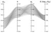 |
Fig. 1. Multidimensional parameter space variations. Each line represents the parameter values of a data point. The four parameters Ωm, h, σ8, and 0.1log10|fR0| are visualised along separate axes. |
Summary of the setup of the MG simulations.
We calculated the overdensity field, δm, for each snapshot at redshift z = 0 employing the cloud-in-cell (CIC) mass-assignment scheme (Hockney & Eastwood 1981) on a regular grid consisting of N3 = 1283 voxels. The training set comprised 80% of the data, which corresponds to 2000 boxes containing the overdensity fields, while the remaining 20% of the data were used for testing. Figure 2 displays the 3D overdensity field plus the unity,  , projected along each plane of the box. The displayed data correspond to an arbitrarily chosen combination of parameters within the MG simulation suite at redshift z = 0. Similarly, Fig. 3 displays the 2D density field of dark matter in a region of 256 × 256 × 20 (h−1 Mpc)3 from 100 out of 2500 arbitrarily chosen simulations of MG. The cosmological parameter combination is indicated by the labels. The cuts in the density field provide a visual means to discern distinct features of the cosmic web that are observable with the naked eye. These features include variations in the filament structure of the cosmic web, which become evident in the zones of under- and over-densities. Additionally, we output the matter power spectrum of all realisations by directly computing the modulus of each Fourier mode from the particle distribution, |δm(k)|2. The Fig. 4 shows the different matter power spectra for the entire MG simulation suit. The variations in the shape of the spectrum correspond to the joint effect of cosmological parameters that were varied as shown in the label. We considered the effective range of the power spectrum up to the Nyquist frequency, kNy, which in our simulations corresponds to k ≈ 1.58 Mpc h−1. The full datasets used in this paper, 3D overdensity fields as well as power spectra, are publicly available in Zenodo3.
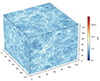 |
Fig. 2. Projected overdensity field at redshift z = 0 derived from an arbitrarily chosen simulation within the ensemble of 2500 MG simulations. The normalised density field was calculated using a CIC mass-assignment scheme. |
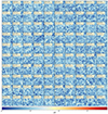 |
Fig. 3. Projected density field of dark matter in a region of 256 × 256 × 20 (h−1 Mpc)3 from 100 out of 2500 arbitrarily chosen simulations of MG. The snapshots are taken at z = 0, and the legend displays the set of cosmological parameters of {Ωm, h, σ8, fR0}. The cuts in the density field highlight the broad coverage of the parameter space of the MG simulations. Different features can be observed by naked eye, such as variations in the filament structure of the cosmic web. |
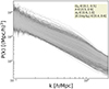 |
Fig. 4. Matter power spectrum at z = 0 of the MG simulation suit. The variations in the spectrum correspond to changes in each of the four parameters that were varied, Ωm, h, σ8 and |0.1 log fR0|. The corresponding range of each of parameter is shown in the label. |
3. Bayesian neural networks
The primary goal of BNNs is to estimate the posterior distribution p(w|𝒟), which represents the probability distribution of the weights w of the network given the observed data 𝒟 = (X, Y) (Abdar et al. 2021; Gal 2016; Graves 2011). The posterior distribution, denoted as p(w|𝒟), can be derived using Bayes’ law: p(w|𝒟)∼p(𝒟|w)p(w). This expression involves a likelihood function, p(𝒟|w), which represents the probability of the observed data 𝒟 given the weights w, as well as a prior distribution on the weights, denoted as p(w). After the computation of the posterior, the probability distribution of a new test example x* can be determined by
where p(y*|x*, w) is the predictive distribution corresponding to the set of weights. In the context of neural networks, it is important to note that the direct computation of the posterior is not feasible (Gal 2016). To circumvent this limitation, variational inference (VI) techniques approximating the posterior distribution were introduced (Graves 2011). VI considers a family of simple distributions, denoted as q(w|θ), which is characterised by a parameter θ. The objective of VI is to identify a distribution q(w|θ*) that minimises the Kullback–Leibler divergence between q(w|θ) and p(w|𝒟), where θ* represents the optimal parameter values, and KL[ ⋅ ∥ ⋅ ] is the Kullback–Leibler divergence. This optimisation is equivalent to maximising the evidence lower bound (ELBO; Gal 2016),
![$$ \begin{aligned} \mathrm{ELBO}(\theta ) = {\mathbb{E} }_{q({ w}|\theta )}\big [\log p(Y|X,{ w})\big ] - \mathrm{KL}\big [q({ w}|\theta )\big \Vert p({ w})\big ], \end{aligned} $$](/articles/aa/full_html/2024/04/aa47929-23/aa47929-23-eq11.gif)
where 𝔼q(w|θ)[log p(Y|X, w)] is the expected log-likelihood with respect to the variational posterior and KL[q(w|θ)||p(w)] is the divergence of the variational posterior from the prior. Equation (7) shows that the Kullback–Leibler (KL) divergence serves as regulariser, compelling the variational posterior to shift towards the modes of the prior. A frequently employed option for the variational posterior entails using a product of independent Gaussian distributions, specifically, mean-field Gaussian distributions. Each parameter w is associated with its own distribution (Abdar et al. 2021),
where i and j are the indices of the neurons from the previous and current layers, respectively. Applying the reparametrisation trick, we obtained wij = μij + σij * ϵij, where ϵij was drawn from the normal distribution. Moreover, when the prior is a composition of independent Gaussian distributions, the KL-divergence between the prior and the variational posterior can be calculated analytically. This characteristic enhances the computing efficiency of this approach.
3.1. Multiplicative normalising flows
The Gaussian mean-field distributions described in Eq. (8) are the most commonly used family for the variational posterior in BNNs. Unfortunately, this distribution lacks the capacity to adequately represent the intricate nature of the true posterior. Hence, it is anticipated that enhancing the complexity of the variational posterior will yield substantial improvements in performance. This is attributed to the capability of sampling from a more reliable distribution, which closely approximates the true posterior distribution. The process of improving the variational posterior demands efficient computational methods while ensuring its numerical feasibility. Multiplicative normalising flows (MNFs) have been proposed to efficiently adapt the posterior distributions by using auxiliary random variables and the normalising flows (Louizos & Welling 2017). Mixture normalising flows (MNFs) suggest that the variational posterior can be mathematically represented as an infinite mixture of distributions,
with θ the learnable posterior parameter, and z ∼ q(z|θ)≡q(z)4 the vector with the same dimension as the input layer, which plays the role of an auxiliary latent variable. Moreover, allowing for local reparametrisations, the variational posterior for fully connected layers becomes
Here, we can increase the flexibility of the variational posterior by enhancing the complexity of q(z). This can be done using normalising flows since the dimensionality of z is much lower than the weights. Starting from samples z0 ∼ q(z0) from fully factorised Gaussians (see Eq. (8)), a rich distribution q(zK) can be obtained by applying successively invertible fk-transformations,

To handle the intractability of the posterior, Louizos & Welling (2017) suggested to use again Bayes law q(zK)q(w|zK) = q(w)q(zK|w) and introduce a new auxiliary distribution r(zK|w, ϕ) parametrised by ϕ, with the purpose of approximating the posterior distribution of the original variational parameters q(zK|w) to further lower the bound of the KL divergence term. Accordingly, the KL-divergence term can be rewritten as follows:
![$$ \begin{aligned} -\mathrm{KL}\big [q({ w})\big \Vert p({ w})\big ]&\ge {\mathbb{E} }_{q({ w},z_K)}\biggl [-\mathrm{KL}\big [q({ w}|z_K)\big \Vert p({ w})\big ]\biggr .\nonumber \\&\biggl . +\log q(z_K)+\log r(z_K|{ w},\phi )\biggr ]. \end{aligned} $$](/articles/aa/full_html/2024/04/aa47929-23/aa47929-23-eq17.gif)
The first term can be analytically computed since it will be the KL-divergence between two Gaussian distributions, while
Input: feature vector of the previous layer (minibatch)
H ← Input conv3D-layer (minibatch)
z0 ∼ q(z0)
zTf = NF(z0)
Mh = H ∗ (Mw ⊙ reshape(zTf, [1, 1, 1, Df]))
Vh = H2 ∗ Σw
E ∼ 𝒩(0; 1)
return Mh +  ⊙ E
⊙ E
Output: sample of feature vector according to Eq. (17)
the second term is computed via the normalising flow generated by fK (see Eq. (12)). Furthermore, the auxiliary posterior term is parametrised by inverse normalising flows as follows (Touati et al. 2018):

and
where  can be parametrised as another normalising flow. A flexible parametrisation of the auxiliary posterior can be given by
where the parameterisation of the mean  , and the variance
  is carried out by the masked RealNVP (Dinh et al. 2017) as the choice of normalising flows.
3.2. Multiplicative normalising flows in a voxel-grid representation
In this section, we present our first result, where we have generalised Eq. (10) to 3D convolutional layers where cosmological simulated data are structured. To this end, we started with the extension of sampling from the variational posterior as
where Dh, Dw, and Dd are the three spatial dimensions of the boxes, and Df is the number of filters for each kernel. The objective is to address the challenge of enhancing the adaptability of the approximate posterior distribution for the weight coming from a 3D convolutional layer. Algorithm 1 outlines the procedure to forward propagation for each 3D convolutional layer. Similar to the fully connected case, the auxiliary parameter only affects the mean with the purpose of avoiding large variance, and we kept a linear mapping to parameterise the inverse normalising flows instead of applying tanh feature transformations.
4. The Bayesian architecture setup
We examined four distinct architectures of BNNs, as outlined in Sect. 3. Two of these architectures include Bayesian layers located only on top of the network, the so-called Bayesian last layer (denoted as BLL), while the remainder have Bayesian layers at all their levels (FullB). The pipelines used in our study were developed using TensorFlow v:2.125 and TensorFlow-probability v:0.196 (Abadi et al. 2016). The architecture used for all networks has ResNet-18 as the backbone, which is depicted in a schematic manner in Table 2. The input layer receives simulated boxes of (128, 128, 128, 1) with normalised voxels in the range 0−1. The Resblock nature depends on whether we build a ResNet or an SeResNet topology. The latter is a variant of ResNet that employs squeeze-and-excitation blocks that adaptively re-calibrate channel-wise feature responses by explicitly modelling inter-dependences between channels (Hu et al. 2017). Figure 5 depicts each Resblock and how the skip connections are defined. These architectures were designed using the GIT repository classification-models-3D7. ResNet18 contains 2510149 trainable parameters while SeResNet has 3069270, but these numbers are duplicates in a fully Bayesian scheme because two parameters need to be optimised (the mean and standard deviation) for each network parameter. In this study, 50 layers were employed for the masked RealNVP normalising flow. The development of these convolutional layers was made using the repositories TF-MNF-VBNN8 and MNF-VBNN9 as well (Louizos & Welling 2017). Finally, all networks end with a multivariate Gaussian distribution layer, consisting of 14 trainable parameters. These parameters include four means, denoted as μ, which correspond to the cosmological parameters, as well as ten elements representing the covariance matrix Σ. TensorFlow probability has a built-in version of the multivariate normal distribution, MultivariateNormalTriL, that is parametrised in terms of the Cholesky factor of the covariance matrix. This decomposition guarantees the positiveness of the covariance matrix. In addition, we included a reparametrisation led by ReLU activation to force positive values in the mean of the distribution. The loss function to be optimised is given by the ELBO, Eq. (7), where the second term is associated with the negative log-likelihood (NLL),
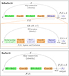 |
Fig. 5. Resblock schema depending on the architecture used. Top: resblock when SeResNet18 is employed. The dashed orange rectangle shows the skip SE-connection schema used in the SeResNet18 resblock. Bottom: resblock when ResNet is employed. |
Configuration of the (Se)-ResNet backbone used for all experiments presented in this paper.
averaged over the mini-batch. The optimiser used was an Adam optimiser with first- and second-moment exponential decay rates of 0.9 and 0.999, respectively (Kingma & Ba 2014). The learning rate started from 5 × 10⁻⁴ and was reduced by a factor of 0.9 when no improvement was observed after 8 epochs. Furthermore, we applied a warm-up period for which the model progressively turned on the KL term in Eq. (7). This was achieved by introducing a β variable in the ELBO, that is, β ⋅ KL[q(w|θ)∥p(w)], so that this parameter started being equal to 0 and grew linearly to 1 during 12 epochs (Sønderby et al. 2016). BNNs were trained with a batch size of 8, and early-stopping callback was presented to avoid overfitting. Finally, hyperparameter tuning was applied to the filters (the initial filters were 64, 32, and 16, after which they increased as 2n, where n stands for the number of layers) in the convolutional layers for ResNet (18, 32, 50), SeResNet (18, 32, 50), VGG (16, 19), and MobileNet. The infrastructure set in place by the Google Cloud Platform10 (GCP) uses an nvidia-tesla-t4 of 16 GB GDDR6 in an N1 machine-series shared-core.
Quantifying the performance
The metrics employed for determining the network performance were the mean square error (MSE), ELBO, and the coefficient of the determination r2. Moreover, we quantified the quality of the uncertainty estimates through reliability metrics. Following Laves et al. (2020) and Guo et al. (2017), we defined a perfect calibration of the regression uncertainty as
![$$ \begin{aligned} \mathbb{E} _{\hat{\sigma }^{2}} \left[ \mathrm{abs}\big [\big ( ||\boldsymbol{y}-\boldsymbol{\mu }||^2 \, \big | \, \hat{\sigma }^{2} = \alpha ^{2} \big ) - \alpha ^{2} \big ] \right] \quad \forall \left\{ \alpha ^{2} \in \mathbb{R} \, \big | \, \alpha ^{2} \ge 0 \right\} , \end{aligned} $$](/articles/aa/full_html/2024/04/aa47929-23/aa47929-23-eq31.gif)
where abs[.] is the absolute value function. The predicted uncertainty  was partitioned into K bins with equal width in this way, and the variance per bin is defined as
with N stochastic forward passes. In addition, the uncertainty per bin is defined as
which allowed us to compute the expected uncertainty calibration error (UCE) in order to quantify the miscalibration,
with the number of inputs m and set of indices Bk of inputs, for which the uncertainty falls into bin k.
5. Results
In this section, we present the results of several experiments we developed to quantify the performance of Bayesian deep-learning neural networks for constraining the cosmological parameters in MG scenarios.
5.1. Parameter estimation from the overdensity field under a voxel-grid representation
Using the configuration described in Sect. 4, we designed four experiments inspired by two successful deep-learning architectures, ResNet18 and Se-ResNet18. The former is a residual network commonly known due to its efficiency in several computer vision tasks, while the latter was chosen because of its ability to improve the interdependences between the channels of convolutional feature layers (Hu et al. 2017). Furthermore, the modification of the models was also based on the insertion of a set of Bayesian layers at either the top of the model (BLL) or in the entire architecture (FullB). The motivation for exploring both possibilities comes from the fact that intuitively, adding a Bayesian layer at the end of the network (BLL) can be viewed as Bayesian linear regression with a learnable projected feature space, allowing for a successful balance between scalability and the degree of model agnosticism (Fiedler & Lucia 2023; Watson et al. 2021). Conversely, although fully Bayesian networks (FullB) would demand high computational resources, it has been reported that their Bayesian hidden layers are susceptible to out-of-distribution (OOD) examples that might improve the predictive uncertainty estimates (Henning et al. 2021). The results of the experiments performed in this work are summarised in Table 3. It shows the performance of each architecture on the test set. In the top part of the table, the results of the SeResNet18 topology are shown, and in the bottom part, the results of ResNet18 are presented. The left columns of the table correspond to the FullB scheme, and the left colum corresponds to the Bayesian last layer, BLL. Comparing all approaches, we observe that FullB-SeResNet18 slightly outperforms the rest of the models in terms of accuracy (described by r2) and uncertainty quality provided by UCE. However, no significant differences were found in the reported metrics for ResNet and its SeResNet counterpart, except for the inference time, where the BLL models clearly outperform the FullB models. This suggests that FullBs yield small improvements in the computation of the uncertainties at the expense of duplicating the inference time. In addition, both architectures estimate σ8 more efficiently than for any other parameter, especially in contrast to h or 0.1log10|fR0|, although the FullBs respond slightly better to MG effects. Figure 6 displays the scatter relation between the predicted and ground-truth values of each cosmological parameter using FullB-SeResNet18. It also shows the degeneracy directions that arise from observations defined as Ωmh2 and  (this parameter combination was taken from Planck and CMB lensing McCarthy et al. 2023). The diagonal grey lines correspond to the ideal case of a perfect parameter prediction. Each data point represents the mean value of the predicted distributions, and the error bars stand for the heteroscedastic uncertainty associated with epistemic plus aleatoric uncertainty at 1σ confidence level. As we observe, BNNs learn how to accurately predict the value for Ωm and σ8, but they fail to capture information related to the MG effects and the Hubble parameter. Even though parameter estimation derives from all features of the fully nonlinear 3D overdensity field, the horizontal scatter pattern that exhibits the Hubble and MG parameters implies that essential underlying connections are not effectively captured. A similar result for the Hubble parameter using DCNNs in ΛCDM can be found in Villaescusa-Navarro et al. (2020).
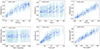 |
Fig. 6. True vs. predicted values provided by the FullB model for Ωm, σ8, and some derivative parameters. The points are the mean of the predicted distributions, and the error bars stand for the heteroscedastic uncertainty associated with the epistemic and aleatoric uncertainty at 1σ. |
Metrics for the test set for all BNNs architectures.
5.2. Parameter estimation from the matter power spectrum
In this section, we show the results of using the power spectrum to extract the cosmological parameters in MG scenarios. Following the same method as described in the voxel-grid representation, we implemented two BNN models that provided distributed predictions for the cosmological parameters. Table 4 schematically presents the architecture used for this purpose. This represents a fully connected network (FCN) with 60 000 trainable parameters, and it was derived from KerasTuner11 as a framework for a scalable hyperparameter optimisation. We worked with a Bayesian last layer model (BLL-FCN) along with a full Bayesian topology where all dense layers are probabilistic (FullB-FCN). Here, the power spectrum computed from the N-body simulations was kept until k ≈ 1.58 h−1 Mpc, obtaining arrays of 85 dimensions. The results of this approach are shown in Table 5. In contrast to the voxel-grid representation, where the full Bayesian approach outperforms most of the models, here we clearly observe that the BLL approach works better than the fully Bayesian approach. These results show a similar performance as the 3D overdensity field. We expected this behaviour since most of the voxel-grid information should be encoded in the two-point correlator. Furthermore, some parameters such as σ8 or the derived parameters provide a higher accuracy when they are predicted with the voxel-grid approach, supporting the fact that a 3D convolutional layer extracts further information beyond the linear part. The interplay between the fR0 parameter and the shape of the power spectrum is essential for testing and constraining gravity theories. The immediate effect of fR0 on the power spectrum is to modulate its amplitude, most notably, at small scales. Furthermore, this parameter of the HS model exhibits a substantial degeneracy with σ8, which produces a similar effect on the power amplitude, but not in a scale-dependent manner, as MG does. The strongest deviations of the power spectrum from the ΛCDM model are observed for high values of fR0, in our case, ∼10−4 (see Fig. 4). Because of this degeneracy, it is probable that some of the MG information is encoded in the σ8 parameter rather than the fR0 parameter. This hypothesis, however, would require additional tests of the BNN with a reduced parameter space in addition to isolating the impact of the sole case of a zero fR0, which we leave for future work.
Configuration of the fully connected neural network used for constraining the parameters from the power spectrum.
Metrics for the power spectra test set with fully connected networks (FCN).
5.3. Comparison of the approaches based on marginalised parameter constraints
Finally, we chose one example from the test set to compare the constrain contours predicted by the best models presented in the paper so far. Figure 7 compares the parameter constraints at 68% and 95% confidence levels predicted for the FullB-SeResNet18 and FullB-FCN models. The true values of the example are reported in Table 6 and are represented by dashed lines in the triangular plot. Both models yield decent predictions for the marginal distribution, but they differ in the correlation of the cosmological parameters, as σ8 and fR0, where this behaviour is more notorious. This clearly implies that 3D convolutions extract further information beyond the linear regime that allows us to constrain the parameter estimation more tightly.
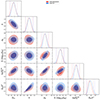 |
Fig. 7. 68% and 95% parameter constraint contours from one example of the test dataset using FullB-SeResNet and Full-FCN. The diagonal plots are the marginalised parameter constraints, and the dashed black lines stand for the true values reported in Table 6. The vertical dashed red and blue lines represent the 1σ for the marginals using FullB-SeResNet and Full-FCN, respectively. We derived these posterior distributions using GetDist (Lewis 2019). |
Parameters in the 95% intervals taken from the parameter constraint contours from one example of the MG simulations test set predicted by the FullB-SeResnet18 and FullB-FCN.
6. Summary and discussion
We considered a wide range of MG simulations for which we varied the cosmological parameters. They encompassed cosmologies with large deviations from the standard GR to parameters closest to those that mimic the dynamics of a Universe based on GR. The overdensity field of each snapshot was computed using the CIC mass assignment, and subsequently, we obtained its power spectrum. To constrain the main set of cosmological parameters, we introduced a novel architecture of a BNN and designed several experiments to test its ability to predict MG cosmologies. The experiments consist of building two Bayesian networks based on stochastic layers located at either the top or at all levels of the architecture. This approach was motivated by the question of whether BNNs provide a better accuracy and robustness performance when we work with full or partial network configurations. Starting from the 3D overdensity field, we found that although the FullB predicts the cosmological parameters slightly better than the BLL, the latter is accurate enough to retrieve cosmological information from the density field, especially for Ωm and σ8. Similarly, we tested BNNs using the two-point statistics described by the power spectrum for reasonable scales limited by the Nyquist frequency. The results of this experiment show that the information learned by the networks can predict the parameters with an accuracy similar to the 3D field. Both configurations of the BNN architectures fall short of capturing both the Hubble parameter and the MG effects. This underscores the necessity of improving the training dataset in terms of resolution and scale for the 3D density setup. Despite the slight constraints for some cosmological parameters, the method can be relevant in applications where it is combined with classical inference methods (Hortúa et al. 2020a). The multiplicative normalising flows technique in BNNs employed in this paper has proved to yield good predictions and accurate uncertainty estimates through the ability to transform the approximate posterior into a more expressive distribution consistent with the data complexity. This is a significant improvement compared to standard VI, where the posterior is restricted to a Gaussian configuration. Nevertheless, the effect of assuming a Gaussian prior distribution of the weights under this approach is still unknown (Fortuin et al. 2021). In future work, we will explore multiplicative normalising flows with different prior distributions over the weights and analyse how the prior influences the uncertainty calibration and performance.
The finding that the MG parameter is poorly predicted when the information provided by the density field is used demonstrates, on the one hand, the effectiveness of the chameleon screening mechanism in mimicking the ΛCDM model, and on the other hand, the need for further analysis with other datasets that are more sensitive to the effects of MG. We considered parameters that produce the same effect, that is, that are degenerate. Therefore, it is not straightforward to attribute a single characteristic of the overdensity field exclusively to a single parameter, as in the case of fR0 and σ8. The proposed architectures are sufficiently general from a statistical standpoint to estimate posterior distributions. However, this study has revealed that the available information is inadequate to predict all parameters solely from a single source. This underscores the significance of resolving degeneracies between cosmological parameters by incorporating supplementary data or diverse features present in the cosmological simulations. This approach enables the BNNs to gain a richer learning phase and parse out the signals of each cosmology. This task will be the focus of a forthcoming paper, where we plan to evaluate the BNN robustness using simulations of higher resolution and more intricate datasets in redshift space, incorporating velocity information alongside particle positions.
In Table 7, we also presented a comparison of the relative errors for the two best-estimated parameters using CNN and N-body simulations from the literature. We observed significant discrepancies in the relative errors of σ8 and Ωm, approximately 90% when Bayesian inference is not employed (see Ravanbakhsh et al. 2017; Pan et al. 2020). This outcome arises from using solely ΛCDM simulations in both training and test datasets, in contrast to our estimates, which encompass an additional parameter accounting for MG and include a calibration procedure of the uncertainties. Furthermore, when comparing the performance of BLL architectures on MG and ΛCDM simulations, such as QUIJOTE (see e.g. Hortúa et al. 2023), we find a deviation of the relative errors close to 30% when MG effects are not considered. This result clarifies that when using FullB-SeResNet18, the error bars for Ωm are 1.3 times larger and are larger by 2.1 times for σ8 in comparison to FlipoutBNN. In the context of BNNs, when separately considering the two cosmological models MG and ΛCDM, we assessed the performance in terms of the MSE metric by comparing it to the results presented by Hortúa et al. (2023), who employed a similar architecture. Specifically, using FullBs in both cosmological models, we observed an improvement by a factor 13 in the MSE of the MG predictions over the ΛCDM ones. The r2 metric was used to compare the confidence range of the individual parameters. In terms of this metric, we report that σ8 deviates more (r2 = 0.95 in MG and r2 = 0.99 in ΛCDM), which accounts for 4.2% of the expected uncertainty. The marginal difference in the coefficient of determination for predicting Ωm is only 0.01 when comparing the results of the model trained with MG against the model trained with ΛCDM. In both cases, it is noteworthy that a high r2 value does not necessarily confer complete certainty regarding individual parameter estimates, particularly when the parameter degeneracy is taken into account. Furthermore, one interesting possibility to refine the constraints on f(R) gravity is given by training a specialised network that clearly distinguishes between ΛCDM and f(R), offering the potential to detect a non-zero fR0. Further investigations, including high-resolution simulations as well as extensions beyond ΛCDM, promise to further enhance the capabilities of the BNNs approach. The BNNs prove valuable in constructing mock catalogues for galaxy surveys, excelling in tasks such as object classification and feature extraction. The synergy of BNNs with galaxy painting techniques further strengthens the ability to capture complex patterns in the data, offering valuable insights into large-scale studies. The BNN model we developed can be readily adapted for the analysis of observational data. However, this modification requires a more substantial effort in appropriately processing the inputs to align with the noise level inherent in dedicated galaxy surveys. Addressing challenges such as bias, sample tracers, peculiar motions, and the systematic from galaxy surveys becomes imperative in this context. They might nonetheless be implemented in Bayesian inference algorithms of the large-scale structure (such as, e.g., Kitaura et al. 2021). Together with this paper, we make the scripts available, which can be accessed at the public github repository of the project12.
Relative error comparison of the different CNN approaches for MG and ΛCDM simulations.
7. Conclusions
One of the intriguing possibilities to explain the observed accelerated expansion of the Universe is the modification of general relativity on large scales. Matter distribution analysis via N-body simulations offers a perfect scenario to track departures from standard gravity. Among different parametrisations, f(R) has emerged as an interesting model because it can reproduce the standard model predictions accurately. In this paper, we analysed the possibility of using Bayesian deep-learning methods for constraining cosmological parameters from MG simulations. Below, we summarise the main takeaways from this study.
-
BNNs can predict cosmological parameters with a higher accuracy, especially for Ωm and σ8 from the overdensity field. However, based on the assumption of simulating boxes with 256 h−1 Mpc to acquire MG effects on large scales, BNNs were unable to effectively extract MG patterns from the overdensity field to yield an accurate f(R) parameter estimation. However, when comparing the parameter estimation with ΛCDM-only simulations, the uncertainties of σ8 are significantly underpredicted when possible MG effects are not taken into account. In addition, special attention should be paid to parameter degeneracies that may be present not only in two-point statistics, but in more features of the density field. We conclude that higher resolution and further intricate datasets in redshift space, incorporating velocity information alongside particle positions, can be approaches that should be addressed to improve the network predictions.
-
It is observed that cosmological parameters can be recovered directly from the simulations using convolution-based models with the potential of extracting patterns without specifying any N-point statistics beforehand. This is supported by the fact that networks trained with overdensity fields and power spectra yielded decent predictions, but with distinctive correlations among the parameters. 3D convolutions extracted supplementary information beyond the linear regime, which allowed them to constrain the parameter estimation tightly.
-
We generalised the multiplicative normalising flows for BNNs to the 3D convolutional level, which allowed us to work with fully transformed stochastic neural networks. As a proof of concept, we ran several experiments to verify that this approach not only achieved the performance reached by the deterministic models, but also yielded well-calibrated uncertainty estimates.
-
We probed the impact of the parameter estimation based on the Bayesian last layer (BLL) and fully Bayesian approaches. The results showed that fullBs provide slightly higher-quality predictions along with accurate uncertainty estimates. Nevertheless, this improvement is not significant enough to prefer this approach to the BLL, where the latter has the advantage of being relatively model agnostic, easily scalable, and is twice as fast in inference time.
-
Several experiments have reported that normalising flows added at the output layers as well to avoid bottlenecks by the simple multivariate distribution do not improve the model performance significantly. We therefore decided to work with the simple distribution as output for the network.
The code can be found at https://github.com/HAWinther/MG-PICOLA-PUBLIC
Acknowledgments
This paper is based on work supported by the Google Cloud Research Credits program with the award GCP19980904. H.H. acknowledges support from créditos educación de doctorados nacionales y en el exterior-Colciencias and the grant provided by the Google Cloud Research Credits program. J.E.G.F. is supported by the Spanish Ministry of Universities, through a María Zambrano grant (program 2021–2023) at Universidad de La Laguna with reference UP2021-022, funded within the European Union-Next Generation EU. F.S.K. and J.E.G.F. acknowledge the IAC facilities and the Spanish Ministry of Science and Innovation (MICINMINECO) under project PID2020-120612GB-I00. We also thank the personnel of the Servicios Informáticos Comunes (SIC) of the IAC.
References
- Abadi, M., Agarwal, A., Barham, P., et al. 2016, arXiv e-prints [arXiv:1603.04467] [Google Scholar]
- Abdar, M., Pourpanah, F., Hussain, S., et al. 2021, Inf. Fusion, 76, 243 [CrossRef] [Google Scholar]
- Alves de Oliveira, R., Li, Y., Villaescusa-Navarro, F., Ho, S., & Spergel, D. N. 2020, ArXiv e-prints [arXiv:2012.00240] [Google Scholar]
- Beaumont, M. A. 2010, Annu. Rev. Ecol. Evol. Syst., 41, 379 [Google Scholar]
- Berti, E., Barausse, E., Cardoso, V., et al. 2015, Class. Quant. Grav., 32, 243001 [NASA ADS] [CrossRef] [Google Scholar]
- Blundell, C., Cornebise, J., Kavukcuoglu, K., & Wierstra, D. 2015, Proceedings of the 32nd International Conference on International Conference on Machine Learning – Volume 37, ICML’15 (JMLR), 1613 [Google Scholar]
- Bos, E. G. P., van de Weygaert, R., Dolag, K., & Pettorino, V. 2012, MNRAS, 426, 440 [NASA ADS] [CrossRef] [Google Scholar]
- Brown, Z., Mishtaku, G., & Demina, R. 2022, A&A, 667, A129 [NASA ADS] [CrossRef] [EDP Sciences] [Google Scholar]
- Cai, Y.-C., Padilla, N., & Li, B. 2015, MNRAS, 451, 1036 [NASA ADS] [CrossRef] [Google Scholar]
- Charnock, T., Perreault-Levasseur, L., & Lanusse, F. 2022, Bayesian Neural Networks (World Scientific), 663 [Google Scholar]
- Contarini, S., Marulli, F., Moscardini, L., et al. 2021, MNRAS, 504, 5021 [NASA ADS] [CrossRef] [Google Scholar]
- Crocce, M., Pueblas, S., & Scoccimarro, R. 2006, MNRAS, 373, 369 [NASA ADS] [CrossRef] [Google Scholar]
- Crocce, M., Pueblas, S., & Scoccimarro, R. 2012, Astrophysics Source Code Library [record ascl:1201.005] [Google Scholar]
- Csilléry, K., Blum, M. G., Gaggiotti, O. E., & François, O. 2010, Trends Ecol. Evol., 25, 410 [CrossRef] [Google Scholar]
- De Felice, A., & Tsujikawa, S. 2010, Liv. Rev. Relat., 13, 3 [NASA ADS] [CrossRef] [Google Scholar]
- Deng, W., Zhang, X., Liang, F., & Lin, G. 2019, Bayesian Deep Learning via Stochastic Gradient MCMC with a Stochastic Approximation Adaptation, https://openreview.net/forum?id=S1grRoR9tQ [Google Scholar]
- Denker, J. S., & LeCun, Y. 1990, Proceedings of the 3rd International Conference on Neural Information Processing Systems, NIPS’90 (San Francisco: Morgan Kaufmann Publishers Inc.), 853 [Google Scholar]
- Dinh, L., Sohl-Dickstein, J., & Bengio, S. 2017, International Conference on Learning Representations, https://openreview.net/forum?id=HkpbnH9lx [Google Scholar]
- Dong, F., Park, C., Hong, S. E., et al. 2023, ApJ, 953, 98 [NASA ADS] [CrossRef] [Google Scholar]
- Dvorkin, C., Mishra-Sharma, S., Nord, B., et al. 2022, ArXiv e-prints [arXiv:2203.08056] [Google Scholar]
- Fang, W., Li, B., & Zhao, G.-B. 2017, Phys. Rev. Lett., 118, 181301 [NASA ADS] [CrossRef] [Google Scholar]
- Fiedler, F., & Lucia, S. 2023, IEEE Access, 11, 123149 [NASA ADS] [CrossRef] [Google Scholar]
- Fluri, J., Kacprzak, T., Sgier, R., Refregier, A., & Amara, A. 2018, JCAP, 2018, 051 [CrossRef] [Google Scholar]
- Fortuin, V., Garriga-Alonso, A., Ober, S. W., et al. 2021, ArXiv e-prints [arXiv:2102.06571] [Google Scholar]
- Gal, Y. 2016, PhD Thesis, University of Cambridge, UK [Google Scholar]
- Gal, Y., & Ghahramani, Z. 2016, in Proceedings of the 33rd International Conference on Machine Learning, eds. M. F. Balcan, & K. Q. Weinberger (New York: PMLR), Proc. Mach. Learn. Res., 48, 1050 [Google Scholar]
- García-Farieta, J. E., Marulli, F., Veropalumbo, A., et al. 2019, MNRAS, 488, 1987 [Google Scholar]
- García-Farieta, J. E., Marulli, F., Moscardini, L., Veropalumbo, A., & Casas-Miranda, R. A. 2020, MNRAS, 494, 1658 [CrossRef] [Google Scholar]
- García-Farieta, J. E., Hellwing, W. A., Gupta, S., & Bilicki, M. 2021, Phys. Rev. D, 103, 103524 [CrossRef] [Google Scholar]
- Graves, A. 2011, Practical Variational Inference for Neural Networks (Curran Associates, Inc.), 24 [Google Scholar]
- Gunapati, G., Jain, A., Srijith, P. K., & Desai, S. 2022, PASA, 39, e001 [NASA ADS] [CrossRef] [Google Scholar]
- Guo, C., Pleiss, G., Sun, Y., & Weinberger, K. Q. 2017, Proceedings of the 34th International Conference on Machine Learning – Volume 70, ICML’17 (JMLR), 1321 [Google Scholar]
- Gupta, S., Hellwing, W. A., Bilicki, M., & García-Farieta, J. E. 2022, Phys. Rev. D, 105, 043538 [NASA ADS] [CrossRef] [Google Scholar]
- Hagstotz, S., Costanzi, M., Baldi, M., & Weller, J. 2019, MNRAS, 486, 3927 [Google Scholar]
- Hahn, C., Eickenberg, M., Ho, S., et al. 2022, ArXiv e-prints [arXiv:2211.00723] [Google Scholar]
- Hamaus, N., Pisani, A., Sutter, P. M., et al. 2016, Phys. Rev. Lett., 117, 091302 [NASA ADS] [CrossRef] [Google Scholar]
- Harnois-Déraps, J., Martinet, N., Castro, T., et al. 2021, MNRAS, 506, 1623 [CrossRef] [Google Scholar]
- Henning, C., D’Angelo, F., & Grewe, B. F. 2021, ArXiv e-prints [arXiv:2107.12248] [Google Scholar]
- Hernández-Aguayo, C., Hou, J., Li, B., Baugh, C. M., & Sánchez, A. G. 2019, MNRAS, 485, 2194 [CrossRef] [Google Scholar]
- Hernández-Aguayo, C., Ruan, C.-Z., Li, B., et al. 2022, JCAP, 2022, 048 [CrossRef] [Google Scholar]
- Hikage, C., Schmalzing, J., Buchert, T., et al. 2003, PASJ, 55, 911 [NASA ADS] [Google Scholar]
- Hockney, R. W., & Eastwood, J. W. 1981, Computer Simulation Using Particles (New York: McGraw-Hill) [Google Scholar]
- Hortua, H. J. 2021, ArXiv e-prints [arXiv:2112.11865] [Google Scholar]
- Hortúa, H. J., Volpi, R., Marinelli, D., & Malagò, L. 2020a, Phys. Rev. D, 102, 103509 [CrossRef] [Google Scholar]
- Hortúa, H. J., Malagò, L., & Volpi, R. 2020b, Mach. Learn.: Sci. Technol., 1, 035014 [CrossRef] [Google Scholar]
- Hortúa, H. J., García, L., & Castaneda, L. 2023, Front. Astron. Space Sci., 10, 1139120 [CrossRef] [Google Scholar]
- Howlett, C., Manera, M., & Percival, W. J. 2015, Astron. Comput., 12, 109 [NASA ADS] [CrossRef] [Google Scholar]
- Hu, W., & Sawicki, I. 2007, Phys. Rev. D, 76, 064004 [CrossRef] [Google Scholar]
- Hu, J., Shen, L., Albanie, S., Sun, G., & Wu, E. 2017, ArXiv e-prints [arXiv:1709.01507] [Google Scholar]
- Ivarsen, M. F., Bull, P., Llinares, C., & Mota, D. 2016, A&A, 595, A40 [NASA ADS] [CrossRef] [EDP Sciences] [Google Scholar]
- Jennings, E., Baugh, C. M., Li, B., Zhao, G.-B., & Koyama, K. 2012, MNRAS, 425, 2128 [NASA ADS] [CrossRef] [Google Scholar]
- Johnson, A., Blake, C., Dossett, J., et al. 2016, MNRAS, 458, 2725 [NASA ADS] [CrossRef] [Google Scholar]
- Kacprzak, T., Kirk, D., Friedrich, O., et al. 2016, MNRAS, 463, 3653 [Google Scholar]
- Kilbinger, M. 2015, Rep. Progr. Phys., 78, 086901 [Google Scholar]
- Kingma, D. P., & Ba, J. 2014, ArXiv e-prints [arXiv:1412.6980] [Google Scholar]
- Kitaura, F.-S., Ata, M., Rodríguez-Torres, S. A., et al. 2021, MNRAS, 502, 3456 [NASA ADS] [CrossRef] [Google Scholar]
- Koda, J., Blake, C., Beutler, F., Kazin, E., & Marin, F. 2016, MNRAS, 459, 2118 [NASA ADS] [CrossRef] [Google Scholar]
- Kodi Ramanah, D., Charnock, T., Villaescusa-Navarro, F., & Wandelt, B. D. 2020, MNRAS, 495, 4227 [NASA ADS] [CrossRef] [Google Scholar]
- Kostić, A., Nguyen, N.-M., Schmidt, F., & Reinecke, M. 2023, JCAP, 2023, 063 [Google Scholar]
- Kratochvil, J. M., Lim, E. A., Wang, S., et al. 2012, Phys. Rev. D, 85, 103513 [Google Scholar]
- Lakshminarayanan, B., Pritzel, A., & Blundell, C. 2017, Proceedings of the 31st International Conference on Neural Information Processing Systems, NIPS’17 (Red Hook: Curran Associates Inc.), 6405 [Google Scholar]
- Laszlo, I., & Bean, R. 2008, Phys. Rev. D, 77, 024048 [CrossRef] [Google Scholar]
- Lavaux, G., & Wandelt, B. D. 2010, MNRAS, 403, 1392 [NASA ADS] [CrossRef] [Google Scholar]
- Laves, M. H., Ihler, S., Fast, J. F., Kahrs, L. A., & Ortmaier, T. 2020, Medical Imaging with Deep Learning, https://openreview.net/forum?id=CecZ_0t79q [Google Scholar]
- Lazanu, A. 2021, JCAP, 2021, 039 [CrossRef] [Google Scholar]
- Lemos, P., Cranmer, M., Abidi, M., et al. 2023a, Mach. Learn.: Sci. Technol., 4, 01LT01 [NASA ADS] [CrossRef] [Google Scholar]
- Lemos, P., Parker, L. H., Hahn, C., et al. 2023b, Machine Learning for Astrophysics, Workshop at the Fortieth International Conference on Machine Learning (ICML 2023), July 29th, Hawaii, USA, online at https://ml4astro.github.io/icml2023/, 18 [Google Scholar]
- Lewis, A. 2019, ArXiv e-prints [arXiv:1910.13970] [Google Scholar]
- Li, B., Zhao, G.-B., Teyssier, R., & Koyama, K. 2012, JCAP, 2012, 051 [CrossRef] [Google Scholar]
- Li, X.-D., Park, C., Sabiu, C. G., & Kim, J. 2015, MNRAS, 450, 807 [NASA ADS] [CrossRef] [Google Scholar]
- Louizos, C., & Welling, M. 2017, Proceedings of the 34th International Conference on Machine Learning – Volume 70, ICML’17 (JMLR), 2218 [Google Scholar]
- Luo, X., Wu, Z., Li, M., et al. 2019, ApJ, 887, 125 [NASA ADS] [CrossRef] [Google Scholar]
- Lyall, S., Blake, C., Turner, R., Ruggeri, R., & Winther, H. 2023, MNRAS, 518, 5929 [Google Scholar]
- Mancarella, M., Kennedy, J., Bose, B., & Lombriser, L. 2022, Phys. Rev. D, 105, 023531 [NASA ADS] [CrossRef] [Google Scholar]
- McCarthy, I. G., Salcido, J., Schaye, J., et al. 2023, MNRAS, 526, 5494 [NASA ADS] [CrossRef] [Google Scholar]
- Merten, J., Giocoli, C., Baldi, M., et al. 2019, MNRAS, 487, 104 [Google Scholar]
- Moresco, M., Amati, L., Amendola, L., et al. 2022, Liv. Rev. Relat., 25, 6 [NASA ADS] [Google Scholar]
- Nguyen, N.-M., Huterer, D., & Wen, Y. 2023, Phys. Rev. Lett., 131, 111001 [CrossRef] [Google Scholar]
- Nojiri, S., Odintsov, S. D., & Oikonomou, V. K. 2017, Phys. Rep., 692, 1 [NASA ADS] [CrossRef] [Google Scholar]
- Odintsov, S. D., Oikonomou, V. K., Giannakoudi, I., Fronimos, F. P., & Lymperiadou, E. C. 2023, Symmetry, 15, 1701 [NASA ADS] [CrossRef] [Google Scholar]
- Paillas, E., Cai, Y.-C., Padilla, N., & Sánchez, A. G. 2021, MNRAS, 505, 5731 [NASA ADS] [CrossRef] [Google Scholar]
- Pan, S., Liu, M., Forero-Romero, J., et al. 2020, Sci. China Phys. Mech. Astron., 63, 110412 [NASA ADS] [CrossRef] [Google Scholar]
- Park, C., & Kim, Y.-R. 2010, ApJ, 715, L185 [NASA ADS] [CrossRef] [Google Scholar]
- Peebles, P. J. E. 2001, in Historical Development of Modern Cosmology, eds. V. J. Martínez, V. Trimble, & M. J. Pons-Bordería, ASP Conf. Ser., 252, 201 [NASA ADS] [Google Scholar]
- Peel, A., Lin, C.-A., Lanusse, F., et al. 2017, A&A, 599, A79 [NASA ADS] [CrossRef] [EDP Sciences] [Google Scholar]
- Peel, A., Lalande, F., Starck, J.-L., et al. 2019, Phys. Rev. D, 100, 023508 [Google Scholar]
- Perico, E. L. D., Voivodic, R., Lima, M., & Mota, D. F. 2019, A&A, 632, A52 [NASA ADS] [CrossRef] [EDP Sciences] [Google Scholar]
- Philcox, O. H. E., Slepian, Z., Hou, J., et al. 2022, MNRAS, 509, 2457 [Google Scholar]
- Planck Collaboration VI. 2020, A&A, 641, A6 [NASA ADS] [CrossRef] [EDP Sciences] [Google Scholar]
- Puchwein, E., Baldi, M., & Springel, V. 2013, MNRAS, 436, 348 [NASA ADS] [CrossRef] [Google Scholar]
- Ravanbakhsh, S., Oliva, J., Fromenteau, S., et al. 2017, ArXiv e-prints [arXiv:1711.02033] [Google Scholar]
- Sønderby, C. K., Raiko, T., Maaløe, L., Sønderby, S. K., & Winther, O. 2016, Proceedings of the 30th International Conference on Neural Information Processing Systems, NIPS’16 (Red Hook: Curran Associates Inc.), 3745 [Google Scholar]
- Song, Y.-S., Hu, W., & Sawicki, I. 2007, Phys. Rev. D, 75, 044004 [CrossRef] [Google Scholar]
- Sunnåker, M., Busetto, A. G., Numminen, E., et al. 2013, PLOS Comput. Biol., 9, 1 [Google Scholar]
- Takada, M., & Jain, B. 2003, MNRAS, 340, 580 [NASA ADS] [CrossRef] [Google Scholar]
- Tamosiunas, A., Winther, H. A., Koyama, K., et al. 2021, MNRAS, 506, 3049 [NASA ADS] [CrossRef] [Google Scholar]
- Tassev, S., Zaldarriaga, M., & Eisenstein, D. J. 2013, JCAP, 2013, 036 [Google Scholar]
- Thomas, O., Dutta, R., Corander, J., Kaski, S., & Gutmann, M. U. 2016, ArXiv e-prints [arXiv:1611.10242] [Google Scholar]
- Touati, A., Satija, H., Romoff, J., Pineau, J., & Vincent, P. 2018, ArXiv e-prints [arXiv:1806.02315] [Google Scholar]
- Tsujikawa, S. 2008, Phys. Rev. D, 77, 023507 [NASA ADS] [CrossRef] [Google Scholar]
- Tsujikawa, S., Uddin, K., Mizuno, S., Tavakol, R., & Yokoyama, J. 2008, Phys. Rev. D, 77, 103009 [NASA ADS] [CrossRef] [Google Scholar]
- Van Waerbeke, L., Mellier, Y., Radovich, M., et al. 2001, A&A, 374, 757 [NASA ADS] [CrossRef] [EDP Sciences] [Google Scholar]
- Veropalumbo, A., Binetti, A., Branchini, E., et al. 2022, JCAP, 2022, 033 [CrossRef] [Google Scholar]
- Villaescusa-Navarro, F., Hahn, C., Massara, E., et al. 2020, ApJS, 250, 2 [CrossRef] [Google Scholar]
- Voivodic, R., Lima, M., Llinares, C., & Mota, D. F. 2017, Phys. Rev. D, 95, 024018 [CrossRef] [Google Scholar]
- Watson, J., Andreas Lin, J., Klink, P., Pajarinen, J., & Peters, J. 2021, in Proceedings of The 24th International Conference on Artificial Intelligence and Statistics, eds. A. Banerjee, & K. Fukumizu (PMLR), Proc. Mach. Learn. Res., 130, 1198 [Google Scholar]
- Weinberg, D. H., Mortonson, M. J., Eisenstein, D. J., et al. 2013, Phys. Rep., 530, 87 [Google Scholar]
- Wen, Y., Vicol, P., Ba, J., Tran, D., & Grosse, R. 2018, International Conference on Learning Representations, https://openreview.net/forum?id=rJNpifWAb [Google Scholar]
- Winther, H. A., Koyama, K., Manera, M., Wright, B. S., & Zhao, G.-B. 2017, JCAP, 2017, 006 [CrossRef] [Google Scholar]
- Zhang, Z., Gu, G., Wang, X., et al. 2019, ApJ, 878, 137 [NASA ADS] [CrossRef] [Google Scholar]
- Zhang, H., Samushia, L., Brooks, D., et al. 2022, MNRAS, 515, 6133 [NASA ADS] [CrossRef] [Google Scholar]
All Tables
Configuration of the (Se)-ResNet backbone used for all experiments presented in this paper.
Configuration of the fully connected neural network used for constraining the parameters from the power spectrum.
Parameters in the 95% intervals taken from the parameter constraint contours from one example of the MG simulations test set predicted by the FullB-SeResnet18 and FullB-FCN.
Relative error comparison of the different CNN approaches for MG and ΛCDM simulations.
All Figures
|
Fig. 1. Multidimensional parameter space variations. Each line represents the parameter values of a data point. The four parameters Ωm, h, σ8, and 0.1log10|fR0| are visualised along separate axes. |
| In the text | |
|
Fig. 2. Projected overdensity field at redshift z = 0 derived from an arbitrarily chosen simulation within the ensemble of 2500 MG simulations. The normalised density field was calculated using a CIC mass-assignment scheme. |
| In the text | |
|
Fig. 3. Projected density field of dark matter in a region of 256 × 256 × 20 (h−1 Mpc)3 from 100 out of 2500 arbitrarily chosen simulations of MG. The snapshots are taken at z = 0, and the legend displays the set of cosmological parameters of {Ωm, h, σ8, fR0}. The cuts in the density field highlight the broad coverage of the parameter space of the MG simulations. Different features can be observed by naked eye, such as variations in the filament structure of the cosmic web. |
| In the text | |
|
Fig. 4. Matter power spectrum at z = 0 of the MG simulation suit. The variations in the spectrum correspond to changes in each of the four parameters that were varied, Ωm, h, σ8 and |0.1 log fR0|. The corresponding range of each of parameter is shown in the label. |
| In the text | |
|
Fig. 5. Resblock schema depending on the architecture used. Top: resblock when SeResNet18 is employed. The dashed orange rectangle shows the skip SE-connection schema used in the SeResNet18 resblock. Bottom: resblock when ResNet is employed. |
| In the text | |
|
Fig. 6. True vs. predicted values provided by the FullB model for Ωm, σ8, and some derivative parameters. The points are the mean of the predicted distributions, and the error bars stand for the heteroscedastic uncertainty associated with the epistemic and aleatoric uncertainty at 1σ. |
| In the text | |
|
Fig. 7. 68% and 95% parameter constraint contours from one example of the test dataset using FullB-SeResNet and Full-FCN. The diagonal plots are the marginalised parameter constraints, and the dashed black lines stand for the true values reported in Table 6. The vertical dashed red and blue lines represent the 1σ for the marginals using FullB-SeResNet and Full-FCN, respectively. We derived these posterior distributions using GetDist (Lewis 2019). |
| In the text | |
Current usage metrics show cumulative count of Article Views (full-text article views including HTML views, PDF and ePub downloads, according to the available data) and Abstracts Views on Vision4Press platform.
Data correspond to usage on the plateform after 2015. The current usage metrics is available 48-96 hours after online publication and is updated daily on week days.
Initial download of the metrics may take a while.