| Issue |
A&A
Volume 697, May 2025
|
|
|---|---|---|
| Article Number | A66 | |
| Number of page(s) | 28 | |
| Section | Extragalactic astronomy | |
| DOI | https://doi.org/10.1051/0004-6361/202347707 | |
| Published online | 07 May 2025 | |
Probing circular polarization and magnetic field structure in active galactic nuclei
1
Max-Planck-Institut für Radioastronomie, Auf dem Hügel 69, D-53121 Bonn, Germany
2
Theoretical Division, Los Alamos National Laboratory, Los Alamos, NM 87545, USA
3
National Radio Astronomy Observatory, P.O. Box O Socorro, NM 87801, USA
4
Instituto de Astrofísica de Andalucía, Gta. de la Astronomia, s/n, Genil, 18008 Granada, Spain
⋆ Corresponding author: jah@lanl.gov, jkramer@mpifr.de
Received:
11
August
2023
Accepted:
9
March
2025
Context. The composition and magnetic field morphology of relativistic jets can be studied using circular polarization (CP) measurement. Recent three-dimensional relativistic magnetohydrodynamic (3D RMHD) simulations coupled with radiative transfer (RT) calculations make strong predictions about the level (and morphology) of the jet’s CP emission. These simulations show that the sign of CP and the electric vector position angle (EVPA) are both sensitive to the jet’s magnetic field morphology within the radio core.
Aims. We probe this theory by exploring whether the jet’s radio core EVPA orientation is consistent with the observed sign of the core CP in deep full-track polarimetric observations. Based on a selection of sources from earlier MOJAVE observations, we aim to probe the nature of linear polarization (LP) and CP in the innermost regions of jets from a small sample of nine blazars. This sample includes sources that have exhibited: (i) positive CP; (ii) negative CP; or (iii) positive and negative CP simultaneously in the radio core region. By coupling deep polarimetric observations of a carefully selected sample of blazars with state-of-the-art RMHD and RT calculations, we hope to gain a deeper understanding of the physics of blazar jets.
Methods. Nine blazar sources were observed using the VLBA at both 15 GHz and 23 GHz. Standard AIPS calibration was applied. Our self-calibration relies on a physically based model applied in DoG-HiT resulting in more accurate gains. To improve the imaging quality, we used specialized algorithms, such as DoG-HiT, which excel in their handling of compact emission.
Results. We observe robust, relatively high degrees of fractional circular polarization |m̄c| ≃ (0.32 ± 0.2)% at 15 GHz and |m̄c| ≃ (0.59 ± 0.56)% at 23 GHz. We observe consistent polarized structure and EVPA orientation over time when comparing our analysis with archival MOJAVE data. Theoretical predictions indicate a clearly favored toroidal magnetic field orientation within the extended jet emission of the reconstructed signal of the blazar 0149+218. At 23 GHz, the jet structures of 1127–145 and 0528+134 (even at super-resolution) exhibit characteristics that are aligned with a helical or poloidal magnetic nature. Changes in the CP sign as the frequency transitions from 15 GHz to 23 GHz suggest the influence of optical depth effects.
Key words: magnetic fields / polarization / instrumentation: interferometers / methods: observational / BL Lacertae objects: general / galaxies: jets
© The Authors 2025
 Open Access article, published by EDP Sciences, under the terms of the Creative Commons Attribution License (https://creativecommons.org/licenses/by/4.0), which permits unrestricted use, distribution, and reproduction in any medium, provided the original work is properly cited.
This article is published in open access under the Subscribe to Open model.
Open access funding provided by Max Planck Society.
1. Introduction
Supermassive black holes (SMBH) in the centers of galaxies are some of the most prominent emitters of high-energy radiation in the universe. Such objects, known as active galactic nuclei (AGN), are driven by the accretion of matter onto their central SMBH. Their emission spans across the entire electromagnetic spectrum, from radio to gamma ray energies, although only about 10% are referred to as “radio-loud” AGN (Kellermann et al. 1989).
When matter is accreted onto a BH, outflows from highly collimated plasma, called jets, form along its polar axis. Such jets are mostly visible (and studied) at radio wavelengths, identified as non-thermal synchrotron radiation emitted by charged particles spiraling around magnetic field lines at relativistic speeds. Synchrotron radiation has the potential to be significantly linearly polarized, reaching up to 75% in the presence of a uniform magnetic field (Pacholczyk 1970; Troja et al. 2017). Linear polarization (LP) observations can provide valuable information about the orientation and morphology of the magnetic field structure within the synchrotron-emitting source. In addition, LP observations provide valuable information about the distribution of thermal electrons and the geometry of the magnetic field in the immediate vicinity of the AGN.
Polarization in AGN was first discovered in the optical regime (e.g., Heeschen 1973) and soon after at millimeter wavelengths (e.g., Kinman & Conklin 1971; Rudnick et al. 1978). In the late 1960s, very long baseline interferometry (VLBI) was applied for high angular resolution studies. The first polarized VLBI images were published in the mid-1980s (Cotton et al. 1984; Roberts & Wardle 1986). To this day, VLBI imaging allows us to observe, resolve, and study polarized radiation emitted from both in the innermost regions of AGN (e.g., Event Horizon Telescope Collaboration 2021; Issaoun et al. 2022; Jorstad et al. 2023) and their relativistic jets on the kilo-parsec (kpc) scale (e.g., MacDonald et al. 2017; Hodge et al. 2018; Zobnina et al. 2023; Pushkarev et al. 2023).
Commonly, LP is expressed in terms of the electric vector position angle (EVPA) in a VLBI image or as the fractional polarization in some area of the jet with respect to the total intensity peak. Since the EVPA is predicted to be perpendicular to the local magnetic field, polarized images help us understand the magnetic field geometry in the source. For example, extended jets up to kilo-parsecs tend to show EVPAs perpendicular to the direction of jet motion, indicating a poloidal or helical magnetic field. In turn, if the EVPAs are oriented parallel to the jet, the magnetic field is toroidal, which is a characteristic of shock compression (Contopoulos et al. 2015). A bi-modal EVPA pattern with a difference between the jet spine and sheath is indicated in theoretical models of 3D RMHD jet simulations (Kramer & MacDonald 2021).
Only the smallest fraction of the observed emission is circularly polarized (CP, Stokes V); in fact, the CP fraction only rarely even reaches 1% and usually falls well below that (Wardle 2021). Nonetheless, the use of Very Long Baseline Array (VLBA) observations has enabled the analysis of circular polarization in extragalactic jets with exceptional precision, operating at sub-milliarcsecond resolution. Pioneering studies by Wardle et al. (1998) and Homan & Wardle (1999) revealed circular polarization in the central regions of four robust AGN jets, exhibiting local fractional levels ranging from 0.3% to 1% of Stokes I when observed with the VLBA.
Circular polarization has subsequently been identified in other AGN jets using different instruments, as documented by Rayner et al. (2000), Homan & Lister (2006), and Vitrishchak et al. (2008). The observed CP is thought to originate either from intrinsic synchrotron processes, or from LP converted to CP by Faraday rotation (e.g., MacDonald 2017). In AGN jets, CP can serve as a powerful tool for probing the particle composition and magnetic field morphology both at large scales and near the launching site. The first detection of CP in AGN jets was reported in the late 1990s in VLBI observations of the quasar 3C 279 (Wardle et al. 1998). The strongest signal detected in an AGN jet is observed in 3C 84 by Homan & Wardle (2004).
In this work, we present the first comparison of CP maps obtained from VLBI observations with the VLBA and synthetic polarized emission maps produced with the PLUTO Code (Kramer & MacDonald 2021). This paper is structured as follows: In Sects. 2 and 3, the methodology is outlined, including details of the 15 GHz and 23 GHz VLBI observations and the calibration procedures. This includes polarization calibration with particular emphasis on enhancing Stokes V and rectifying compact polarized emission signals using the DoG-HiT imaging software. Our results are presented in Sect. 4, where we show polarized intensity maps and describe the polarized structures of the nine observed blazar sources. A super-resolution perspective on 0528+134 is also provided. In Sect. 5, the results are thoroughly dissected and analyzed. This includes a view on archival MOJAVE data. Finally, Sect. 6 summarizes the final conclusions drawn from the resulting maps in the context of physical concepts.
2. Methodology and observations
2.1. Methodology
Over 400 AGN jets have been observed as a part of the MOJAVE monitoring program with the VLBA from 1996 to 20161. From this long-term effort, the following conclusions could be drawn:
-
fractional polarization in jets increases with separation from the total intensity peak and towards the jet edges of the VLBI core;
-
40% of the VLBI cores have a preferred EVPA direction across multiple epochs;
-
EVPAs in jets of BL Lac objects, as well as in their radio cores, are more stable than those in quasars. Additionally, the EVPAs tend to be aligned with the initial jet direction (Pushkarev et al. 2017).
Within the MOJAVE program, it was possible to observe CP at very faint levels within some jets (0.3–0.7% for fractional CP, Homan et al. 2018). Several sources, including the blazar 3C 279, have shown a few percent levels of CP in the radio core. A full Stokes analysis of 3C 279 was carried out using radiative transfer to constrain the magnetic field and particle properties (Homan et al. 2009). With this approach in mind, we aim to draw our own conclusions by comparing observations and simulations of RMHD jets by
-
analyzing the CP dependence on the magnetic field in the VLBI core by applying the predicaments stated in Kramer & MacDonald (2021);
-
confirming the robustness of EVPA orientation over multi-epochs by comparison to the MOJAVE archive;
-
checking whether the CP exhibits a switch from left-handed to right-handed over frequencies or time;
-
and studying the effect of various magnetic field morphologies within the extended relativistic jet emission.
For the simplicity of our paper and our interpretation, the magnetic field structure in the sources is assessed qualitatively by the features in polarization; specifically, by calculating the Stokes parameter and linking them to the field direction. Our goal is to analyze linear polarization (P = Q + iU) and circular polarization (V), and to compare it to features observed in numerical simulations (Kramer & MacDonald 2021)2. In other words, a single sign CP is an indication for a purely poloidal magnetic field and a bimodal EVPA (0.5 arctan (U/Q), pointwise division), whereas two-signed CP indicates a toroidal geometry. For more details, we refer to Kramer & MacDonald (2021) and our analysis in Sect. 5. Additionally, we evaluate the net polarization fraction, namely, the net fractional linear polarization:
and fractional circular polarization,  . We note that the net linear poalrization differs for resolved sources with a non-dominated EVPA orientation from the average linear polarization fraction:
The net polarization fraction,  , bears the advantage of being independent of the resolution, allowing for more rigorous comparisons to various magnetic field configurations in simulations (Kramer & MacDonald 2021; Event Horizon Telescope Collaboration 2021).
2.2. Observations
We selected a sample of AGN that have shown the characteristics of the simulations presented in Kramer & MacDonald (2021), namely, a core-focused3 structure in CP indicative of a poloidal magnetic field on the one hand, and a switch in the sign of CP hinting towards a toroidal magnetic field morphology on the other hand. The selected target sources are presented in Table 1 along with their monitoring status, optical class, and redshift.
Summary of observations.
The VLBA experiment BK242 was observed in dual-polarization mode, over a 24-hour period on January 6 and 7, 2022. All ten VLBA antennas were scheduled for observation and were present for most of the allocated time. Technical difficulties at the North Liberty (NL), Los Alamos (LA), Kitt Peak (KP), and Pie Town (PT) stations, as well as weather conditions at Hancock (HN) and Brewster (BR) resulted in a total of 1599 min of downtime (11.1% of the total observing time of 14 380 min, combined for all antennas).
The data were correlated with an integration time of 1 s at the National Radio Astronomy Observatory (NRAO) correlator located in Socorro, NM. The four intermediate frequency (IF) windows were split into 256 channels each, yielding a total bandwidth of 1024 MHz and containing both linear and cross-hand polarization (i.e., RR, LL, RL, LR). Observations at 15 GHz and 23 GHz were performed simultaneously to check the compatibility of the results to the MOJAVE archival data. Furthermore, a multi-frequency dataset allows us to test the frequency dependence of structures in CP images.
3. Calibration and imaging4
The circular polarization signal is challenging to recover due to the low signal-to-noise ratio (S/N), as well as the degeneracy with the total intensity image and the RL-offset calibration. In particular, a correct calibration of the gains and D-terms is crucial for robust detection of circular polarization. The VLBI imaging process commonly alternates iterations of the CLEAN algorithm and a statistical self-calibration of the gains, assuming a vanishing Stokes V signal averaged across sources over long baselines (Homan et al. 2018). This procedure proved to result in satisfactory circular polarization maps in the past, presented in Homan et al. (2018), for instance. However, a CLEAN-based statistical calibration approach has some limitations: CLEAN is restricted in its resolution, making use of a nonphysical model of the emission and essentially imprinting these shortcomings onto the gain model.
There is an ongoing effort to develop novel imaging algorithms, in particular, inspired by the needs of the Event Horizon Telescope Collaboration (see, e.g., Akiyama et al. 2017a,b; Chael et al. 2016, 2018; Broderick et al. 2020; Arras et al. 2021, 2022; Müller & Lobanov 2022; Tiede 2022; Müller & Lobanov 2023a; Müller et al. 2023; Mus et al. 2024a). These automated methods were found to outperform CLEAN in terms of dynamic range, resolution, and overall accuracy in low S/N and sparse coverage settings (see, e.g., see the comparisons in Event Horizon Telescope Collaboration 2019; Arras et al. 2021; Müller & Lobanov 2022, 2023a; Roelofs et al. 2023; Müller et al. 2024). In this section, we discuss how these developments in novel approaches can be used to improve (circular) polarization imaging.
3.1. Outline of calibration pipeline
The calibration pipeline for recovering circular polarization from MOJAVE observations has been described and applied successfully in a series of papers (e.g., Homan & Wardle 1999, 2004; Homan & MOJAVE 2004; Homan & Lister 2006; Homan et al. 2009, 2018). For this manuscript, we follow the same general steps and overall ideas, but we update the pipeline at multiple stages with the modern image processing tools that have become available in recent years.
In a nutshell, the polarized pipeline applied by Homan & Wardle (1999), Homan et al. (2001), Homan & Lister (2006) consists of several rounds of calibration and imaging. After the initial data reduction, editing and fringe-fitting of the data, total intensity imaging with CLEAN was performed and the data set were self-calibrated in the process, followed by the calibration of polarization leakage. Finally, the gain transfer technique was applied to calibrate the RL gain ratio, and full Stokes imaging was applied using CLEAN. The details of this technique are described in Homan & Wardle (1999), Homan et al. (2001). The gain transfer technique is of particular importance for the robust reconstruction of circular polarization. It is based on an assumption that we will refer to as the gain transfer assumption for the remainder of the manuscript: circular polarization is supposedly dominated by the total intensity and independent with respect to sources. It is not assumed that the circular polarization vanishes in every individual source, but the circularly polarized signal averaged over multiple sources would amount to zero. Source-independent calibration is therefore desirable. The gain transfer assumption is applied by the gain transfer technique to recover robust and smoothly varying RL gain ratios.
For the procedure proposed here, we followed the same general steps: First basic calibration in AIPS, followed by total intensity imaging, leakage calibration, application of the gain-transfer methodology, and finally the full Stokes imaging. The outline of the calibration and imaging pipeline is presented in Fig. 1. Albeit similar in many regards, our proposed calibration pipeline differs from that used by Homan et al. (2001) in several significant aspects. The most important ones are as follows:
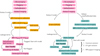 |
Fig. 1. Flowchart representing the similarities and differences between the pipeline presented in Homan et al. (2001, (left)) and our pipeline with DoG-HiT (right). Both pipelines illustrated here start post-calibration in AIPS. The data are processed in Difmap (pink), solved and adjusted for leakage terms in AIPS (yellow) and DoG-HiT in our pipeline, respectively (green), solved and applied for gain transfer, and finally imaged in full polarization. |
-
We complement the results obtained with the CLEAN algorithm by reconstructions using the DoG-HiT algorithm (Müller & Lobanov 2022, 2023b).
-
The self-calibration and D-term calibration are aimed to be improved. In particular, we self-calibrate using a phase-less imaging routine. Moreover, the D-terms are obtained by comparing the leakages recovered by a standard method (GPCAL, Park et al. 2021) and residual D-terms computed in a final step by DoG-HiT.
-
Finally, the gain transfer technique is implemented by a common data fidelity functional rather than a running median.
These updates address several limitations that a CLEAN-based approach may face: neither the convolved CLEAN image (which does not fit the data), nor the sample of delta components (which is not a physically reasonable description of the on-sky image), would be ideal for self-calibration, as neither can describe the data and perception of the image structure simultaneously (Müller & Lobanov 2023a). The latter might introduce systematics that tend to become frozen into the self-calibration (Pashchenko et al. 2023; Kim et al. 2024) and, hence, they may affect the much weaker Stokes V signal. Self-calibration and leakage calibration compare the model visibilities with the observed visibilities and optimize the gains and D-terms to maximize the match between these quantities. This procedure would return the true gain and leakage values once the true sky brightness distribution is known. However, as explained above, neither the CLEAN model (representing a biased nonphysical structure), nor the CLEAN image (which does not sufficiently fit the data) are well suited to performing the calibration of polarized intensities. As a consequence, performing the D-term calibration and gain self-calibration with the CLEAN components is expected to introduce small residual gain corruptions that may affect the much weaker circular polarization signal, in contrast to forward modeling techniques, which directly fit an on-sky representation of the image.
Furthermore, CLEAN is an inverse modeling approach; it is therefore impossible to separate the calibration of the RL offset or the amplitudes from the initial phase calibration, as well as the choices made interactively during the application of the algorithm. In contrast, recent forward modeling techniques relying on closure quantities only (e.g., Akiyama et al. 2017a,b; Chael et al. 2018; Broderick et al. 2020; Müller & Lobanov 2022; Müller et al. 2023; Albentosa-Ruiz & Marti-Vidal 2023; Mus et al. 2024a; Müller 2024) allow us to separate the phase and amplitude calibration, as well as to perform the self-calibration with an image structure, which has been recovered using only the gain-independent closure quantities. Due to these limitations, we opted for the forward modeling technique DoG-HiT, which may provide a more unbiased reconstruction of gains and leakages.
The core idea behind the gain transfer technique is that when averaging across multiple sources, the average circular polarization should vanish. This concept allows us to find smoothly varying RL gain ratios throughout the observation and consequently to disentangle the gain calibration from the circular polarization signal. The assumption of a statistically vanishing circular polarization signal is well-motivated on short baselines. However, the long baseline structure of the Stokes V signal, affected by, for example, local turbulence in the jet flow, may be more significant. This requires us to include the Stokes V structure in the calibration process, and consequently a stricter implementation of the gain transfer assumption. We achieved this by constructing a common data fidelity functional among multiple sources rather than applying a running median. We refer to Sect. 3.4 for more details.
It has only recently become possible to overcome these issues with the current advances in imaging and polarimetric methods for VLBI (e.g., Akiyama et al. 2017a,b; Chael et al. 2016, 2018; Broderick et al. 2020; Broderick & Pesce 2020; Arras et al. 2022; Tiede 2022; Müller & Lobanov 2022, 2023a,b; Müller et al. 2023; Mus et al. 2024a,b). In the following, we describe the individual steps of our calibration methodology in more detail and verify the methodology against established methods. To this end, we present exemplary comparisons and sanity checks for the 15 GHz data in the following subsections and the appendix.
3.2. Initial calibration and imaging
We followed the basic total intensity calibration procedure using the standard methods described in the AIPS cookbook. In particular, this includes corrections for instrumental delays, Earth orientation parameters, phase corrections for parallactic angles, amplitude corrections for digital sampling effects, fringe fitting, and solving for amplitude gain effects. We used Los Alamos (LA, antenna no. 5) as reference antenna when required.
After the initial calibration with AIPS, we averaged the data over a 10 s time-span, then we identified and marked the data points that deviate significantly from the norm in the imaging software Difmap. We detected data issues with the Brewster and Mauna Kea (MK) antennas at 23 GHz and consequently flagged these antennas at 23 GHz. For DoG–HiT to produce a best-fit Stokes I map, we provide total intensity maps a priori. For five of the nine target sources at 15 GHz, we used data observed during the same rough time frame (January 2022) from the publicly available MOJAVE data base. For the remaining four target sources (and for all target sources at 23 GHz), we created a Stokes I model using Difmap iteratively improving the flagging, calibration and image model.
DoG–HiT enhances the Stokes I image, specifically targeting compact emission characteristics. Initially, the approach entails an unpenalized imaging round as detailed in Müller & Lobanov (2022), utilizing the CLEAN image as the foundation. Subsequently, the DoG–HiT technique is employed, resulting in the preservation of the multi-resolution support to capture key features across scales. Finally, we self-calibrate the observation to the reconstruction. It is worth mentioning that the DoG–HiT procedure produces images by closure-only imaging and in a largely unsupervised way, that is, independent of the initial self-calibration and human bias. By processing only closure quantities rather than visibilities, fewer statistically independent observables are fitted, reducing the dynamic range in comparison to that achievable when fitting visibilities. However, this procedure recovers the image structure independently of the initial self-calibration, which has been identified as an important feature to ensure a bias-free circular polarization calibration further along the pipeline described here. To speed up the analysis and increase the accuracy, we added the χ2-metric to the amplitudes in the first round of the DoG-HiT procedure, and run the algorithm with a small number of iterations only to recover a first initial guess. Then this solution is used as an initial guess for the main DoG-HiT imaging which depends only on calibration-independent closure quantities. Moreover, DoG-HiT produces a physically reasonable super-resolved image that simultaneously fits the observed visibilities, hence alleviating possible biasing effects that may be introduced during the CLEAN self-calibration. The images presented in this work are the results of the DoG-HiT reconstruction following the additional calibration steps described below. The image structures were only determined up to a constant rescaling factor, fixed by the initially CLEANed total flux and totally absorbed in the amplitude calibration. This result is based on closure only imaging. However, since this effect is constant on all baselines, it does not affect the relative image structures in any polarization channel, that is, neither the total intensity contours and the polarized signal, nor the relative polarization fractions.
We verified the 15 GHz total intensity source structure obtained using DoG-HiT (Fig. B.5) with CLEAN images of all sources (Fig. B.4), both blurred to the same resolution. Apart from the absence of CLEAN artifacts, DoG-HiT reconstructs individual features within the jets more clearly than they appear in CLEAN. All nine total intensity maps of the observed sources are in overall good agreement between imaging methods. For more details, we refer to Appendix B.
3.3. Leakage calibration
After the cross-hand delay calibration using the task RLDLY in AIPS, the D-terms were finally calibrated during the full Stokes imaging in DoG-HiT (Müller & Lobanov 2022, 2023a,b). We solved for leakages in a two-step procedure: first, we obtained initial D-terms from the prior CLEAN images using GPCAL and then solved for residual D-terms with DoG-HiT in an iterative manner. The initial D-terms were estimated by the pipeline GPCAL (Park et al. 2021) which applies AIPS tasks (Greisen 2003). We applied the pipeline on three target sources and found the D-term calibration IF by IF with typical amplitudes of up to ±2%.
In Fig. B.1 we present the final leakages recovered by DoG-HiT compared to the ones recovered by GPCAL. The D-terms, both right-handed and left-handed, are rather small and match with reasonable accuracy. However, we also see slight differences between the methods, probably (but not necessarily) due to the possible bias within the CLEAN self-calibration procedure due to the use of a point-source model.
3.4. Gain transfer
The optimal Stokes I model for each source, along with the modified/unself-calibrated data, served as input for DoG–HiT. The pipeline involves resolving and fine-tuning compact polarization through the implementation of the DoG–HiT algorithm. To initiate the process, apriori D-term solutions obtained from GPCAL are applied. Instances of nonphysical high circular polarization are appropriately flagged for attention. Subsequently, both amplitudes and phases are calibrated within a 6-hour time frame.
During the calibration, we assumed the difference between right and left circular polarization ⟨RR − LL⟩ to be close to zero, indicating a small CP, vanishing statistically when averaging among various sources (but not necessarily on every source individually) – consistent with the strategy applied in, for example, (Homan & Lister 2006; Homan et al. 2018). Homan & Lister (2006) performed the calibration of the RL gain ratio on every source individually, also assuming a vanishing circular polarization signal. It is, however, impossible to separate the circular polarization signal from the self- calibration. Therefore, the gain solutions were smoothed across multiple sources by a running median over six hours. The calibration procedure is as follows: (i) iterative calibration; (ii) flagging of bad data points (strong polarization); and (iii) smoothing the calibration tables with a running median. This strategy implements the gain transfer assumption: the circular polarization signal of a single source is degenerate with the calibration procedure, and we can make the reasonable assumption that averaged across multiple sources the circular polarization vanishes.
For this manuscript, we attempted to implement this assumption more strictly. Due to the recent development of methods that realize VLBI imaging and calibration by, for example, convex optimization (ehtim, MrBeam, resolve) we can easily define a common data fidelity functional. We aimed to find a single solution for the RL-offset by fitting one (smoothly varying) solution to all data sets, that is, to a combination of the single data fidelity metrics of the single sources. The gain solution was computed with a correlation time length of 6 hours. To this end, we solved the minimization problem:
) \mathrm{d}\tau }\right\Vert,\nonumber \\ g^l_i(t), g^l_j(t)&\in \mathrm{argmin}_{g_i, g_j}\nonumber \\&\left\Vert{\int _{t-\Delta t}^{t+\Delta t} V^{\mathrm{LL}}_{ij}(\tau )-g_i^* g_j \mathrm{FFT}(\boldsymbol{I})([u_{ij},v_{ij}](\tau )) \mathrm{d}\tau }\right\Vert. \end{aligned} $$](/articles/aa/full_html/2025/05/aa47707-23/aa47707-23-eq7.gif)
Here, VRR and VLL denote the right handed and left handed parallel hand visibilities, gr/l the gains, i, j are indices counting the antennas, and Δt is the time-scale of the time average, that is, 6 hours. In contrast to self-calibration performed on every scan, we therefore aim to recover gain solutions that are consistent with the data over a long interval of times, and sources. In consequence, the gain curves are smoothed, similar to the effect achieved by a running median.
We show an exemplary set of amplitudes before application of the gain transfer technique in Fig. B.2 and the gain curves for all four IFs for three randomly selected antennas in Fig. B.3. The gain curves look reasonably smooth, as expected. However, we detect some larger phase swings at the edges of the observing window. This may be explained by the fact that the smoothed minimization is more challenging to compute at the edges of the observing window with fewer neighboring estimations, which would be used to construct a running median and smoothed gain curve. These times have thus been the target of a more thorough flagging, as outlined below.
We likewise computed the corrections iteratively. We fitted a gain solution to the data sets implying temporal smoothness, investigated the goodness of fit, and flagged bad data points. Then, we refined the gain solution and proceeded until convergence was achieved. We would like to highlight however, that the gain curve after each flagging is always applied to the leakage-calibrated original, non-R/L calibrated data set now with additional flags. Hence, the gain curve is only applied once for the final data set used for full Stokes imaging. The need for flags at this step in the analysis stems from multiple motivations. First, we performed closure-only imaging in the previous step with DoG-HiT. The typical iterative mapping, flagging and self-calibration done interactively with CLEAN was therefore not applied which leaves a bigger need to do this flagging at latter steps of the analysis. Second, as outlined above, at the edges of the observing window, we need to apply extra caution to the gain solutions. This flagging has been performed manually. In Fig. B.2, we present a typical baseline that has been flagged for early times. We discuss the heuristics of our flagging procedure in more detail in Appendix B.
Finally, we found a single, temporally smoothed gain curve that reflects the best compromise in fitting the individual data fidelities with this procedure. We present the gain curves per IF for three randomly selected antennas in Fig. B.3. Our final circular polarization images in both frequencies are presented in Figs. 4 and A.2.
For comparison (and to validate the pipeline), we also calibrated all sources using the strategy described in detail in Homan & Lister (2006). The resulting 15 GHz circular polarization maps are shown in Fig. B.6. The results are remarkably similar to those obtained by DoG-HiT, with notable exceptions. 1243–027 has a bi-modal core structure in circular polarization, which is rarely reflected with the second calibration technique. This shows that the exact structure of these bi-modal signatures is uncertain, and should not be over-interpreted. Further, some significant differences can be seen for 1127+145 and 1546+027 where the circular polarization signal appears less structured and noisy when using DoG-HiT.
In our sample at 15 GHz, only one out of nine sources has a negative sign. This may point towards a potential issue during the application of the gain transfer technique, in detail, its basic assumption may be violated. As an additional validation test, we inspected this behavior and have observed that incorporating longer baselines increased the average circular polarization deviating from zero. This occurs because self-calibration incorporates all baselines, and some sources (e.g., 0149+218, 0528+134, 0748+126, 1127–145) are resolved. Our imaging process, being more sensitive to small-scale structures, differs from classical CLEAN, and longer baselines contribute significantly to the gain calibration as well. Thus, the assumption that CP averages to zero across sources applies not only to short but also to long baselines.
To validate this, we flagged the longest baselines (larger than 0.2 Gλ) during gain transfer and re-imaged at 15 GHz. This produced a more uniform CP distribution (four sources negative, five positive). These results, along with smoothed gain curves for Fort Davis, Kitt Peak, and St. Croix, are detailed in Fig. B.3. While most gain curves were consistent, flagged data sets showed smoother gains, particularly reducing the edge-related issues in potentially problematic time intervals mentioned above.
We show our final CP maps when using these gains in Fig. B.7. For most sources, the relative CP structures remained consistent to the level of showing the same structural features (e.g., single-peaked or double peaked, and trend of CP along and transverse to the jet), except for 1243 and 1546, which varied significantly across calibration methods. This suggests their CP signals may be influenced mainly by gain calibration. Notably, 1243 and 1546 had the sparsest uv-coverage, making them the weakest constrained sources.
3.5. Full Stokes imaging
Since gain- and D-term calibration (and particularly the corresponding flagging) may have affected the Stokes I observables, we refined the total intensity imaging. We refined the total intensity images with a small step size gradient descent algorithm to fit the flagged and calibrated data set, starting from the earlier computed Stokes I solution. Following this step, the linear polarization imaging is subjected to the DoG–HiT procedure as described in Müller & Lobanov (2023b).
The imaging process is further extended to address circular polarization using DoG–HiT in the same way, that is, by fitting the Stokes V visibilities, but only varying the parameters in the multiresolution support (following the philosophy in Müller & Lobanov 2023b). In other words, we are only using the multiscale basis functions that were found to be of statistically significant to represent the total intensity to model the linear and circular polarization. A five-round iterative refinement cycle was established for the linear and circular polarization and the residual D-term calibration. This comprehensive approach aims to progressively enhance the precision and quality of the (linear) polarization results.
Residual RL offsets may still be present in the data even after these imaging and calibration steps, especially on long baselines where the gain transfer assumption is potentially inappropriate. This can result in pointy, noisy reconstructed circular polarizations, especially when recovering images at super-resolution. We refined the imaging of Stokes V with the de-noised, compact Stokes V reconstructions. To this end, we implemented manual procedures in DoG–HiT that are described in the following paragraphs.
Based on the 1%-contour of the Stokes I image, a mask delineating a compact and luminous region was created. This mask was then applied to the Q, U, and V polarization components. Moreover, the Stokes V structures were blurred using a Gaussian filter.
Following these adjustments, the final images were generated by minimizing the χ2-metric to the fully calibrated Stokes V visibilities with a gradient descent approach stopped by the discrepancy principle starting from the blurred, and masked circular polarization images created in the last step. To this end, we allowed only pixels within the 1% mask to vary.
In Fig. 2, we show the final calibrated circular polarization amplitudes and image fits. The observations are fitted adequately with smooth (regularized) solutions, indicating a successful fit given the various constraints imposed on the polarimetric deconvolution.
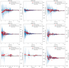 |
Fig. 2. Final calibrated and flagged Stokes V amplitudes as a function of uv-distance (blue points) and the respective fit (red points). |
The final images show a range of anti-symmetric peaks in CP which may be introduced to the image by phase calibration errors. Homan & Lister (2006) detected similar structures, and proposed to apply a last phase self-calibration step at the end to remove them from the images, assuming VRR, VLL = FFT(I). To test whether this is the case, we applied this strategy as well, and show the reconstructions after a final self-calibration step in Figs. B.8 and B.9 as well.
Further, we would like to note that a CLEAN-based pipeline may be also prone to over-align phases in general. This is because the phase calibration cannot be separated from the amplitude calibration, and the initial phase calibration is necessarily performed during the Stokes I imaging on a starting model, or a model with only a few components. That may introduce phase solutions that are too much aligned on a rather simplistic symmetric structure early on the analysis, something that may be challenging to correct afterwards during the gain-transfer. Moreover, we selected sources that were expected to show a rich CP.
3.6. Uncertainty estimation
In Table 1, we present the achieved RMS noise for the reconstructions with DoG-HiT for a comparison with literature results. We note that the DoG-HiT procedure does not minimize a residual in the classical sense (but fits data properties by forward modeling), and works with the closure quantities rather than the visibilities (which do not form a dirty map/dirty beam deconvolution pair due to the non-linearity of the forward operator). To define a quantity akin to the residual RMS commonly used in VLBI, we here report the rms(FFT−1[V−FFT(I)]), where I is the recovered image, and V are the observed visibilities. However, we would like to note that potential over-alignment of the phases to the closure-only fit, the extent of flagging, and the explicit involvement of gridding uncertainties (that are still present in the CLEAN residual, and are typically drastically reduced by multiple major loop iterations) affect the RMS. Moreover, overfitting of the noisy structure would show up as a reduced noise level, with the noise-structure imprinted in the forward model. We have evaluated our images visually by eye to assess that latter did not appear, with the notable exception of 0149+218 at 23 GHz, which shows an extended structure around the core-jet structure that is most likely attributed to imaging or calibration artifacts rather than true image structure. In this case, we rather applied the peak of non-true image structure rather than the RMS. All these drawbacks should be taken into account when comparing to noise levels reported by CLEAN. At 15 GHz we typically achieve an RMS level of ∼0.1 mJy/beam which lies well in the ballpark that may be expected by VLBA observations at this frequency, with 0059+581 as notable exception. For 23 GHz, we typically score RMS errors of a few mJy/beam, leading to dynamic ranges of ∼500 − 2000. We note more variety across the sources in the RMS at 23 GHz, and therefore present the RMS achieved by the CLEAN data reduction done in the first step of the data analysis as well for comparison. The RMS error with DoG-HiT may be underestimated, especially for 0528+134.
The CP reconstruction is strongly affected by the gain calibration. A first idea of the relative uncertainty of the recovered features may be available by comparing the recovered features with different calibration techniques, that is, by comparing Figs. 4, B.6, B.7 and B.8 at 15 GHz, and Figs. A.2 and B.9 at 23 GHz.
For an analytic approximation to the errors in the CP reconstructions, we apply the scheme proposed by Homan et al. (2001). The residual RMS of the CP reconstruction is typically underestimating the true uncertainty due to the uncertainty in the gains. Homan et al. (2001) therefore suggested to estimate the uncertainty from three components: the uncertainty in the determination of the smoothed gains quantified by the scan-to-scan variations of the gain solutions across all sources, the uncertainty in true circular polarization of the calibrator (estimated by the RMS of the apparent CP), and finally uncertainties introduced by uncorrected rapid variations in the gains (estimated for every source by variations of the gain solutions in time). For more details, we refer to Homan et al. (2001). We note that our calibration technique differs in some details from the calibration technique this uncertainty estimation was tailored to. In particular, we originally do not compute gain solutions at every scan that we smooth in post-processing, and that could be used to estimate the scan-to-scan variations for the uncertainty estimate. Rather, we tried to fit a smooth curve directly, compare our discussion in Sect. 3.4. However, the two approaches are philosophically similar. Therefore, we recomputed the gain solutions and running median calibration, as proposed in Homan et al. (2001) at both frequencies, and adapted the related error estimates for our results as well.
4. Results
Full Stokes maps for all target sources are displayed in Figs. 3–A.2, each convolved with a Gaussian beam. The beams are shown in the lower right corner of each map, while their sizes can be found in Table 1. Our records of total intensity and polarization measurements in both 15 GHz and 23 GHz are summarized in Table 1 and the fractional measurements are presented in Table 2. In Table 1, comprehensive data are provided for total intensity (Stokes I), linear polarization (LP,  ), and circular polarization (CP, Stokes V) at the peak of each map. The peak total intensity in Jansky (Jy) for all nine observed blazar sources range between 0.36±10−5 ≤ I ≤ 1.7±1.4 × 10⁻³ Jy/beam for 15 GHz observational data and 0.33±2 × 10⁻⁵ ≤ I ≤ 2.9±7.8 × 10⁻³ Jy/beam at 23 GHz (see upper left corner in each map in, e.g., Figs. 3 and A.1)5 The total intensity peak value remains consistent at both 15 GHz and 23 GHz wavelengths. For a comparison to our values presented in Table 1, see the MOJAVE data archive. Evident jet structures are observed in 0149+218, characterized by a prominent bright spot to the north. An extended jet structure is further observed in 0528+134, 0748+126, and 1127–145. Notably, at both frequencies a counter-jet is newly observed in 0149+218 to the south and in 2136+141 to the east at 23 GHz, marking the first occurrence of this phenomenon in these sources that is mentioned in a publication. The Quasar 0149+218 has a jet speed of (14.29 ± 0.76) c (Lister et al. 2019) – a strong argument against the visibility of a counter-jet. However, the Bordeaux VLBI Image Database shows a very similar structure to the map displayed in their database (BVID 2008).
Fractional polarization.
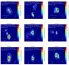 |
Fig. 3. Reconstruction of data from 6–7 Jan. 2022 for nine target sources: 0059+581, 0149+218, 0241+622, 0528+134, 0748+126, 1127–145, 1243–072, 1546+027, and 2136+141. The figure shows maps for each source in linear polarization at 15 GHz (color coding: blue-low and red-high). The total intensity is indicated in white contours on each map. The contours are the [0.1%,0.2%,0.4%,…,25.6%,51.2%] levels of the peak brightness. The orientation of the linear electric vector position angle is plotted as white ticks, the total polarized intensity by the colormap. An individual convolution beam (natural weighting) is shown in the lower right corner of each map. The field of view is shown by the scale with 3 mas in the lower left. |
The core component of the Quasar 0149+218 shows a cross-like feature usually not seen in archived CLEAN images. To a smaller degree, we see the same structure in the Quasar 0059+581. Since also the jet in the quasar 0149+218 shows more fine structure (components) than in usual images derived with CLEAN (although that may be explained when DoG-HiT is more sensitive to small scale structure), we add some discussion of this phenomenon here. We note that with DoG-HiT we apply a non-linear minimization scheme fitting the amplitudes and closure quantities, rather than an inverse modeling scheme working with the visibilities. In Fig. B.10, we show the reconstructions in total intensity with CLEAN, and DoG-HiT. Moreover, we show the reconstruction achieved by DoG-HiT when only fitting closure phases and closure amplitudes, and the reconstruction achieved when fitting only closure quantities with a LASSO approach. LASSO assumes that the model is sparsely represented in the pixel domain, namely, it imprints the same assumption that goes into CLEAN (although it still differs significantly from CLEAN as a forward modeling approach). We see that the LASSO reconstruction is relatively similar to the DoG-HiT reconstruction using the same data properties, with the difference that latter one filtered out the over-resolved core. That may indicate that the cross-like structure, as well as the spurious components in the jet are not introduced by the wavelet approach, but may be caused by the data fidelity terms.
We see core components to the east and to the west for all reconstructions that utilize closure quantities, in contrast to CLEAN which works with the visibilities. When blurred to the CLEAN resolution the structure (especially in the jet) resembles the CLEAN one, which is natural. The features are more prominent when we factor in amplitudes, rather than only closure quantities. There may be two possible interpretations here. First, it could be that there are non-station-based errors that get more highlighted and projected to the images when we rely on the closure quantities only, or the statistics is just smaller introducing spurious artifacts (but then the potential artifacts should be less prominent when using amplitudes additionally). Second, it may be that the imaging with DoG-HiT (which is robust against any phase corruptions) may give rise to more fine structures that are iteratively removed from the CLEAN reconstructions, for example, when the phases in the early iterations are potentially too much aligned around the dominant core.
Ultimately, both solutions fit the data. In this manuscript, we go on with the solution derived by DoG-HiT (derived from the amplitudes and closure quantities) due to consistency with the other sources, and since a manual inspection of the amplitudes did not look suspicious to us. For reference, we show in Fig. B.11 the polarization results that we obtain when using only closures. The linear polarizations match very well. However, we observe quite significant changes in circular polarization, although not changing our interpretation.
4.1. Polarized intensity maps
Figure 3 shows the linear polarization at 15 GHz overplotted with both the contours in total intensity and EVPAs as white ticks. The same plotting scheme is illustrated in Fig. A.1 for 23 GHz. The circular polarization maps at 15 GHz and 23 GHz are presented in Figs. 4 and A.2, respectively. In all observed blazars the peak of the Stokes I map corresponds to the compact and resolved VLBI core. The VLBI core is consistently linearly polarized. Minor discrepancies arise between circular polarization and the peak in total intensity specifically within the VLBI core (with no impact on the extended jet structure). This discrepancy is likely attributed to the phase calibration process (detailed in Sect. 3), which could potentially introduce a minor positional shift between the location of circular polarization and the Stokes I peak. The overall values for the fractional linear and fractional circular polarization [%] are in a range of 0.53±0.21 ≤ ml ≤ 4.34±0.4 and 0.14±0.19 ≤ |mc|≤0.65±0.21 at 15 GHz, and 0.72±0.2 ≤ ml ≤ 6.22±0.2 and 0.22±0.2 ≤ |mc|≤1.5±0.22 at 23 GHz. For reference and details see Table 2.
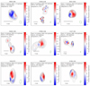 |
Fig. 4. Circular polarization imaging results from 6–7 Jan. 2022 for nine target sources: 0059+581, 0149+218, 0241+622, 0528+134, 0748+126, 1127–145, 1243–072, 1546+027, and 2136+141. The figure shows maps for each source in circular polarization at 15 GHz (colorcoding: blue/red negative/positive). The total intensity is indicated in white contours on each map at levels of [0.1%,0.2%,0.4%,…,51.2%] of the peak brightness. An individual convolution beam is shown in the lower right corner of each map. The field of view and source size are shown by the scale, with 3 mas in the lower left. |
4.1.1. Polarized structure
At 23 GHz, the peak of linear polarization in the target source 0748+126 is displaced from the VLBI core with respect to the total intensity I in the linear polarization map (see Fig. 3). This behavior for the linearly polarized structure is observed in 0149+218 (23 GHz), 0241+622 (mainly 15 GHz), 0528+134 (15 GHz), 0748+126 (23 GHz) and 2136+141 (15 GHz).
As for the circular polarization, there is a dominant pattern of a two-sign circular polarization (CP) structure at 23 GHz (Fig. A.2), which contrasts with a positive trend at 15 GHz (Fig. 4). This dominant sign alteration, however, exhibits hints in the sources 0241+622 and 0748+126. In the case of the blazars 0059+581 and 2136+141, a consistent and predominantly one-signed radio core is observed across both 15 GHz and 23 GHz. Most of the sources show an alignment between the circularly polarized intensity peak and the total intensity structure. This suggests the mechanism producing CP works effectively at the jet’s base, near the τ = 1 surface, where τ represents optical depth (Homan & Wardle 1999). It’s crucial to remember that the ‘core’ as the optically thick jet base (Blandford & Königl 1979) is theoretical and matches the observed “core” only in high-resolution observations (Vitrishchak et al. 2008). Generally, the position of the V peak is influenced by the magnetic field strength and electron density, indicating an expected strong CP signal. One scenario could be that the circular polarization peak emerging slightly before the I peak signals the upcoming emergence of a new VLBI component (Vitrishchak et al. 2008).
In general, the fractional CP tends to be higher at 23 GHz compared to 15 GHz (see Table 1). We are confident that these findings are not the result of observational artifacts. When analyzed collectively or individually, the 23 GHz  values exceed those at 15 GHz, as shown in Table 2. The observation that mc increases with frequency in several sources, consistently showing higher values at 23 GHz than at 15 GHz frequency, aligns with Wardle & Homan (2003). They suggested that CP, whether from synchrotron radiation or Faraday conversion in a Blandford & Königl (1979) jet, could show an inverted CP spectrum, mc ∝ ν. This implies our measurements might reflect the intrinsic inhomogeneity of the jet affecting the observed CP and its spectrum. Moreover, the complexity increases as core CP measurements could blend CP contributions from various regions within the core and the innermost jet, a phenomenon directly observed in 3C 84 (Homan & Wardle 2004).
The sources 0059+581, 0149+218, 0748+126, and 1127–145 show an elongated EVPA structure along the jet direction at 15 GHz (see Fig. 3). For 0528+134 (and 1127–145 to some extent) we observe the EVPAs to be perpendicular to the jet direction at both frequencies (see Figs. 3 and A.1).
4.1.2. Amplitude of polarization
We detect circular polarization (and linear polarization) in all nine target sources. The distribution of the peak values of linear and circular polarization is consistent throughout all sources; specifically, the amplitude in linear polarization (Stokes Q and U) is consistently higher than the circular polarization amplitude (Stokes V). The ratio of the fractional values of linear polarization, ml, to circular polarization, mc, vary to a greater extent6. Then, 0059+581, 0149+218, 0748+126, 1127–145, 1243–072, (1546+027), and 2136+141, have significantly higher fractional linear polarization ml values compared to fractional circular polarization, mc, at 15 GHz and 23 GHz. Overall, there is no clear trend for either frequency nor in the fractional LP when comparing 15 GHz and 23 GHz.
4.2. Super-resolution
DoG-HiT achieves super-resolution by combining the significant advantages of regularized maximum likelihood reconstructions, which super-resolve structures, with the CLEAN method, which provides high dynamic range sensitivity to extended structures. For CLEAN, the model that is fitted to the visibilities is a list of δ-components which is a nonphysical representation of the on-sky image. Therefore, we need to convolve the model with the clean beam for a proper representation of the image. Regularized maximum likelihood reconstructions, multiscalar CLEAN variants, or Bayesian approaches which fit smoothed, spatially correlated functions to the visibilities may not need this final convolution. The fitted model itself can be already seen as a proper representation of the sky brightness distribution, a potential way towards super-resolution under the limitation that the algorithms may pick up noisy small-scale features. We refer the reader to Honma et al. (2014) for an illustrative discussion of this point, and to Müller & Lobanov (2023a) for a demonstration in a CLEAN-based environment. Remind from Sect. 3 that this fact was one of the main motivations for the imaging and calibration strategy applied in this manuscript.
Without applying a Gaussian beam convolution (in contrast to Figs. 3–A.2), we obtained a super-resolved image (see Fig. 5) that fits the observed visibilities similarly as the list of δ-components in CLEAN. We chose the blazar 0528+134 at 15 GHz as an example, since the source shows the richest structural features along the jet (see Fig. 4). The blurred map (fourth panel in Fig. 4) matches the reconstructed 15 GHz map available in the MOJAVE data base quite well, compare also Figs. B.4 and B.5. The difference that we achieve by illustrating the super-resolved jet in Fig. 5 is that it shows two distinct features further upstream, whereas the MOJAVE image would resolve a single upstream (polarized) feature. This suggests that the improvements made to our pipeline allow us to resolve distinct features at lower frequencies.
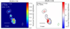 |
Fig. 5. Reconstruction of data from 6–7 Jan. 2022 for the quasar 0528+134. The images show the resolved maps of: linear polarization at 15 GHz (color coding: blue-low and red-high) in the left panel. The total intensity is indicated in white contours. The linear electric vector position angle is plotted as white ticks. Right: circular polarization (colorcoding: blue-negative and red-positive). The total intensity is indicated in white contours. |
In this paper, we primarily report the net polarization, rather than the total polarization fraction due to its advantages in the scientific interpretation. Both quantities are expected to match for marginally resolved sources with a preferred EVPA pattern, but differ the more resolved and scrambled the EVPA pattern appears, as is the case here. To ease comparison with other observations, we also report the total polarization fraction in Fig. 5 which is significantly higher than the net polarization.
Past analyses of the trajectories of individual moving features show that the bend is more pronounced closer to the core and gradually straightens out farther away (Britzen et al. 1999). Curvature on small angular scales has been observed in numerous other sources, suggesting that it is a common phenomenon in AGN (e.g., Zensus et al. 1995 for 3C 345 and Wagner et al. 1995 for PKS 0420–014). A possible explanation for the observed “wiggling” of the core region is the ejection of moving features along different, but straight trajectories, resembling ballistic motion (e.g., Jorstad et al. 2017). The EVPAs are oriented perpendicular to the jet’s direction, matching an underlying poloidal magnetic field morphology (Kramer & MacDonald 2021) and being consistent with the 43 GHz observations presented in Palma et al. (2011).
5. Discussion
It is imperative to highlight improvements in the imaging and calibration procedure that could potentially account for the cases of high circular polarization. In previous works (Homan & Wardle 1999) and in the present case, it was not possible to detect reliable resolved CP in AGN. The usual level of detectable CP was around 0.1% (see early studies in, e.g., Weiler & de Pater 1983; Komesaroff et al. 1984). Similar to Homan & Wardle (1999) and following years we cannot draw any conclusions on any of the mechanisms involved in the production of CP; however, with our methods and the application and comparison of their method in our dataset, we can interpret the most favorable magnetic field configurations. In particular, the accuracy of Stokes V strongly hinges on meticulous calibration. To be more precise, our self-calibration is anchored in a physical model, as opposed to relying on a potentially non-physical model of CLEAN (delta) components. This adjustment results in potentially more accurate gains.
Figure 2 shows the amount of detected circular polarized emission over the uv-distance. It further stresses that the observed circular polarization is primarily detected on shorter baselines. The observed data (in blue) are well aligned with the reconstructed model (in red) within the noise budget. There is no significant trend over the distance, nor are there any major outliers within our calibration method.
While the closure phases for RR and LL remain resilient to variations in antenna gains, they could potentially be affected by instrumental polarimetric leakage. However, the effect of uncertainties in D-terms is significantly more pronounced in cross-hand visibilities compared to parallel-hand visibilities (Smirnov 2011). Consequently, this implies that instrumental polarization exerts a comparatively lesser effect on Stokes V in comparison to its impact on Stokes Q and U. For our data, we hence stress again that the Stokes V signal is robust and reliable. The rotation of the EVPAs could slightly change depending on the solution of the leakage terms.
We need to comment, however, that for the two sources 1243–072 and 1546+027, the recovered CP structure depends strongly on the calibration method and is most likely driven by gains. The interpretation of the recovered maps is based on the morphologies in LP and CP across the two frequencies. We need to highlight however as a limiting factor that the CP signal at 23 GHz suffers from large gain-driven uncertainties with only a few significant detections.
The presence of substantial fractional circular polarization, reaching up to  in our dataset at both frequencies, exceeds previously observed circular polarization rates documented by, for instance, Homan et al. (2001), Homan & Lister (2006)7 using the VLBA at 5 GHz or by MOJAVE observations with the VLBA at 15 GHz (Homan & Lister 2006, here CP was around 0.3 percent). We agree with their conclusion that the overall circular polarization value tends to increase at higher frequencies (see also Vitrishchak et al. 2008).
Although the observed circular polarization could theoretically originate from intrinsic CP via synchrotron radiation, certain observed mc values are too elevated to justify by this means alone, necessitating either unrealistically strong or exceptionally orderly magnetic fields. In some instances, mc values exceeding 1% have been noted (Homan & Lister 2006; Homan & Wardle 2004; Vitrishchak et al. 2008). Another case of remarkably high fractional circular polarization was detected in 3C 84, exceeding mc = 3% (Homan & Wardle 2004). Therefore, it is likely that an alternative mechanism is at work in certain scenarios. This mechanism is thought to be Faraday conversion, transforming linear polarization into circular polarization within a magnetized plasma (Gabuzda 2021; O’Sullivan & Gabuzda 2009).
Most of our sources exhibit stable degrees of fractional linear polarization over the last years (monitored by the MOJAVE program). Eight out of nine sources remain consistent in the peak brightness of the linear polarization, P, the polarization angle, and the degree of polarization,  , compared to the archival data collected over several years to decades in the MOJAVE data archive.. The only exception is 0149+218, which shows a dimmer peak in our data. Furthermore, 0241+622 has no previous information on EVPA in the MOJAVE database, however, the values of our polarization study are comparable with observations performed in 2007. The offset between the total intensity and linearly polarized intensity seen in 0528+134 is consistent with polarized maps in the MOJAVE dataset. For the blazars 0748+126 and 1127–145, our study results in a lower peak brightness in Stokes I. In the case of 0059+581 and 2136+141, the jet structure appears to be oriented further to the south (rather than west) in 15 GHz compared to its appearance in 2013 and 2023, respectively (see 0059+581 and 2136+141 in the MOJAVE data archive).
Kramer & MacDonald (2021), Kramer et al. (2024) provided an analysis on how the magnetic field morphology affects the polarized synchrotron emission within the recollimation shock (VLBI core) and the extended jet structure. They found a centrally highlighted VLBI core and a single sign in CP for a purely poloidal magnetic field. In contrast to that, a purely toroidal magnetic field would result in an edge-brightened jet, a bi-modal EVPA pattern (where the EVPAs tend to align with the jet’s direction of motion within the spine), and a two-signed CP structure within both the VLBI core and the jet. A helical magnetic field combines these morphological characteristics.
In the context of theoretical forecasts, a tendency toward a favored magnetic field orientation becomes evident within the extended jet emission of, for instance, 0241+622; its polarized structure suggests an underlying toroidal magnetic field structure. This conclusion is supported by two observations at 15 GHz, namely, a bi-modal pattern of EVPA (see Fig. A.1) and the presence of two signs in CP (see Fig. A.2). The jet structure in 0528+134 observed at 15 GHz in super-resolution (see Fig. 5) exhibits characteristics that are aligned with a helical or rather poloidal magnetic nature.
The blazar sources 0059+581, 0748+126, and 1127–145 are in agreement with a helical magnetic field morphology. The EVPA tend to follow the jets motion (even when bending), however, the central peak of the linear polarization is slightly off-center from the total intensity peak (see, e.g., Fig. 3).
For the radio core, the configuration in 0528+134, 0748+126, 1127–145, and 2136+141 presents traits indicative of a helical or toroidal magnetic field structure, supported by a double sign in CP in either frequency (except for 1546+027 which is showing the bimodality only at 15 GHz). We note, however, that the bimodality observed for 1243–072 and 1546+027 are not robust against changing the calibration strategy. Consequently, the interpretation of a toroidal magnetic field configuration may be an over-interpretation for this source. Asymmetric bimodal structures may be caused by phase errors (Homan & Lister 2006). However, we trust the found source structures for the other sources due to their robustness against multiple calibration techniques (except 1243–072 and 1546+027), and against a final self-calibration as suggested in Homan & Lister (2006). An offset between the linear polarized intensity peak and the total intensity peak is visible in, for instance, 0241+622 and 2136+141, which is favored in a helical treatment of the magnetic field (Gabuzda 2018, 2021). This aligns with synthetic polarized emission maps presented in Kramer & MacDonald (2021). When focusing on the radio core of the sources 0059+581 or 0748+126 an emphasis can be placed on a purely poloidal magnetic field structure. This is summarized in Table 3.
Preferred magnetic field morphology.
For quite some time, it has been established that the circular polarization sign within a specific AGN tends to remain consistent over extended periods, often spanning years or even decades, as highlighted by Homan & Wardle (1999). However, limited information has been available concerning the frequency-dependent behavior of the CP sign. Vitrishchak et al. (2008) findings reveal that out of nine AGN where CP was detected at both 15 GHz and 23 GHz, eight consistently displayed the same sign, with 2251+158 being the exception. Among the six AGN where CP was detected at both 23 GHz and 43 GHz, four exhibited changes in sign between these two frequencies (namely, 0851+202, 1253–055, 1510–089, and 2251+158). We observe the switch in sign for three to five sources as described in Sect. 4.1.1. The occurrence of alterations in the CP sign as the frequency shifts from 15 GHz to 23 GHz implies the influence of optical depth effects. This observation suggests that the sampled regions are likely to be optically thin. In particular, we would like to draw attention to the blazar 0241+622 which experiences a complete switch in sign of CP structure from 15 GHz to 23 GHz. The interpretation and findings in CP is supported by the offset in EVPA rotation when both frequencies are compared. However, optically thick regions favor the generation of CP with a specific sign influenced by the magnetic field configuration. As the jet transitions to being optically thin, CP may weaken or reverse due to changes in the plasma’s characteristics. We are therefore cautious with our interpretation of the magnetic field, however, we do interpret favored magnetic field configurations with a conclusive comparison to synthetic polarized emission maps based on thermal plasma simulations.
6. Conclusion
We employed an advanced imaging algorithm using the imaging software DoG-HiT, which potentially shows improvements in the reconstruction of compact structures in an unbiased way. Notably, DoG-HiT performs polarized gain calibration using the compact Stokes V structure free of biases induced by CLEAN. Our calibration method reveals no misleading trends in the right-or left-handed circular polarization at different distances and no major outliers, reinforcing the robustness and reliability of the Stokes V signal in our data.
Following Gabuzda (2018), we can concur that magnetic fields with a toroidal component or with a helical nature are the most plausible explanations for the extended jet structures (see Table 3). Our analysis leads us to the conclusion that circular polarization serves as a powerful tool for elucidating the intrinsic magnetic field morphology of jetted AGN. Through this approach, we have been able to associate most of the sources with specific intrinsic magnetic field morphology. In particular, we have been able to explore whether the magnetic field is poloidal or toroidal in nature and to identify a favored composition within each. The findings extracted from our study can be summarized as follows:
-
The polarized structure, level of polarization, and EVPA orientation over time compared to archival MOJAVE data is very robust (see Fig. 3).
-
Theoretical predictions favor specific magnetic field orientations within the extended jet structures of the blazar sources (Kramer & MacDonald 2021).
-
The changes in the (dominant) CP sign as the frequency transitions from 15 GHz to 23 GHz suggests the influence of optical depth effects (cf. Figs. 4 and A.2).
-
Two blazar sources show signs of a newly manifested counter-jet structure in total and linearly polarized intensity: 0149+218 to the south (15 GHz; carrying negative CP) and 2136+141 to the east (23 GHz; negative sign in CP).
-
We reconstructed a resolved 15 GHz map of the blazar 0528+134, which shows super-resolved components at lower observational frequency than previously observed.
-
We avoided relying on a potentially non-physical model of CLEAN components by anchoring our self-calibration to a physical model.
-
Our polarization calibration method departed from previously applied methods that assume V = 0; instead, we integrated the compact Stokes V structure.
To strengthen the reliability and authenticity of the observed and reconstructed polarized signal, we intend to compare the VLBI data, accounting for leakage terms of each antenna, with the levels of polarized emission obtained through single-dish measurements. To achieve this validation, we intend to utilize data from the G-GAMMA/QUIVER program (full Stokes, multi-frequency radio monitoring of Fermi blazars with the Effelsberg telescope, Angelakis et al. 2019) and the Polarimetric Monitoring of AGN at Millimeter Wavelengths with the IRAM 30 m telescope program (POLAMI, Agudo et al. 2018), focusing on quasi-simultaneous observations that align with our study. This approach will also yield essential information about on the absolute electric vector position angle.
To make strong assumptions on a preferred magnetic field, a statistical analysis would be necessary. This could, in principle, be conducted by using the archival MOJAVE data. In addition, to further test and verify the favored magnetic field morphology for the different sources, we plan to compare synthetic transverse intensity profiles with those obtained from the sources presented in this work. To stress the conclusions drawn on the optical depth, a future work will focus on the analysis of the spectral index maps obtained between 15 GHz and 23 GHz.
For a detailed listing visit the MOJAVE 2 cm Survey Data Archive.
We are aware of additional affects, and we discuss opacity affects among others later in the paper. However, we chose to perform a specific comparison between our observations and models applied in Kramer & MacDonald (2021).
Acknowledgments
J. A. Kramer and H. Müller have contributed equally to this work. The authors thank J. D. Livingston for his intense research and fruitful discussion on polarization. We thank J. Kim for his insights on Bayesian imaging techniques on polarized data. We acknowledge I. Myserlis and N. R. MacDonald for their contribution to the observational proposal. We are grateful for D. Pesce’s insights on the calibration steps. The analysis was performed with the software MrBeam8 which is partially based on ehtim9, regpy10 and Wise11. J. A. Kramer is supported for her research by a NASA/ATP project. The LA-UR number is LA-UR-24-22726. H. Müller acknowledges financial support through the Jansky fellowship program of the National Radio Astronomy Observatory. J. Röder acknowledges financial support from the Severo Ochoa grant CEX2021-001131-S funded by MICIU/AEI/ 10.13039/501100011033. This research was supported through a PhD grant from the International Max Planck Research School (IMPRS) for Astronomy and Astrophysics at the Universities of Bonn and Cologne. The observations presented are conducted with the Very Long Baseline Array (VLBA) operated by National Radio Astronomy Observatory (NRAO) and correlated at the NRAO correlator in Soccoro. NRAO is a facility of the National Science Foundation operated under cooperative agreement by Associated Universities, Inc. This work is part of the M2FINDERS project which has received funding from the European Research Council (ERC) under the European Union’s Horizon 2020 Research and Innovation Program (grant agreement No 101018682).
References
- Agudo, I., Thum, C., Molina, S. N., et al. 2018, MNRAS, 474, 1427 [NASA ADS] [CrossRef] [Google Scholar]
- Akiyama, K., Ikeda, S., Pleau, M., et al. 2017a, AJ, 153, 159 [NASA ADS] [CrossRef] [Google Scholar]
- Akiyama, K., Kuramochi, K., Ikeda, S., et al. 2017b, ApJ, 838, 1 [NASA ADS] [CrossRef] [Google Scholar]
- Albentosa-Ruiz, E., & Marti-Vidal, I. 2023, A&A, 672, A67 [NASA ADS] [CrossRef] [EDP Sciences] [Google Scholar]
- Angelakis, E., Fuhrmann, L., Myserlis, I., et al. 2019, A&A, 626, A60 [NASA ADS] [CrossRef] [EDP Sciences] [Google Scholar]
- Arras, P., Bester, H. L., Perley, R. A., et al. 2021, A&A, 646, A84 [NASA ADS] [CrossRef] [EDP Sciences] [Google Scholar]
- Arras, P., Frank, P., Haim, P., et al. 2022, Nat. Astron., 6, 259 [NASA ADS] [CrossRef] [Google Scholar]
- Blandford, R. D., & Königl, A. 1979, ApJ, 232, 34 [Google Scholar]
- Britzen, S., Witzel, A., Krichbaum, T. P., Qian, S. J., & Campbell, R. M. 1999, A&A, 341, 418 [Google Scholar]
- Broderick, A. E., & Pesce, D. W. 2020, ApJ, 904, 126 [NASA ADS] [CrossRef] [Google Scholar]
- Broderick, A. E., Gold, R., Karami, M., et al. 2020, ApJ, 897, 139 [Google Scholar]
- BVID 2008, https://bvid.astrophy.u-bordeaux.fr/source/49/0149+218.html [Google Scholar]
- Chael, A. A., Johnson, M. D., Narayan, R., et al. 2016, ApJ, 829, 11 [Google Scholar]
- Chael, A. A., Johnson, M. D., Bouman, K. L., et al. 2018, ApJ, 857, 23 [Google Scholar]
- Contopoulos, I., Gabuzda, D., & Kylafis, N. 2015, in The Formation and Disruption of Black Hole Jets, (Springer International Publishing Switzerland), Astrophysics and Space Science Library, 414 [Google Scholar]
- Cotton, W. D., Geldzahler, B. J., Marcaide, J. M., et al. 1984, ApJ, 286, 503 [Google Scholar]
- Event Horizon Telescope Collaboration (Akiyama, K., et al.) 2019, ApJ, 875, L4 [Google Scholar]
- Event Horizon Telescope Collaboration (Akiyama, K., et al.) 2021, ApJ, 910, L12 [Google Scholar]
- Gabuzda, D. 2018, Galaxies, 6, 9 [NASA ADS] [CrossRef] [Google Scholar]
- Gabuzda, D. C. 2021, Galaxies, 9, 58 [NASA ADS] [CrossRef] [Google Scholar]
- Greisen, E. W. 2003, in Information Handling in Astronomy – Historical Vistas, ed. A. Heck, Astrophysics and Space Science Library, 285, 109 [CrossRef] [Google Scholar]
- Heeschen, D. S. 1973, ApJ, 179, L93 [Google Scholar]
- Hodge, M. A., Lister, M. L., Aller, M. F., et al. 2018, ApJ, 862, 151 [NASA ADS] [CrossRef] [Google Scholar]
- Homan, D. C., & Lister, M. 2006, AJ, 131, 1262 [NASA ADS] [CrossRef] [Google Scholar]
- Homan, D., & MOJAVE, 2004, in American Astronomical Society Meeting Abstracts, 205, 27.12 [Google Scholar]
- Homan, D. C., & Wardle, J. F. C. 1999, AJ, 118, 1942 [NASA ADS] [CrossRef] [Google Scholar]
- Homan, D. C., & Wardle, J. F. C. 2004, ApJ, 602, L13 [CrossRef] [Google Scholar]
- Homan, D. C., Attridge, J. M., & Wardle, J. F. C. 2001, ApJ, 556, 113 [NASA ADS] [CrossRef] [Google Scholar]
- Homan, D. C., Lister, M. L., Aller, H. D., Aller, M. F., & Wardle, J. F. C. 2009, ApJ, 696, 328 [NASA ADS] [CrossRef] [Google Scholar]
- Homan, D., Hovatta, T., Kovalev, Y., et al. 2018, Galaxies, 6, 17 [NASA ADS] [CrossRef] [Google Scholar]
- Honma, M., Akiyama, K., Uemura, M., & Ikeda, S. 2014, PASJ, 66, 95 [Google Scholar]
- Issaoun, S., Wielgus, M., Jorstad, S., et al. 2022, ApJ, 934, 145 [NASA ADS] [CrossRef] [Google Scholar]
- Jorstad, S. G., Marscher, A. P., Morozova, D. A., et al. 2017, ApJ, 846, 98 [Google Scholar]
- Jorstad, S., Wielgus, M., Lico, R., et al. 2023, ApJ, 943, 170 [NASA ADS] [CrossRef] [Google Scholar]
- Kellermann, K. I., Sramek, R., Schmidt, M., Shaffer, D. B., & Green, R. 1989, AJ, 98, 1195 [Google Scholar]
- Kim, J.-S., Nikonov, A. S., Roth, J., et al. 2024, A&A, 690, A129 [NASA ADS] [CrossRef] [EDP Sciences] [Google Scholar]
- Kinman, T. D., & Conklin, E. K. 1971, Astrophys. Lett., 9, 147 [NASA ADS] [CrossRef] [Google Scholar]
- Komesaroff, M. M., Roberts, J. A., Milne, D. K., Rayner, P. T., & Cooke, D. J. 1984, MNRAS, 208, 409 [Google Scholar]
- Kramer, J. A., & MacDonald, N. R. 2021, A&A, 656, A143 [NASA ADS] [CrossRef] [EDP Sciences] [Google Scholar]
- Kramer, J. A., MacDonald, N. R., Paraschos, G. F., & Ricci, L. 2024, A&A, 691, A14 [NASA ADS] [CrossRef] [EDP Sciences] [Google Scholar]
- Lister, M. L., Homan, D. C., Hovatta, T., et al. 2019, ApJ, 874, 43 [NASA ADS] [CrossRef] [Google Scholar]
- MacDonald, N. 2017, Galaxies, 5, 82 [Google Scholar]
- MacDonald, N. R., Jorstad, S. G., & Marscher, A. P. 2017, ApJ, 850, 87 [Google Scholar]
- Müller, H. 2024, A&A, 689, A299 [NASA ADS] [CrossRef] [EDP Sciences] [Google Scholar]
- Müller, H., & Lobanov, A. P. 2022, A&A, 666, A137 [NASA ADS] [CrossRef] [EDP Sciences] [Google Scholar]
- Müller, H., & Lobanov, A. P. 2023a, A&A, 672, A26 [NASA ADS] [CrossRef] [EDP Sciences] [Google Scholar]
- Müller, H., & Lobanov, A. P. 2023b, A&A, 673, A151 [NASA ADS] [CrossRef] [EDP Sciences] [Google Scholar]
- Müller, H., Mus, A., & Lobanov, A. 2023, A&A, 675, A60 [NASA ADS] [CrossRef] [EDP Sciences] [Google Scholar]
- Müller, H., Massa, P., Mus, A., Kim, J.-S., & Perracchione, E. 2024, A&A, 684, A47 [NASA ADS] [CrossRef] [EDP Sciences] [Google Scholar]
- Mus, A., Müller, H., & Lobanov, A. 2024a, A&A, 688, A100 [NASA ADS] [CrossRef] [EDP Sciences] [Google Scholar]
- Mus, A., Müller, H., Martí-Vidal, I., & Lobanov, A. 2024b, A&A, 684, A55 [NASA ADS] [CrossRef] [EDP Sciences] [Google Scholar]
- O’Sullivan, S. P., & Gabuzda, D. C. 2009, MNRAS, 400, 26 [Google Scholar]
- Pacholczyk, A. 1970, in Radio Astrophysics: Nonthermal Processes in Galactic and Extragalactic Sources, (W. H. Freeman), Astronomy and Astrophysics Series [Google Scholar]
- Palma, N. I., Böttcher, M., de la Calle, I., et al. 2011, ApJ, 735, 60 [Google Scholar]
- Park, J., Byun, D.-Y., Asada, K., & Yun, Y. 2021, ApJ, 906, 85 [NASA ADS] [CrossRef] [Google Scholar]
- Pashchenko, I. N., Kravchenko, E. V., Nokhrina, E. E., & Nikonov, A. S. 2023, MNRAS, 523, 1247 [NASA ADS] [CrossRef] [Google Scholar]
- Pushkarev, A., Kovalev, Y., Lister, M., et al. 2017, Galaxies, 5, 93 [NASA ADS] [CrossRef] [Google Scholar]
- Pushkarev, A. B., Aller, H. D., Aller, M. F., et al. 2023, MNRAS, 520, 6053 [NASA ADS] [CrossRef] [Google Scholar]
- Rayner, D. P., Norris, R. P., & Sault, R. J. 2000, MNRAS, 319, 484 [Google Scholar]
- Roberts, D. H., & Wardle, J. F. C. 1986, in Quasars, eds. G. Swarup, & V. K. Kapahi, 119, 141 [Google Scholar]
- Roelofs, F., Blackburn, L., Lindahl, G., et al. 2023, Galaxies, 11, 12 [NASA ADS] [CrossRef] [Google Scholar]
- Rudnick, L., Owen, F. N., Jones, T. W., Puschell, J. J., & Stein, W. A. 1978, ApJ, 225, L5 [Google Scholar]
- Smirnov, O. M. 2011, A&A, 527, A106 [NASA ADS] [CrossRef] [EDP Sciences] [Google Scholar]
- Tiede, P. 2022, J. Open Source Softw., 7, 4457 [NASA ADS] [CrossRef] [Google Scholar]
- Troja, E., Lipunov, V. M., Mundell, C. G., et al. 2017, Nature, 547, 425 [NASA ADS] [CrossRef] [Google Scholar]
- Vitrishchak, V. M., Gabuzda, D. C., Algaba, J. C., et al. 2008, MNRAS, 391, 124 [NASA ADS] [CrossRef] [Google Scholar]
- Wagner, S. J., Camenzind, M., Dreissigacker, O., et al. 1995, A&A, 298, 688 [NASA ADS] [Google Scholar]
- Wardle, J. 2021, Galaxies, 9, 52 [Google Scholar]
- Wardle, J. F. C., & Homan, D. C. 2003, Ap&SS, 288, 143 [NASA ADS] [CrossRef] [Google Scholar]
- Wardle, J. F. C., Homan, D. C., Ojha, R., & Roberts, D. H. 1998, Nature, 395, 457 [NASA ADS] [CrossRef] [Google Scholar]
- Weiler, K. W., & de Pater, I. 1983, ApJS, 52, 293 [Google Scholar]
- Zensus, J., Cohen, M., & Unwin, S. 1995, ApJ, 443, 35 [Google Scholar]
- Zobnina, D. I., Aller, H. D., Aller, M. F., et al. 2023, MNRAS, 523, 3615 [Google Scholar]
Appendix A: 23 GHz results
Linear (Fig. A.1) and circular polarization (Fig. A.2) maps for an observational frequency of 23 GHz. The similarities and differences to the 15 GHz data are discussed in the main text.
Appendix B: Validation of results
The main aspect we would like to highlight in our comparison to, for instance, Homan et al. (2001) are: (i) similar imaging results of linear polarization compared to both MOJAVE and the imaging technique used in Homan et al. (2001) (compare Figs. B.5 and B.4); (ii) the self-calibration and leakage determination are consistent within methods (see further Fig. B.1); and (iii) the imaging technique, that is, a running median, presented in Homan et al. (2001), and our polarization calibration, focusing on Stokes V (common RL fit), are consistent. See for further verification Fig. B.6.
Specifically, to verify the results obtained using DoG-HiT, we verify the 15 GHz total intensity source structure (Fig. B.5) with CLEAN images of all sources (Fig. B.4). Apart from the absence of CLEAN artifacts, DoG-HiT mainly reconstructs individual features within the jets more clearly pronounced than they appear in CLEAN. As an example, the extended jet in 0528+134 appears diffuse in CLEAN, whereas the DoG-HiT image clearly shows the knotty structure. Similar differences can be seen in 0748+126 and 2136+141. DoG-HiT reveals the sub-structure of the inner 5 mas in 0149+218 with a striking clarity in comparison to CLEAN.
There are two different ways to implement the gain transfer technique, either by a running median or by a combined, single data fidelity term. We show the gain curves obtained by us in Fig. B.3. In Fig. 4, we show the circular polarization results obtained with latter technique. Here, we report in Fig. B.6 the comparative results with the first technique (applying a running median). Both results match relatively well, with the exception of the bimodal core structures in 1243+072 and 1127+145 in which the relative importance of the corresponding positive and negative circular polarized component varies.
It has been noted that the gain curves for some antennas appear divergent towards the edges of the observing window. This is for example apparent for KP in Fig. B.3. This could yield potentially wrong circular polarization results and may hence be flagged during the calibration procedure. This procedure has been performed by manual inspection based on loosely defined heuristics. To this end, we examined every baseline in the self-calibrated data sets (but before the application of the gain transfer) and searched for obvious jumps in the Stokes V amplitude that are not visible in the amplitudes (see Fig. B.2 for such an example). This kind a jump alone would not necessarily indicate bad data points. The Stokes V visibilities are dominated by the instrumental R/L offsets, which are expected to vary over time. They are rather indicative of strong delays that need to be corrected for by the gain transfer technique. If in addition, however, on one hand, the baseline for which the jump occurs contains a station which gain curve shows strong variability towards the edge of the time window (e.g., KP) and, on the other hand, the jump occurs at exactly the time this strong variability occurs in the gain curves (as for times before UTC 12 for KP), then we conclude that there may be delays that stand in the way of a proper calibration with the gain transfer technique. Data are then flagged based on a manual inspection whenever these three criteria are satisfied.
We found that longer baselines increased circular polarization (CP) deviations from zero, influenced by self-calibration’s sensitivity to small-scale structures. Obtained gain curves when flagging long baselines are shown in Fig. B.3 as well, the final CP maps at 15 GHz in Fig. B.7. Flagging long baselines reduced this bias, producing smoother gain curves and a more balanced CP distribution, while most sources retained consistent CP structures except for 1243 and 1546, which showed significant variability due to sparse uv-coverage.
Finally, it has been suggested that antisymmetric CP could be introduced during the fringe-fitting by phase errors. This has been addressed in Homan & Lister (2006) by a final self-calibration step in the phases. We show the reconstructions obtained by redoing this step in Fig. B.8 and Fig. B.9.
The observed structures in the core and jet in 0149+218 do not resemble structures typically observed for this source, and with CLEAN. In Fig. B.10 and Fig. B.11, we present some insights into these features by redoing the imaging under varying assumptions.
 |
Fig. B.1. D-terms: CLEAN (diamond) vs. DoG-HiT (circle). Left panels show the right-handed solutions and the right panels the left-handed solutions. Solutions for various IFs are presented in various rows. |
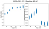 |
Fig. B.2. Amplitudes and Stokes V amplitudes for IF 3 in 0059+581 on the KP-SC baseline. This is an example of a baseline that has been flagged for times earlier than UTC 12 since the gain solution was judged to be unreliable. |
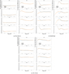 |
Fig. B.3. Smoothed R/L gain curves for three stations. Shown are the gain curves obtained for the original dataset (blue) and the curves obtained when the gain transfer techniques is only applied to datasets with the long baselines flagged. |
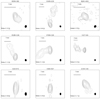 |
Fig. B.4. Same-level plotting comparison between CLEAN and DoG-HiT results: CLEAN. The conotour levels are [0.1%,0.2%,0.4%,...,51.2%] of the peak brightness emission. The convolution beam has been derived with uniform weighting and is shown in the lower left of the images. The scale of the image is shown in the top left with a bar of 3 mas in length. |
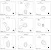 |
Fig. B.5. Same-level plotting comparison between CLEAN and DoG-HiT results: DoG-HiT. To allow for comparisons to the CLEAN images presented in Fig. B.4, the reconstructions have been blurred by the uniform weighting beam. |
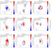 |
Fig. B.6. Calibration and imaging based on Homan et al. (2001). Illustrating the same parameters as in Fig. 4. |
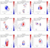 |
Fig. B.7. Calibration and Imaging with the gain-transfer technique, but the long baselines were flagged during the gain transfer. |
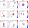 |
Fig. B.8. Results after a final self-calibration round at 15 GHz. Illustrating the same parameters as in Fig. 4. |
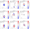 |
Fig. B.9. Results after a final self-calibration round at 23 GHz. Illustrating the same parameters as in Fig. A.2. |
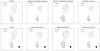 |
Fig. B.10. Reconstructions of 0149+218 with different assumptions, e.g., by CLEAN (left panel), with a LASSO scheme (CLEAN-like non-linear optimization) only fitting the closure quantities (second column), DoG-HiT fitting to amplitudes and closure quantities (third column) and DoG-HiT only fitting the closures (fourth row). |
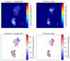 |
Fig. B.11. Polarized reconstructions of 0149+218 either using only the closure quantities for the reconstruction in total intensity (right column), or amplitudes and closures (left column). |
Appendix C: Impact of calibration methods on 1243−072 and 1546+027
Our approach for the calibration circular polarization has also been validated in App. B using an alternative gain estimation technique (running median rather than a smooth curve) and with an additional self-calibration step. For most sources, the relative structures remain consistent. Notably, in resolved double structures, the relative brightness varies. We observe two exceptions to a consistent result, namely, 1243−072 and 1546+027. That is, across all the tests conducted, the two sources, 1243 and 1546, consistently exhibited the most significant variations between methods. This strongly suggests that the circular polarization signal in these two sources may be influenced by the gain calibration process. In line with this, we have marked the estimates for these two sources in Tabs. 1 and 2 and have effectively excluded them from the broader interpretation. Upon inspecting the uv-coverage, this observation makes sense: 1243−072 and 1546+027 have the sparsest coverage and are the most weakly constrained sources in the dataset. Additionally, we would like to highlight an interesting aspect of this comparison. The recovered structure in 1243−072, when flagging long baselines, appears more similar to the reconstructions obtained using a running median than to those derived from our gain calibration approach. This may further indicate that our gain calibration method is more sensitive to the longer baselines than traditional techniques.
All Tables
All Figures
|
Fig. 1. Flowchart representing the similarities and differences between the pipeline presented in Homan et al. (2001, (left)) and our pipeline with DoG-HiT (right). Both pipelines illustrated here start post-calibration in AIPS. The data are processed in Difmap (pink), solved and adjusted for leakage terms in AIPS (yellow) and DoG-HiT in our pipeline, respectively (green), solved and applied for gain transfer, and finally imaged in full polarization. |
| In the text | |
|
Fig. 2. Final calibrated and flagged Stokes V amplitudes as a function of uv-distance (blue points) and the respective fit (red points). |
| In the text | |
|
Fig. 3. Reconstruction of data from 6–7 Jan. 2022 for nine target sources: 0059+581, 0149+218, 0241+622, 0528+134, 0748+126, 1127–145, 1243–072, 1546+027, and 2136+141. The figure shows maps for each source in linear polarization at 15 GHz (color coding: blue-low and red-high). The total intensity is indicated in white contours on each map. The contours are the [0.1%,0.2%,0.4%,…,25.6%,51.2%] levels of the peak brightness. The orientation of the linear electric vector position angle is plotted as white ticks, the total polarized intensity by the colormap. An individual convolution beam (natural weighting) is shown in the lower right corner of each map. The field of view is shown by the scale with 3 mas in the lower left. |
| In the text | |
|
Fig. 4. Circular polarization imaging results from 6–7 Jan. 2022 for nine target sources: 0059+581, 0149+218, 0241+622, 0528+134, 0748+126, 1127–145, 1243–072, 1546+027, and 2136+141. The figure shows maps for each source in circular polarization at 15 GHz (colorcoding: blue/red negative/positive). The total intensity is indicated in white contours on each map at levels of [0.1%,0.2%,0.4%,…,51.2%] of the peak brightness. An individual convolution beam is shown in the lower right corner of each map. The field of view and source size are shown by the scale, with 3 mas in the lower left. |
| In the text | |
|
Fig. 5. Reconstruction of data from 6–7 Jan. 2022 for the quasar 0528+134. The images show the resolved maps of: linear polarization at 15 GHz (color coding: blue-low and red-high) in the left panel. The total intensity is indicated in white contours. The linear electric vector position angle is plotted as white ticks. Right: circular polarization (colorcoding: blue-negative and red-positive). The total intensity is indicated in white contours. |
| In the text | |
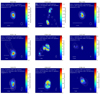 |
Fig. A.1. Same as Fig. 3, but at a 23 GHz observational frequency. |
| In the text | |
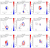 |
Fig. A.2. Same as Fig. 4, but at a 23 GHz observational frequency. |
| In the text | |
|
Fig. B.1. D-terms: CLEAN (diamond) vs. DoG-HiT (circle). Left panels show the right-handed solutions and the right panels the left-handed solutions. Solutions for various IFs are presented in various rows. |
| In the text | |
|
Fig. B.2. Amplitudes and Stokes V amplitudes for IF 3 in 0059+581 on the KP-SC baseline. This is an example of a baseline that has been flagged for times earlier than UTC 12 since the gain solution was judged to be unreliable. |
| In the text | |
|
Fig. B.3. Smoothed R/L gain curves for three stations. Shown are the gain curves obtained for the original dataset (blue) and the curves obtained when the gain transfer techniques is only applied to datasets with the long baselines flagged. |
| In the text | |
|
Fig. B.4. Same-level plotting comparison between CLEAN and DoG-HiT results: CLEAN. The conotour levels are [0.1%,0.2%,0.4%,...,51.2%] of the peak brightness emission. The convolution beam has been derived with uniform weighting and is shown in the lower left of the images. The scale of the image is shown in the top left with a bar of 3 mas in length. |
| In the text | |
|
Fig. B.5. Same-level plotting comparison between CLEAN and DoG-HiT results: DoG-HiT. To allow for comparisons to the CLEAN images presented in Fig. B.4, the reconstructions have been blurred by the uniform weighting beam. |
| In the text | |
|
Fig. B.6. Calibration and imaging based on Homan et al. (2001). Illustrating the same parameters as in Fig. 4. |
| In the text | |
|
Fig. B.7. Calibration and Imaging with the gain-transfer technique, but the long baselines were flagged during the gain transfer. |
| In the text | |
|
Fig. B.8. Results after a final self-calibration round at 15 GHz. Illustrating the same parameters as in Fig. 4. |
| In the text | |
|
Fig. B.9. Results after a final self-calibration round at 23 GHz. Illustrating the same parameters as in Fig. A.2. |
| In the text | |
|
Fig. B.10. Reconstructions of 0149+218 with different assumptions, e.g., by CLEAN (left panel), with a LASSO scheme (CLEAN-like non-linear optimization) only fitting the closure quantities (second column), DoG-HiT fitting to amplitudes and closure quantities (third column) and DoG-HiT only fitting the closures (fourth row). |
| In the text | |
|
Fig. B.11. Polarized reconstructions of 0149+218 either using only the closure quantities for the reconstruction in total intensity (right column), or amplitudes and closures (left column). |
| In the text | |
Current usage metrics show cumulative count of Article Views (full-text article views including HTML views, PDF and ePub downloads, according to the available data) and Abstracts Views on Vision4Press platform.
Data correspond to usage on the plateform after 2015. The current usage metrics is available 48-96 hours after online publication and is updated daily on week days.
Initial download of the metrics may take a while.