| Issue |
A&A
Volume 682, February 2024
|
|
|---|---|---|
| Article Number | A11 | |
| Number of page(s) | 23 | |
| Section | The Sun and the Heliosphere | |
| DOI | https://doi.org/10.1051/0004-6361/202347328 | |
| Published online | 26 January 2024 | |
Comparative clustering analysis of Ca II 854.2 nm spectral profiles from simulations and observations
1
Rosseland Centre for Solar Physics, University of Oslo,
PO Box 1029
Blindern,
0315
Oslo, Norway
e-mail: This email address is being protected from spambots. You need JavaScript enabled to view it.
2
Institute of Theoretical Astrophysics, University of Oslo,
PO Box 1029
Blindern,
0315
Oslo, Norway
3
Lockheed Martin Solar & Astrophysics Laboratory,
3251 Hanover St.,
Palo Alto, CA
94304, USA
4
Bay Area Environmental Research Institute,
NASA Research Park,
Moffett Field, CA
94035, USA
5
Institute for Solar Physics, Dept. of Astronomy, Stockholm University, AlbaNova University Centre,
10691
Stockholm, Sweden
Received:
30
June
2023
Accepted:
21
October
2023
Abstract
Context. Synthetic spectra from 3D models of the solar atmosphere have become increasingly successful at reproducing observations, but there are still some outstanding discrepancies for chromospheric spectral lines, such as Ca II and Mg II, particularly regarding the width of the line cores. It has been demonstrated that using sufficiently high spatial resolution in the simulations significantly diminishes the differences in width between the mean spectra in observations and simulations, but a detailed investigation into how this impacts subgroups of individual profiles is currently lacking.
Aims. We compare and contrast the typical shapes of synthetic Ca II 854.2 nm spectra found in Bifrost simulations having different magnetic activity with the spectral shapes found in a quiet-Sun observation from the Swedish 1-m Solar Telescope (SST).
Methods. We used clustering techniques to extract the typical Ca II 854.2 nm profile shapes synthesized from Bifrost simulations with varying amounts of magnetic activity. We degraded the synthetic profiles to observational conditions and repeated the clustering, and we compared our synthetic results with actual observations. Subsequently, we examined the atmospheric structures in our models for some select sets of clusters, with the intention of uncovering why they do or do not resemble actual observations.
Results. While the mean spectra for our high resolution simulations compare reasonably well with the observations, we find that there are considerable differences between the clusters of observed and synthetic intensity profiles, even after the synthetic profiles have been degraded to match observational conditions. The typical absorption profiles from the simulations are both narrower and display a steeper transition from the inner wings to the line core. Furthermore, even in our most quiescent simulation, we find a far larger fraction of profiles with local emission around the core, or other exotic profile shapes, than in the quiet-Sun observations. Looking into the atmospheric structure for a selected set of synthetic clusters, we find distinct differences in the temperature stratification for the clusters most and least similar to the observations. The narrow and steep profiles are associated with either weak gradients in temperature or temperatures rising to a local maximum in the line wing forming region before sinking to a minimum in the line core forming region. The profiles that display less steep transitions show extended temperature gradients that are steeper in the range−3 ≲ log τ5000 ≲ −1.
Key words: Sun: atmosphere / Sun: chromosphere / techniques: spectroscopic / line: formation
© The Authors 2024
 Open Access article, published by EDP Sciences, under the terms of the Creative Commons Attribution License (https://creativecommons.org/licenses/by/4.0), which permits unrestricted use, distribution, and reproduction in any medium, provided the original work is properly cited.
This article is published in open access under the Subscribe to Open model. This email address is being protected from spambots. You need JavaScript enabled to view it. to support open access publication.
1 Introduction
Thanks to advances in instrumentation, it is now possible to routinely obtain spatially resolved spectra from the solar surface at spatial resolutions of tenths of arcseconds or even finer. These detailed spectra contain a wealth of information. For lines formed in the dynamic solar chromosphere, spectral shapes become increasingly complex, especially as the spatial resolution increases. To extract the maximum information from observations, it is crucial to understand how different spectral lines are formed in a dynamic atmosphere. Three-dimensional, radiative magnetohydrodynamic (3D rMHD) simulations of the solar atmosphere (e.g., Stein & Nordlund 1998; Vögler et al. 2004; Gudiksen et al. 2011; Iijima & Yokoyama 2015; Khomenko et al. 2018; Przybylski et al. 2022; Hansteen et al. 2023) have become a powerful tool to help interpret spectral observations and learn how spectral lines form.
For the solar photosphere, the self-consistent treatment of convection in 3D simulations can reproduce the (mean) shapes of spectral lines in great detail (e.g., Asplund et al. 2000), and also leads to a mean temperature stratification that agrees very well with a wealth of observational diagnostics (Pereira et al. 2013a). However, the solar chromosphere is a much more demanding problem, and current simulations do not yet reproduce the variations in chromospheric lines as well as they do for photospheric lines. For example, synthetic profiles of chromo-spheric lines tend to be narrower than observed (Leenaarts et al. 2009) and can show weaker emission (Leenaarts et al. 2013b; Rathore et al. 2015a). Although they cannot yet reproduce all chromospheric line shapes, 3D rMHD simulations have been instrumental in forward-modeling studies that shape our understanding of most spatially resolved line formation, for example from the formation of the Hα line (Leenaarts et al. 2012) and the Ca II H&K lines (Bjørgen et al. 2018). Such studies are also very important in the development of, and interpretation of, data from new observatories, as shown by the MUSE mission (De Pontieu et al. 2022; Cheung et al. 2022) and by the IRIS mission (De Pontieu et al. 2014), for which a series of papers (Leenaarts et al. 2013a,b; Pereira et al. 2013b, 2015; Rathore & Carlsson 2015; Rathore et al. 2015a,b; Lin & Carlsson 2015; Lin et al. 2017) provides unique insight into the formation of UV lines.
Most forward-modeling studies follow a well-tested pattern of first synthesizing spectra from 3D rMHD simulations, using either fully 3D radiative transfer or the 1.5D approximation where each simulation column is treated as an independent plane parallel atmosphere, and then comparing spectral signatures with the thermodynamical conditions of the underlying atmosphere. Given the sheer number of individual spectra (typically on the order of millions for one simulation), it is not possible to study each spectrum in detail. To date, most studies have focused on either the properties of spatially averaged spectra or on the distributions of simple spectral properties (e.g., line shifts, line widths, position and amplitude of emission peaks). The main goal of this work is to extend previous approaches and use more information from the line profiles by means of clustering techniques.
In a previous paper (Moe et al. 2023, hereafter Paper I), we discuss and demonstrate the use of clustering techniques, such as k-means (Steinhaus 1956; MacQueen 1967) and k-Shape (Paparrizos & Gravano 2015) in a forward-modeling context. Through the use of k-means and k-Shape clustering, we investigated the variety of Ca II 854.2 nm spectral shapes present in a 3D rMHD simulation, and how those shapes correlated with the structure of the atmospheric columns they arose from. Here, we want to extend this approach to different types of atmospheres and observations. Again, we restrict the analysis to the Ca II 854.2 nm line, which is a widely observed diagnostic of the chromosphere (e.g., Cauzzi et al. 2008; Chae et al. 2013; de la Cruz Rodríguez et al. 2015a; Quintero Noda et al. 2016; Kuridze et al. 2017; Molnar et al. 2021).
In this work we investigate the typical shapes of Ca II 854.2 nm line profiles, and what they tell us about the solar atmosphere. We study how profile shapes vary across simulations with different amounts of magnetic field. In addition, we make a critical comparison between the synthetic and observed clusters of line profiles. With access to the full thermodynamical state of the underlying simulated atmospheres, we investigate how different clusters of atmospheres are structured, and how different quantities influence the formation of the Ca II 854.2 nm line.
This paper is organized as follows. In Sect. 2 we describe the simulations, spectral synthesis, observations, and clustering methods used. In Sect. 3 we describe the results from the spectral clustering, look in detail at typical families of spectra, and compare simulations with observations. We discuss our results in Sect. 4, and finish with our conclusions in Sect. 5.
2 Methods
2.1 Simulations
We made use of three distinct 3D rMHD simulations run with the Bifrost code (Gudiksen et al. 2011). The goal was not to reproduce the observed region exactly, but to experiment with different amounts of magnetic activity. It should be noted that none of these simulations accounts for the nonequilibrium ionization of hydrogen.
The first simulation, hereafter ch012023, is magnetically quiet and has a field configuration resembling a coronal hole. It is the same simulation used in Paper I, and is described in more detail by Moe et al. (2022). Its box size is 12 × 12 Mm2 horizontally (with 23 km horizontal grid size) and 12.5 Mm vertically, and its mean unsigned magnetic field at z = 0 is 3.7 mT (37 G). The vertical grid is nonuniform, and is spread over 512 points.
The second simulation, hereafter nw012023, has the same physical extent and horizontal spatial resolution of ch012023, but a different magnetic field configuration. Here a stronger magnetic field has been injected into the middle of the box, separating the regions of opposite magnetic polarity. Its mean unsigned magnetic field at z = 0 is 8.6 mT (86 G). The vertical grid spans 16.8 Mm with 824 nonuniformly distributed grid points.
The third simulation, hereafter nw072100, is very different from the other two. It has a much larger spatial extent, 72 × 72 Mm2 horizontally and nearly 60 Mm in the vertical direction. The vertical grid spans 1116 nonuniformly grid points. Hansteen et al. (2023) describe this simulation in detail. It has regions with a much stronger magnetic field, and is included in this study as a more extreme case. It is not meant to reproduce the quiet observations we describe below, but instead as a case study for line profiles in a more active atmosphere. Its spatial resolution, with a horizontal grid size of 100 km, is also coarser than the other two models. As Hansteen et al. (2023) note, the numerical resolution can also affect the mean spectral properties, such as the width, so one should keep that in mind when comparing nw072100 with the other simulations.
We note that throughout this paper we define the positive vertical axis to be pointing outward (i.e., positive vertical velocities correspond to upflows).
2.2 Synthesizing profiles
As in Paper I, for the present paper we used the fully 3D radiative transfer code Multi3D (Leenaarts & Carlsson 2009), with the polarization-capable extension (Calvo & Leenaarts in prep.), to generate synthetic spectra of the Ca II 854.2 nm line. Although we focus our analysis on the shapes of the intensity profiles, Stokes I, we computed full Stokes profiles accounting for the Zeeman effect under the field-free approximation (i.e., polarization is accounted for in the final formal solution, using atomic populations iterated to convergence considering only the intensity). Multi3D solves the non-local thermodynamical equilibrium (NLTE) radiative transfer problem considering one atomic species at a time (i.e., it does not simultaneously solve for multiple species). Here we used a model Ca atom that consists of six levels (five bound levels and one continuum level). As 3D radiative transfer is computationally expensive, we trimmed away the deeper and higher parts of the snapshots, which should have a negligible influence on the emergent spectra, in order to speed up the computations. We cut the top a few grid points above the horizontal plane where all simulation columns had exceeded 50 kK, and we cut the bottom below the horizontal plane where the granulation pattern was no longer discernible in maps of the temperature. This cutting reduces ch012023 to 410 vertical grid points between 8.0 Mm and −0.42 Mm, nw012023 to 552 vertical grid points between 6.8 Mm and −1.0 Mm, and nw072100 to 720 vertical grid points between 29 Mm and −1.3 Mm. All spectra were computed with the assumption of complete redistribution (CRD), which is a reasonable choice for this line (Uitenbroek 1989; Bjørgen et al. 2018), and we did not account for iso-topic splitting, which has some influence on the line shapes (Leenaarts et al. 2014). Furthermore, statistical equilibrium (SE) was assumed, as nonequilibrium ionization of Ca is unimportant for the formation of the 854.2 nm line (Wedemeyer-Böhm & Carlsson 2011).
Our analysis in this paper is focused on the spectral range λ0 ± 0.1 nm, where λ0 is the central wavelength of the Ca II 854.2 nm line. This range encompasses the chromospheric line core, as well as parts of the photospheric wings. In terms of formation heights, we find, for all our simulations, that the line core reaches unity optical depth at around log τ5000 ≈ −5.3 on average, where τ5000 is the optical depth for light at 500 nm (5000 Å), while the farthest parts of the wings in this spectral range reach unity optical depth at log τ5000 ≈ −1.2 on average. The formation height initially increases slowly from the far wings toward the line core, until the transition point from wing to core is reached (at about log τ5000 ≈ −2); from there the formation height rapidly increases toward the maximum at the line core. This is in reasonable agreement with the study by Quintero Noda et al. (2016), which looked at the response functions for the Ca II 854.2 nm line in the semi-empirical FALC atmosphere (Fontenla et al. 1993).
2.3 Observations
The observations were acquired with the CRISP instrument (Scharmer et al. 2008) at the Swedish 1-m Solar Telescope (SST; Scharmer et al. 2003). CRISP is a Fabry-Pérot tunable filtergraph that is capable of fast wavelength switching and imaging at high spatial resolution. We observed an area near the edge of an equatorial coronal hole close to disk center at (x,y) ≈ (−119″, −106″) on 24 June 2014. The heliocentric viewing angle was µ ≈ 0.99. CRISP was running a program observing the Hα and Ca II 854.2 nm lines in spectral imaging mode plus single wavelength Fe I 630.2 nm spectropolarimetry to produce magne-tograms based on Stokes V of the line wing. Here we concentrate on the Ca II 854.2 nm data, which consist of spectral line scans at 25 wavelength positions between ±0.12 nm with 0.01 nm steps. The full time series started at 08:27:14 UT has a duration of 01:15:37 and a temporal cadence of 11.5 s (the time it takes to sample the same wavelength again). The data were processed using the CRISPRED data reduction pipeline (de la Cruz Rodríguez et al. 2015b), which includes multi-object multi-frame blind deconvolution (MOMFBD; van Noort et al. 2005) image restoration. The seeing conditions were excellent and with the aid of the adaptive optics system and MOMFBD image restoration, the spatial resolution was close to the diffraction limit of the telescope for a large fraction of the time series (λ/D = 0″. 18 at the wavelength of Ca II 854.2 nm for the D = 0.97 m clear aperture of the SST). For most of our analysis we use a single time step with particularly good seeing conditions, when the Fried’s parameter r0 for the ground-layer seeing was measured to be above 40 cm. The field of view was cropped to about 50″ × 50″ and the plate scale is 0″.057 pixel−1. In Fig. 1 we show an overview of the field of view used for the spectral clustering, including the 854.2 nm line core intensity and a magnetogram from the Stokes V of the Fe I 630.2 nm line.
2.4 Degrading the synthetic profiles
In order to fairly compare the simulations to the observations, we needed to degrade them spectrally and spatially, as well as resample them. This is done in a four-step process. First, the synthetic spectra are convolved with a Gaussian in the spectral domain, using the 10.5 pm full width at half maximum (FWHM) spectral instrumental profile of CRISP. Second, the spectra are downsampled in the spectral domain to match the 21 wavelength points of the narrowband filter, ranging from λ0 ± 0.1 nm, where λ0 is the central wavelength of the Ca II 854.2 nm line. Third, the spectra are convolved in the spatial domain with a 2D Gaussian with a 0″.18 FWHM to match the telescope’s resolution. Finally, the synthetic spectra are interpolated and resampled to match the 0″.057 pixel−1 plate scale. We note that the synthetic profiles are computed for a disk-center viewing angle (i.e., for µ = 1) and we do not project them to the µ ≈ 0.99 viewing angle of the observations because the difference in viewing angle is so minor.
An additional difference between the synthetic and observed spectra is that the synthetic spectra are an instant snapshot of the atmosphere at a given time, while CRISP observations have a given exposure time and scan time (not all wavelengths are observed at the same time), during which time the atmosphere can change. As Schlichenmaier et al. (2023) show, this should be accounted for in order to do the most accurate comparisons between synthetic and real observables. We did not perform an accurate time-averaged comparison because of several factors: first, the simulation snapshots are typically not saved at such high cadence; second, 3D NLTE radiative transfer is computationally very expensive; and finally, because the time to acquire each of our CRISP scans is already short (less than 10 s), we did not expect the observed profiles to differ significantly from an “instant” snapshot.
In most of our analysis we use the original, nondegraded synthetic profiles. This is especially relevant when comparing synthetic profiles and atmospheric quantities since the simulations are not degraded. However, the degraded profiles are an important check when making a direct comparison with observations, and also to make sure that the overall range of synthetic spectral clusters is not significantly changed by the observational conditions.
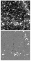 |
Fig. 1 Overview of the observed region. The images show the field of view used for the spectral clustering, at 2023-06-24T09:15. Top: Ca II 854.2 nm line core intensity. Bottom: Fe I 630.2 nm line wing Stokes V, a proxy for magnetic field. |
2.5 Clustering methods
We employ the k-means and k-Shape (Paparrizos & Gravano 2015) clustering methods on both synthetic and observed intensity profiles for the Ca II 854.2 nm line core. A thorough description for how these methods work, and how their results compare, can be found in Paper I. In short, they both iteratively partition a set of profiles among a predefined number of k clusters, grouping the profiles together based on some metric of similarity. For k-means that metric is the Euclidean distance, while k-Shape uses a more shape-based distance measure and also compares the profiles for a range of relative wavelength shifts. The k-Shape method assumes z-normalization (i.e., that each profile is scaled to have zero mean and unity variance). In practical terms, k-Shape is independent of the profiles’ amplitudes and largely independent of the profiles’ Doppler shifts, and it does, at least in some cases, do better at distinguishing profile shapes than k-means. It is, however, considerably slower computationally, and the amplitude invariance can group together profiles of rather different intensities. We used it here as a complementary tool to k-means, to check whether it generates clusters containing profile prototypes not seen in our k-means experiments.
We used the same libraries (scikit-learn, Pedregosa et al. 2011; tslearn, Tavenard et al. 2020) and methods (k-means++ initialization, Arthur & Vassilvitskii 2007, for the k-means method) as before. Some simple modifications of the tslearn library were implemented to make k-Shape run in parallel.
We performed the clustering not on the full line profile, but only in the central part within λ0 ± 0.1 nm, where λ0 is the central wavelength of the Ca II 854.2 nm line. We made this choice for two reasons: this central region is the part formed in the chromosphere (already at 0.1 nm the line probes reversed granulation), and because our observations were limited to λ0 ± 0.12 nm. In the rest of this work, when we refer to continuum we mean the local continuum at 0.1 nm, not the real continuum in the far wings. In order to give equal weight to all parts of the line profile, we interpolate our synthetic spectra to an equidistant grid of wavelength points in the range λ0 ± 0.1 nm. The degraded synthetic spectra and the observations are given on the same equidistant grid of 21 wavelength points in the same range.
3 Results
3.1 Overview
We used the k-means clustering method with k = 100 clusters and ten re-initializations for the Stokes I profiles belonging to one snapshot for each of our simulations (to both degraded and nondegraded spectra) and to the observations. This particular choice of k was made after experimentation as a trade-off between accuracy in the clustering and human readability of the results. All cluster results shown in this manuscript stem from performing the clustering on the Stokes I profiles without any normalization. For the synthetic profiles, the intensity units were nWm−2 Hz sr−1, and for the observations the intensities were not absolutely calibrated, so we used the arbitrary data number (DN) from the reduction. Additionally, we also performed both k-means and k-Shape clustering on the z-normalized intensity profiles to test whether any clusters with shapes not seen in the nonnormalized spectra would be revealed.
In an effort to provide some quantitative measures of the profile shapes in the following discussion, we define the depth of a profile as the difference between the maximum and minimum intensity in our considered wavelength window of λ0 ± 0.1 nm. We also quantify the line widths by defining the FWHM as the width between the points having intensities half-way between the minimum and maximum intensity in this wavelength window. We used these measures only on the mean profiles in clusters showing simple behavior, since they do not work well for more complicated line shapes.
3.2 Spatially averaged profiles
Before moving to the clustering analysis we look at the spatially averaged spectra. In Fig. 2 we plot the mean spectra, plus the 1σ variations around the mean for the observations and the three simulations. To allow a direct comparison, the synthetic spectra were degraded to the observational conditions before computing the mean and 1σ variations, and all spectra were normalized by the local continuum at λ0 + 0.1 nm.
A noteworthy difference is that the simulations, even after spatial and spectral degradation, have spatial variations that are about twice as large as the variations in the observations. In addition, the amount of variation does not seem to change much from the quieter ch012023 to the more active nw072100. The nw012023 mean profile is redshifted because the particular snapshot we used has a net downflowing atmosphere, leading to a shifted and more asymmetric mean profile. In terms of line width, the observations are broader than all simulations, but both ch012023 and nw012023, which have a horizontal grid size of 23 km, are much closer to the observations than nw072100, which has a grid size of 100 km. In numbers, the FWHMs of these mean profiles are 66 pm, 55 pm, 49 pm, and 31 pm, respectively, for the observations, ch012023, nw012023, and nw072100. Without spectral and spatial degradation, we obtained FWHMs of 53 pm, 48 pm, and 25 pm, respectively, for the mean profiles from ch012023, nw012023, and nw072100. We note that when we discuss the FWHMs of the synthetic profiles in the following sections, we refer to the undegraded profiles at native spatial and spectral resolution.
3.3 Stokes I clusters
3.3.1 Observations
We show the resulting clustering for our observations in Fig. 3. This clustering was performed for a single CRISP scan (about 106 spectra in total). We also experimented with scans taken at different times, and clustering multiple scans at the same time, but find little variation in the results. The most frequent types of clusters hardly change, and the few differences are mostly in the least frequent clusters, which can vary slightly from scan to scan. Hereafter we discuss only the observations shown in Fig. 3 since they were taken with some of the best conditions and we find them representative of the general properties of the observed region.
For the most part, the observed spectra appear quite tightly constrained, with little variation inside most clusters and typical line shapes not too dissimilar between clusters. The majority of clusters present absorption profiles with fairly wide line cores and gently curving transitions from the inner wings to the core; prime examples are #10 and #44. Most of the variation for these profile types comes as gentle Doppler shifts of the line, sometimes accompanied by a slight asymmetry (e.g., #46 and #87) or a larger asymmetry (e.g., #85). There is also some variation in the width of the profiles, and how steep the transitions from the wings to the core are (compare, e.g., #30 with #91). Additionally, there is some variation in local continuum and line depth (contrast, e.g., #98 and #62). On the whole, however, the general shapes are similar.
On the other hand, there are some “families” of clusters that break the mold. One distinct type is the very shallow, sometimes almost triangular, profiles of clusters, such as #45, #60, #63, #66, #81, #84, and #90. Some of these clusters include profiles similar to the “raised core” profiles found by de la Cruz Rodríguez et al. (2013), although the magnetic configuration of our observations is somewhat different from theirs: ours has a smaller magnetic canopy. There is also cluster #99 which displays emission on the left side of the core, similar to the chromospheric bright grain-like (CBG-like) profiles we studied in Paper I. This is the only cluster that shows very clear emission, but there are a few cases (#77, #79, #80, #88, #89) where there are some cluster members that show enhanced intensities around the “elbow” marking the transition from wings to core. Beyond those, there are the three clusters (#93, #97, and particularly #100) that are somewhat less constrained than the others, and display more complex shapes.
As mentioned previously, we also used the k-Shape method alongside k-means to cluster these profiles after applying z-normalization. The purpose of this is to ensure that we get a more complete view of which profile shapes are present in our data. These experiments yielded results that are qualitatively very similar to the unnormalized case, the largest difference being that they picked up and separated out a few clusters showing flat-bottomed or complex line cores which mostly belong to clusters, such as #63, #81, #90, #97, and #100 in Fig. 3. That is not surprising as the z-normalization amplifies the relative differences in amplitude between the members of the shallow clusters, making their shapes more distinct. As for the profiles in #100, z-normalization reduced the difference in absolute intensity between members of that cluster and the other clusters, so that the different shapes present in that cluster could be separated and put into other clusters more based on shape than amplitude. For our purposes in this paper, we are interested in both the profile shapes and their absolute amplitudes, so we focus on the clusters with unnormalized profiles; however, we would like to emphasize that there is some diversity in the shapes found for the least constrained clusters.
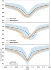 |
Fig. 2 Mean spectra with 1σ variations for observations and three simulations. The shaded bands show, for each wavelength, the 1σ range of departures from the mean. All spectra were normalized to the local continuum at λ0 + 0.1 nm. The synthetic spectra were degraded to match the conditions of the observations. |
3.3.2 ch012023 clusters
We now turn to the clusters retrieved from our synthetic observations. We carried out the clustering for the original and degraded synthetic spectra. We find the same general trends for the retrieved clusters in both cases, with the main difference being reduced variations in each cluster, and a reduced range in the continuum variations (as expected from the spatial degradation) in the clusters of degraded spectra. Since we look into the atmospheric structures for some of the synthetic clusters below, here we focus our analysis on the undegraded profiles as the spatial and spectral degradation makes it difficult to assign unequivocal values of the atmospheric parameters to the degraded spectra. We show the ch012023 clustering results for the original resolution in Fig. 4, while a similar figure for the degraded cases is shown in Appendix A.
The ch012023 simulation represents a quiet-Sun scene, with magnetic fields resembling the conditions of a coronal hole. Thus, it is noteworthy that in Fig. 4 so many clusters show profiles with emission features and strong asymmetries. This is an important difference from the clusters found in the observations, which contain mostly absorption profiles. Among the ch012023 clusters we find CBG-like profiles (e.g., #61, #70, #71, #89, #93, #94) and the double-peaked profiles (seen in #41, #81, #99) discussed in Paper I, to the complicated and poorly constrained clusters, such as #30, #36, and #60. Furthermore, cluster #100 displays reversed CBG-like profiles (specifically, the emission is on the red side of the core) that are not clearly visible in the observations. Beyond that, we have cases of enhanced elbows (e.g., #63, #77, #78), where there is emission around either the blue, the red, or both transitions from wings to core; these features are only weakly seen in the observed clusters. We also find sharply asymmetric absorption profiles (e.g., #22, #87, #95) and flat-bottomed profiles (e.g., #45, #67) that do not match the clusters in the observations.
Not only are the shapes found more varied and the number of clusters with exotic shapes larger, but the number of profiles belonging to these atypical clusters is far larger in the simulation than in the observations. As an example, just the three clusters #61, #70, and #71 in Fig. 4 contain a greater percentage of profiles (roughly 1.7 vs. 1.4% of all profiles), than all the observed clusters with clear emission features (#77, #79, #80, #88, #89, #99 in Fig. 3).
There are profiles that appear similar between the observations and simulations as well. We find several more typical absorption profiles (e.g., #23, #34, #51, #80, #84) and some of the shallower profiles, such as #4 and #8 in Fig. 4, bear a strong resemblance to their observed counterparts, such as #63 and #81 in Fig. 3. However, there are some marked differences between the typical absorption profiles found in the observations versus the simulation. The most noticeable difference is the width of the profiles as the synthetic profiles are narrower than the observed profiles. There are, however, variations in how large this difference is; the wider profiles in Fig. 4, for example #34 and #51 (FWHM of 47 pm and 40 pm, respectively) are not that much narrower than #58, #69, #83, or #91 in Fig. 3 (FWHM of 50 pm, 50 pm, 48 pm, and 49 pm, respectively). On the other hand, the narrow synthetic profiles, such as #32, #57, #69, or #75 in Fig. 4 (FWHM of 29 pm, 25 pm, 27 pm, and 26 pm, respectively), contrast greatly with the observational clusters.
Another difference is the shape of the transition from wings to core; the synthetic profiles generally have a much steeper transition, in some cases almost cliff-like, than the observed profiles, which tend to exhibit far smoother and more gently curving slopes. This difference is particularly noticeable for narrow profiles, such as #69, but it also occurs for wider profiles, such as #84. More similar to the observations, in terms of shape, are the profile clusters #9, #14, and #23 in Fig. 4, which compare quite well with #43, #48, #57, and #77 in the observation clusters shown in Fig. 3. In sum, we find large differences between the clusters obtained from our observation and from our quietest simulation, though there are some instances were there are strong resemblances between them.
As with the observed spectra, we have also performed k-Shape and k-means clustering using z-normalization on these spectra and on the other synthetic spectra. Similarly to the observational case, but even more pronounced, we find several clusters with rather complicated line core shapes, which correspond to the least constrained or shallowest clusters for the unnormalized intensities. These complicated line core shapes include flat-bottomed cores, W-shaped central reversals, and M-shaped double-peaked central reversals that both do and do not exceed the intensities of the nearby inner wings. Again, a longer discussion about the varieties of shapes revealed when ignoring the absolute intensities is beyond the scope of the current work, but we would like to note that there are complicated spectral profiles found in the least constrained clusters, such as # 0, #55, #7 , and #99, and also in the seemingly simple shallow shapes, such as #3, #4, #11, and #18 (see Fig. 4). In Appendix A we briefly discuss and show the clustering results obtained with k-Shape on the z-normalized profiles for the observation and the ch012023 simulaiton. While we have not studied the z-normalized clustering results for the other simulations’ synthetic spectra in detail, at first impression they seem to display the same tendencies as in this case.
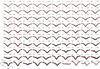 |
Fig. 3 k-means clusters of Ca II 854.2 nm observed spectra, using 100 clusters, sorted from most to least frequent. The red line denotes the average of all line profiles belonging to each cluster (thin black lines). The fraction of all profiles belonging to each cluster is indicated as a percentage next to the cluster number. The gray line indicates the position of λ0, the rest wavelength. |
 |
Fig. 4 k-means clusters of Ca II 854.2 nm synthetic spectra from the ch012023 simulation. The legend is the same as in Fig.3. |
3.3.3 nw012023 clusters
In Fig. 5 we show the results of applying the same type of clustering to the more magnetically active simulation nw012023. On the whole, the results are quite similar to what we previously saw for the quiet ch012023 simulation, with all the same shapes found in one being mirrored in the other. The primary difference in the clustering results for the nw012023 simulation compared to the ch012023 simulation is that the intensity values span a wider range; that is, some profiles are deeper, and emission peaks can also reach higher. Some of the clusters also seem to display more variance, meaning the cluster centroids seem to be less representative of the individual cluster members and there is likely quite a bit of mixing between different shapes in those clusters (e.g., #9, #36, #61, #74 in Fig. 5). Similar poorly constrained clusters were also seen for the ch012023 simulation (e.g., #73 and #93 in Fig. 4), but here they seem to be even stronger.
As can be seen in Appendix A, the effect of spatial and spectral degradation is a major decrease in within-cluster variance, but the key differences to the observation clusters remain.
3.3.4 nw072100 clusters
Finally, we show the clustering results for the nw072100 simulation in Fig. 6. In this case we still see more extreme shapes than in the other two simulations, but many of the cluster shapes are similar. The variance within clusters appears to be significantly larger than before (e.g., #24, #69, #92). The profile amplitudes are also generally larger; that is to say, many of the emission features have higher peak intensities and several of the absorption profiles are deeper. This is as expected since this simulation is more active and vigorous than the other two. There is one new family of clusters that appears for this simulation, namely the very broad emission profiles in clusters #93, #94, and #96. These profiles appear to have somewhat similar shapes, but much broader, to the CBG-like profiles seen in both the previous cluster results and in other clusters for this simulation (e.g., #74, #84, #89). However, looking into their atmospheric structure (plotted in Fig. B.1) we find that #93, #94, and #96 are associated with high temperatures (≳7 kK) and fast downflows (≪−8 km s−1) in the range −6 ≤ log τ5000 ≤ −4, where τ5000 is the optical depth for light at 500 nm (5000 Å), and show strong (>10 mT in absolute value) vertical magnetic field components over most of the line forming region.
In terms of the profile widths for the more typical absorption profiles, they are narrower in this simulation compared to the other two simulations; the narrowest profile clusters in Fig. 6 (e.g., #55, #71, #88 with, respectively, FWHMs of 22pm, 19 pm, 19 pm) are clearly less wide than any of the clusters we see in Figs. 4 or 5. However, there are also several clusters showing quite wide absorption profiles (e.g., #52, #61, #95 in Fig. 6, with FWHMs of, respectively, 42 pm, 36 pm, 44 pm) that seem comparable with the moderately wide clusters for the two higher resolution simulations. The typical absorption profiles are narrower in nw072100, which has the lowest spatial resolution, which is consistent with the findings of Hansteen et al. (2023).
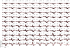 |
Fig. 5 k-means clusters of Ca II 854.2 nm synthetic spectra from the nw012023 simulation. The legend is the same as in Fig. 3. |
3.4 Atmospheric structure for selected clusters
So far the clustering results have shown us how similar, and dissimilar, the profiles are among the simulations and compared to the observation. We now take a detailed look at the atmospheric structure for a few selected clusters of synthetic profiles in order to see which trends in the atmospheric parameters correlate with these cluster families. We focus on four families of clusters, whose mean profiles are all in absorption. The first family is composed of wide profiles: profile shapes that show a broad line core, and typically stronger continuum intensities. The second is composed of narrow profiles: clusters that have some of the narrowest line widths. The third is composed of shallow profiles: lines with the smallest difference between wing and core intensity. The fourth family is composed of clusters of line profiles that have the gentlest transition (i.e., the most gradual) from line wings to line core. For each of these families, we selected four representative clusters from each of the simulations.
We elect to look at the widest and the narrowest profiles because the line width is one of the more obvious discrepancies between the simulations and observations, and it is therefore interesting to see which type of atmospheric structures can gives rise to narrow and broad lines. This might in turn provide indications to what our simulations are lacking compared to the real sun. For the other two families, the shallow and the gently curving clusters, we chose to investigate them because they are very reminiscent of clusters from the observations (e.g., cluster #81 in Fig. 3 appears quite similar to #4 in Fig. 4), and thus their atmospheric structures likely resemble more closely conditions in parts of the solar atmosphere.
The clusters for each family were manually selected as it is somewhat difficult to formulate quantitative criteria for whether a cluster belongs in one family or another. As such, there is some subjectivity involved in our particular choice of clusters for detailed analysis. That is why we look at several examples for each cluster type and simulation; we intend to discover the qualitative trends in atmospheric structure for the cluster families without relying on single examples.
Furthermore, it is important to recognize that there can be quite wide variations within clusters, and that even though the cluster means may appear “well behaved,” they are not necessarily fully representative of the individual profiles that make up the clusters. Therefore, the way we investigated these clusters is by carefully examining plots like that in Fig. 7; the figure displays the atmospheric structure for each profile in the clusters #80, #84, #57, #75 from Fig. 4, which are, respectively, two of the wider and two of the narrower clusters found for ch012023. The individual profiles making up the clusters are stacked along the vertical axis; the number indicated is the profile number. The leftmost columns show the Stokes I and Stokes V profiles, normalized to the nearby continuum at approximately λ0 + 0.95 nm, as a function of wavelength. The three rightmost columns show the stratification of temperature, line-of-sight velocity, and line-of-sight magnetic field strength against log τ5000. These plots show the individual variations within the clusters, and make clearer the less common atmospheric features, which are not as easily seen when considering averages. As an example of this, some of the narrow profiles have enhanced temperatures stretching across the whole range −5 < log τ5000 < −2 that correlate with emission in the transition from line wings to line core. For the sake of brevity, we show in Fig. 7 only a few representative clusters in detail. For the remaining selected clusters in each group, we show only a summarized view as in Fig. 8. However, we analyzed each of the selected clusters in detail. To aid in the comparison of the clusters across both type and family, we provide an overview of the estimated line widths and depths for mean profiles of selected clusters in Tables 1–3.
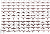 |
Fig. 6 k-means clusters of Ca II 854.2 nm synthetic spectra from the nw072100 simulation. The legend is the same as in Fig. 3. |
3.4.1 Wide profiles
In Fig. 8 we show the spectra and atmospheric quantities averaged over four different clusters of each simulation, along with the mean spectrum and atmospheric quantities averaged over the full simulation box. The averaging of the atmospheric quantities was performed over τ5000 isosurfaces. The clusters we selected correspond in Fig. 8 to clusters with wide line profiles, and their numbers are #34, #51, #80, #84 from ch012023 (Fig. 4); clusters #5, #17, #88, #97 from nw012023 (Fig. 5); and clusters #52, #61, #70, #95 from nw072100 (Fig. 6).
For the ch012023 case there appears to be a common trend for the wider clusters in terms of temperature, vertical velocity, and vertical magnetic field strength. The temperature goes from a moderately hot bottom to a cold layer that extends to the end of the line forming region, where log τ5000 is approximately between −5.5 and −5. The velocities are mostly weak or moderate (absolute values of <2.5 km s−1), as are the vertical magnetic field strengths (absolute values of <5 mT). A slight exception to the general tendencies are the profiles around profile number 200 of cluster #84, seen in the second row of Fig. 7. They show a noticeable widening on the blue side, and here the atmospheric structure shows a region of high temperatures extending below log τ5000 = −5 coinciding with a moderately strong upflow (υz ~ 3 km s−1).
For the nw012023 case, we find that there are two general types of atmospheres that produce the wide clusters. The first type, #5 and #17 from Fig. 5 go from temperatures close to the simulation’s mean temperature at the bottom, via a fairly constant gradient, to extended cold layers around log τ5000 ≈ −5 and below. The atmospheres of these profiles have weak to moderate vertical velocities of the downflowing variety (υz > −5 km s−1), along with weak to moderate magnetic field strengths of either polarity (absolute values of <5 mT), throughout the line forming region. The other type, #88 and #97 from Fig. 5, start with hotter bottom layers where the temperature does not decrease much before log τ5000 ≈ −3, or sometimes not even before log τ5000 ≈ −5. These wide profiles with enhanced temperatures correlate with moderate to strong downflowing velocities (υz < −5 km s−1) reaching up to log τ5000 ≈ −5, at which point strong upflows (υz > 5 km s−1) appear. They also coincide with strong magnetic fields of both polarities (absolute values of > 10 mT), which however taper off around log τ5000 ≈ −5. The hotter lower atmospheres in these types of profiles also help explain why the local continuum is much higher, and since the temperature gradient is shallow until log τ5000 ≈ −3, and only then becomes steep, the transition from continuum to line core in the profile is more abrupt, in contrast with clusters #5 and #17 whose mean profiles have a smoother transition from wing to core.
For the nw072100 case, the trend across all four clusters is that they start at higher than average temperatures at the bottom and decrease to a minimum around log τ5000 ≈ −4.5. The vertical velocities are mostly weak (<2.5 km s−1) up to log τ5000 ≈ −5, except for the hottest cluster with the shallowest temperature gradient (#95 in Fig. 6), which has many moderately strong downflows (υz ≤ −2.5 km s−1) throughout the line forming region. This is also the cluster with the strongest vertical magnetic field strengths (absolute values of >10 mT), although the other clusters also have some moderately strong fields present. In all clusters both magnetic polarities appear throughout the atmospheric columns.
In summary, similarities across these clusters of wide profiles are seen in the temperature structures, and in part in the velocities. All the clusters show a negative temperature gradient with height, with different slopes for different clusters, and at log τ5000 ≈ −1 they have above average temperatures. The hottest atmospheres, with the weakest temperature gradients, are correlated with the strongest vertical velocities and vertical magnetic field strengths. On the other hand, the colder atmospheres tend to have weak velocities and field strengths throughout the considered regions. A significant finding is that some of the widest synthetic profiles occur in the absence of significant vertical velocities.
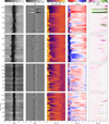 |
Fig. 7 Individual spectra and atmospheric structure of selected clusters from the ch0l2023 simulation. From left to right, the first two columns show the Stokes I and V (normalized to the nearby continuum, around λ0 + 0.95 nm), while the last three columns show the temperature, vertical velocity, and vertical magnetic field as a function of log τ5000. Each row depicts a different cluster. From the top, the first and second are #80 and #84 (from the numbering in Fig. 4), and represent some of the wider line profiles. The third and fourth rows depict cluster numbers #57 and #75, which represent some of the narrowest line profiles. |
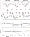 |
Fig. 8 Mean spectra and atmospheric structure for selected clusters representing wide line profiles. Each column depicts four selected clusters for each of the three simulations, in addition to the mean for the full simulation box (dashed black line). The top row shows the mean spectra for each of the clusters, while the bottom three rows show the temperature, vertical velocity, and vertical magnetic field as a function of log τ5000. The cluster numbers for each simulation are indicated in the legend of the temperature plot. |
Line FWHMs and depths for selected clusters from simulation ch012023.
Line FWHMs and depths for selected clusters from simulation nw012023.
Line FWHMs and depths for selected clusters from simulation nw072100.
3.4.2 Narrow profiles
In Fig. 9, we treat four clusters with some of the narrowest profiles from each simulation. Specifically, we show clusters #32, #57, #69, #75 from ch012023 (Fig. 4); clusters #42, #43, #90, #99 from nw012023 (Fig. 5); and clusters #8, #29, #55, #88 from nw072100 (Fig. 6).
The ch012023 case shows similarities across all four of our selected clusters. Most intriguing is the temperature, which increases from log τ5000 ≈ − 1 to a local maximum around log τ5000 ≈ − 3 before sinking to a minimum around log τ5000 ≈ − 5. There is some variation in the exact height of the maximum, between and within the clusters, but the general tendency is shared among the vast majority of the individual profiles, and stands in contrast to what we see in the other cluster families. Though it is not seen in the average quantities, a fraction of the profiles in these clusters do not follow the average decrease after reaching the maximum, but continue as hot streaks of fairly constant temperature all the way up to log τ5000 ≈ − 5, as seen for cluster #75 in Fig. 7. The vertical velocities are generally low (absolute values of <2.5 km s−1), with no obvious structure. Likewise, the vertical magnetic field is very weak (absolute values of <2.5 mT).
The nw012023 case reveals two distinct behaviors. Clusters #42 and #43 show the same sort of structure in temperature as the narrow clusters we considered for the ch012023 simulation, specifically a colder layer at the bottom going to a hotter layer above before decreasing again toward the core forming heights. However, the vertical velocities tend to be slightly stronger (absolute values of ~2.5 km s−1) and are predominantly down-flowing, with occasional upflows; furthermore, there are more instances of the hot streaks, which do not significantly decrease in temperature from the maximum in these clusters compared to those in the previous simulation. The vertical magnetic field components for these clusters do not seem to be particularly coherent, but they are moderately strong (absolute values of ~5 mT) in the heights below.
Somewhat different is the structure for clusters #90 and #99, which show consistently high temperatures throughout the line forming region, with only minor changes as a function of height. These clusters are correlated with strong downflows (υz < −5 km s−1), and quite strong vertical magnetic field strengths (absolute values of >10 mT).
A similar story is repeated for the nw072100 simulation. These are the narrowest profiles we looked at, and the temperature structure is quite similar to the two distinct types seen for the nw012023 simulation. For the flatter high temperature cases here (clusters #55 and #88 from Fig. 6), the vertical velocities do not get very large (absolute values of <2.5 km s−1) before reaching a height in excess of log τ5000 ≈ −5. However, they do contrast with the nearly zero vertical velocities for the two clusters (#8 and #29) with the lower starting temperatures. As in the nw012023 case there is a rise to a maximum in the temperature before it falls off again. This rise to a localized temperature maximum is not as strong in cluster #8 as in #29; however, it is more clearly seen when looking at the individual profiles in a manner similar to Fig. 7 than what is apparent from the averages shown in Fig. 9. Also in this case we find that the narrow profiles with high and consistent temperatures correlate with stronger vertical magnetic field strengths (absolute values >10 mT), while the cooler atmospheres are associated with weaker vertical field strengths (absolute values of <2.5 mT).
In summary, it appears that the key difference between the narrow and wide profile clusters we examined lies in the temperature structures. The wide profiles have clear negative temperature gradients with increasing height, while the narrow profiles actually tend to have either quite flat temperatures or to show an increase to a local maximum followed by a decrease.
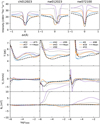 |
Fig. 9 Mean spectra and atmospheric structure for selected clusters representing narrow line profiles. The legend is the same as in Fig. 8. |
3.4.3 Shallow profiles
In Fig. 10 we look at four of the shallower clusters from each simulation. These are clusters #4, #8, #11, #30 from ch012023 (Fig. 4); clusters #4, #8, #22, #24 from nw012023 (Fig. 5); and clusters #16, #34, #36, #47 from nw072100 (Fig. 6).
In terms of the mean profiles, these clusters are some of the most similar to the observed clusters, such as #63 and #81 in Fig. 3. However, it should be noted that there is quite a lot of variance within these clusters, which becomes evident when looking at the Stokes I profiles for all the cluster members simultaneously. Even so, the amplitudes of the variations are not very large, and they retain the defining characteristic of being shallow, with small differences in intensity from the line wings to the line core. In all three simulations the temperatures tend to be lower than average across most of the formation region. On average the temperatures tend to decrease with increasing height, but there are a number of profiles that correspond to both extended and localized temperature enhancements in the range −5 < log τ5000 < −3. These temperature enhancements tend to correlate with some weak intensity enhancements around the transition from line wings to line core. In all three simulations the vertical velocities tend to be weak or moderate throughout the line forming region (absolute values of <2.5 km s−1), with the notable exception that cluster #36 from the nw072100 simulation has strong downflows (υz < −5 km s−1) in the range −5.5 < log τ5000 < −4.5 corresponding to the evident redshift of the core. Similarly, the vertical magnetic field components tend to be rather weak in all cases (absolute values of <5 mT), though there are some stronger fields (absolute values of ~5 mT) of both polarities present in the two colder clusters (#34 and #47 from nw072100).
3.4.4 Profiles with smooth transition to line core
Finally, in Fig. 11 we investigate four of the clusters showing the gentlest (most gradual) transition from line wing to line core from each simulation. These are clusters #2, #7, #9, #23 from ch012023 (Fig. 4); clusters #3, #5, #7, #22 from nw012023 (Fig. 5); and clusters #13, #14, #20, #45 from nw072100 (Fig. 6). These are fairly common types of profile, comprising about 9% of all profiles in ch012023 and nw012023, and about 7% in nw072100.
In all cases the mean temperature gradient of the cluster atmospheres is steeper than that of the full simulation box. As before, there are occasional instances of localized temperature enhancements (particularly for the nw012023 clusters), but they are infrequent. The clusters from the ch012023 and nw072100 simulations all have very weak vertical velocities (absolute values of ≪2.5 km s−1) all the way up to log τ5000 ≈ − 5, with the exception of #45 from nw072100 where stronger downflows (υz < −2.5 km s−1) appear coincidentally with the temperature enhancements around −5 < log τ5000 < −4.5. The vertical velocities in the nw012023 clusters are not very strong, but they are consistently downflowing and somewhat faster (υz > −5 km s−1) than for the other two simulations in the heights below −5 < log τ5000. For all three simulations the vertical magnetic field components appear generally quite weak (absolute values of <5 mT), though the nw012023 clusters have some moderately strong fields (absolute values of ≥5 mT) of both polarities interspersed among the members of the considered clusters.
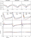 |
Fig. 10 Mean spectra and atmospheric structure for selected clusters representing shallow line profiles. The legend is the same as in Fig. 8. |
4 Discussion
Although the mean profiles on the whole correspond quite well between observations and simulations, we find that there are important differences between the observed and synthetic line profiles. Chief among them is the tendency for the synthetic profiles to be narrower than the observed profiles, both individually and in mean. This finding echoes several previous studies (e.g., Leenaarts et al. 2009; de la Cruz Rodríguez et al. 2012, 2013, 2016; Štěpán & Trujillo Bueno 2016; Jurčák et al. 2018) that investigated the correspondence between synthetic and observed Ca II 854.2 nm spectra. Another key difference is the tendency for synthetic spectra to display a sharper transition from the wing to the core (a sharp elbow); this is also seen in the results of those previous studies, but is not much commented on.
In those previous studies, the discrepancy between observed and synthetic line widths is often ascribed to the effects of numerical resolution in the simulation causing less small-scale dynamics and heating. Other possible contributions have been suggested; for example, Carlsson et al. (2015) demonstrate how the temperature profile of the atmosphere can affect Mg II profile shapes, and Carlin et al. (2013) show how lines can be broadened from temporal averaging. The effects of resolution are certainly an important element of the explanation, as we found that our 100 km resolution simulation has both a narrower mean profile and several clusters of far narrower profiles than the two 23 km resolution simulations, even though the 100 km resolution was the most vigorous and dynamic of our simulations. However, we still see the same difference in the shape of the elbow in both mean spectra of our 23 km resolution simulations and in several of their clusters, which indicates that resolution is not the only issue.
In many cases, an ad hoc microturbulence is added in the spectral synthesis to account for such missing small-scale dynamics and improve the fit between observed and synthetic profiles. For instance, de la Cruz Rodríguez et al. (2012) found that they needed a microturbulence of 3 km s−1 in order to broaden their synthetic profiles to be comparable in width to the observations of Cauzzi et al. (2009). However, as can be seen in Fig. 2 of de la Cruz Rodríguez et al. (2012), the broadening due to microturbulence does not fix the sharp elbow. Although not shown here, we repeated some of our clustering experiments after adding microturbulence in different amounts. We find the same behavior persisting throughout the clusters, namely that the elbow remains sharper for the synthetic profiles than the observed profiles, and adding micro-turbulence makes the profile wider only near the line core, resulting in profile shapes that still have an elbow that is sharper than observed.
Our investigation into the atmospheric structure for the different clusters revealed that the key parameter in setting spectral shapes that resemble the observations is the temperature stratification, in particular the temperature gradient in the region −3 ≲ log τ5000 ≲ −1. A stronger temperature gradient in this region typically leads to broader profiles and a gentle wing-to-core transition. This can be seen in our groups of clusters showing the shallow profiles (Fig. 10), or the smoothest transition from wing to core (Fig. 11), all of which have a stronger gradient than the average of each simulation. Interestingly, in their Fig. 3 Manso Sainz & Trujillo Bueno (2010) show a comparison of the Ca II 854.2 nm intensity profiles from the semi-empirical FALC and M-CO (also known as FALX) atmospheres where the M-CO result displays an appreciably smoother elbow. Compared to FALC, the M-CO atmosphere has a temperature gradient that persists into a cooler temperature minimum at 1 Mm (corresponding to log τ5000 ≈ −5.2), compared to the 500 km (corresponding to log τ5000 ≈ −3.5) of FALC (the M-CO synthetic line core has other shortcomings, such as a saturated core, that do not resemble observations). Another revealing aspect from our present work is that the broadest synthetic profiles, associated with clusters that have strong velocities (Fig. 8), are broad but still have a sharp elbow. This strongly suggests that turbulent broadening, whether by real atmospheric motions or by adding microturbulence, does not lead to the spectral shapes of observed quiet-Sun profiles.
Our analysis presents a new way to quantify differences in spatially resolved spectra that go beyond averages and use more information than simpler line properties, such as shifts or widths. This can be used as a stringent test when comparing observations and simulations, but also to learn about the formation of typical spectral shapes. A key result is that the simulations we tested show much larger variations that the observations. The shapes of the most common spectral clusters are richer for the synthetic profiles, where strongly asymmetric and emission profiles are much more common than in observations. The reason for this additional variation is not yet understood. It is also puzzling that a lower activity level in the simulations does not seem to lead to less variation in spectral shapes. However, our comparison with the most active simulation available (nw072100) is not completely fair because it has a coarser spatial resolution and an area 36 times larger than the less active simulations. Another aspect that could affect the comparison and appearance of synthetic profiles is that our synthetic spectra are an instant snapshot, while the observations were a scan through wavelength that took a few seconds to complete. We were unable to test this scanning effect with synthetic spectra at this point, but Schlichenmaier et al. (2023) find that this can affect the profiles, in particular in areas with magnetic features.
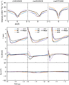 |
Fig. 11 Mean spectra and atmospheric structure for selected clusters representing the line profiles with the smoothest transition from wing to core. The legend is the same as in Fig. 8. |
5 Conclusions
We performed a comparative clustering analysis of the synthetic Ca II 854.2 nm profiles from three simulations of varying magnetic activity alongside quiet-Sun observations of the same spectral line. We found that the clusters retrieved from the observations and the simulations show similarities, but also significant differences that persist even after the synthetic profiles have been spatially and spectrally degraded to match the observational conditions.
The most obvious difference was the that the observed profiles were generally wider than the synthetic. However, we also see a tendency for the synthetic absorption profiles to display steeper transitions from the line wings to the core, while the observed absorption profiles in general had gentler transitions. Another key difference was that the observations contain far fewer profiles with emission peaks, strongly asymmetric profiles, or complex line profiles than we see in the synthetic spectra. This is a possible indication that even our quietest simulation is more dynamic than the observed region.
When we compared the synthetic profiles from the simulations with each other, we find that the largest difference between the retrieved clusters was that the more active simulations produced larger intensity differences and more variance within the clusters, but mostly the same profile shapes appeared in all of the simulations. A specific profile type with broad emission peaks is found only in the most vigorous simulation. Additionally, that simulation also had a significantly lower horizontal resolution than the other two, and produced the narrowest absorption profiles.
Furthermore, we investigated the atmospheric structure for a few selected clusters of absorption profiles: the widest, the narrowest, the shallowest, and profiles with the least steep transitions from line wing to core. We find that the strongest correlations and differences between these types of clusters appear in the temperature stratifications. Both the shallow and least steep wing to core clusters came from atmospheres with lower than average temperatures and their temperatures typically followed a monotonous negative gradient with increasing heights, with occasional occurrences of localized heating. For these clusters, the vertical velocities and vertical magnetic field components were generally quite weak throughout the line forming region. The profile shapes in these clusters are the closest to observations, which suggests that the quiet-Sun has steeper temperature gradients in the range −3 ≲ log τ5000 ≲ −1 than the simulation averages.
Among the clusters of wider profiles, we find that some clusters show weak velocities and magnetic field strengths and other clusters show stronger flows and field strengths. The profiles with the weaker velocities tend to have more prominent temperature minima, with the temperature decreasing steadily throughout the range −5 ≲ log τ5000 ≲ −2. The profiles associated with stronger velocities and field strengths coincide with higher and flatter temperatures, often reaching all the way up to around log τ5000 ≈ −5. This demonstrates that high velocities are not necessary ingredients for producing wide profiles.
For the clusters with the narrowest profiles we find that the temperature stratification took on a markedly different character compared to the other clusters we have considered. In the cases where the velocities and magnetic field strengths were weak, the temperature tends to rise to a significantly higher-than-average local maximum around log τ5000 ≈ −3 before sinking again. In the cases where the vertical velocities and magnetic field strengths took on higher values, the temperatures took on and maintain quite constant and high values throughout the whole line forming region. This shows that strong velocities alone are not sufficient to produce wide profiles.
In sum, we find indications that the temperature stratification, more so than the vertical velocities, holds the key for getting the simulations to produce synthetic Ca II 854.2 nm profiles more similar to the quiet-Sun observations.
Acknowledgements
We wish to thank the anonymous referee for constructive and thorough feedback, which lead to several improvements of this manuscript. This work has been supported by the Research Council of Norway through its Centers of Excellence scheme, project number 262622. Computational resources have been provided by UNINETT Sigma2 - the National Infrastructure for High Performance Computing and Data Storage in Norway. The computations were enabled by resources provided by the Swedish National Infrastructure for Computing (SNIC) at the PDC Centre for High Performance Computing (PDC-HPC) at the Royal Institute of Technology partially funded by the Swedish Research Council through grant agreement no. 2018-05973. The Swedish 1-m Solar Telescope is operated on the island of La Palma by the Institute for Solar Physics of Stockholm University in the Spanish Observatorio del Roque de los Muchachos of the Instituto de Astrofísica de Canarias. The Institute for Solar Physics is supported by a grant for research infrastructures of national importance from the Swedish Research Council (registration number 2021-00169).
Appendix A The clusters for the degraded synthetic profiles
In Sect. 3.3, we present the resulting clusters after applying k-means to our observed profiles and to our undegraded synthetic profiles. We performed the same type of clustering also for synthetic profiles that were spectrally and spatially degraded and downsampled to match the observational conditions, and the results are shown in Figs. A.1, A.2, and A.3. The net effect of the degradation is primarily manifested as a reduction in the variance of the profiles with regards to absolute intensity. However, the general shapes persist from the undegraded clusters, and the qualitative differences between the observed and synthetic line profiles remain similar. Notably, there are still far more exotic profiles present in the degraded clusters compared to the distribution that is seen in the observations.
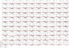 |
Fig. A.1 k-means clusters of synthetic Ca II 854.2 nm intensity profiles, using 100 clusters for the unnormalized and degraded profiles from ch012023. The red line is the cluster mean, and the black lines are all the individual profiles belonging to each cluster. The gray line indicates the position of λ0. |
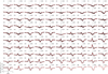 |
Fig. A.2 k-means clusters of synthetic Ca II 854.2 nm intensity profiles, using 100 clusters for the unnormalized and degraded profiles from nw012023. The red line is the cluster mean, and the black lines are all the individual profiles belonging to each cluster. The gray line indicates the position of λ0. |
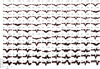 |
Fig. A.3 k-means clusters of synthetic Ca II 854.2 nm intensity profiles, using 100 clusters for the unnormalized and degraded profiles from nw072100. The red line is the cluster mean, and the black lines are all the individual profiles belonging to each cluster. The gray line indicates the position of λ0. |
Appendix B Additional figures of atmospheric structure
In Fig. B.1 we show the spectra and atmospheric profiles from four clusters from the nw072100 simulation, which include a shallow absorption profile and more dynamic clusters with broad emission.
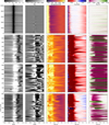 |
Fig. B.1 Atmospheric structure of clusters #15, #93, #94, #96 in Fig. 6. The top panel contains a cluster of the typical absorption profiles, while the three bottom panels are the clusters showing broad emission in nw072100, following the same presentation as in Fig. 7. |
Appendix C A few results from using k-Shape
This section shows a few examples of the clusters retrieved by using k-Shape on z-normalized spectra. Compared to the k-means results (where spectra were not normalized), there are more complicated shapes present in these clusters, which for the most part are hidden in the least constrained and most shallow clusters in the original cases shown in the main text.
As examples, Fig. C.1 shows cluster #28, which primarily corresponds to #81 and #97 in Fig. 3; #25 mostly corresponds to #89, #97, #99; #94 mostly goes into #90, #97, #100; and #16 for the most part splits into #17, #45, #60, #63, #81. Figure C.2 has unique clusters, such as #19, #46, #64, #75, #77, #85, and #100, which do not appear with corresponding centroids in Fig. 4. Cluster #19 is quite well spread out, but the larger receivers are #21, #44, #50, #55, #73, #92; #46 goes mostly into #13; #64 goes into many different clusters, but the larger receivers are #3, #7, #28, #30, #33, and #34; #75 goes primarily into #81, #99; #77 goes mostly into #30, #35, #55, #73; #85 is also quite spread out with the most frequent destinations being #14, #25, #27, #55; and #100 goes mostly into #13, #29, #62. Even after degradation, the same complex shapes still appear as seen in Fig. C.3. We did not perform more than a cursory inspection for the other synthesized spectra, but at a preliminary glance similar trends seem to hold for these as well.
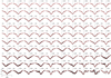 |
Fig. C.1 Clusters found with k = 100 clusters using k-Shape with ten re-initializations on the z-normalized observed spectra. |
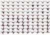 |
Fig. C.2 Clusters found with k = 100 clusters using k-Shape with a single initialization on the z-normalized undegraded spectra for the ch012023 simulation. |
 |
Fig. C.3 Clusters found with k = 100 clusters using k-Shape with a single initialization on the z-normalized degraded spectra for the ch012023 simulation. |
References
- Arthur, D., & Vassilvitskii, S. 2007, in Proceedings of the Eighteenth Annual ACM-SIAM Symposium on Discrete Algorithms, SODA ’07 (USA: Society for Industrial and Applied Mathematics), 1027 [Google Scholar]
- Asplund, M., Nordlund, Å., Trampedach, R., Allende Prieto, C., & Stein, R. F. 2000, A & A, 359, 729 [NASA ADS] [Google Scholar]
- Bjørgen, J. P., Sukhorukov, A. V., Leenaarts, J., et al. 2018, A & A, 611, A62 [CrossRef] [EDP Sciences] [Google Scholar]
- Carlin, E. S., Asensio Ramos, A., & Trujillo Bueno, J. 2013, ApJ, 764, 40 [NASA ADS] [CrossRef] [Google Scholar]
- Carlsson, M., Leenaarts, J., & De Pontieu, B. 2015, ApJ, 809, L30 [NASA ADS] [CrossRef] [Google Scholar]
- Cauzzi, G., Reardon, K. P., Uitenbroek, H., et al. 2008, A & A, 480, 515 [NASA ADS] [CrossRef] [EDP Sciences] [Google Scholar]
- Cauzzi, G., Reardon, K., Rutten, R. J., Tritschler, A., & Uitenbroek, H. 2009, A & A, 503, 577 [NASA ADS] [CrossRef] [EDP Sciences] [Google Scholar]
- Chae, J., Park, H.-M., Ahn, K., et al. 2013, Sol. Phys., 288, 89 [NASA ADS] [CrossRef] [Google Scholar]
- Cheung, M. C. M., Martínez-Sykora, J., Testa, P., et al. 2022, ApJ, 926, 53 [NASA ADS] [CrossRef] [Google Scholar]
- de la Cruz Rodríguez, J., Socas-Navarro, H., Carlsson, M., & Leenaarts, J. 2012, A & A, 543, A34 [CrossRef] [EDP Sciences] [Google Scholar]
- de la Cruz Rodríguez, J., De Pontieu, B., Carlsson, M., & Rouppe van der Voort, L. H. M. 2013, ApJ, 764, L11 [CrossRef] [Google Scholar]
- de la Cruz Rodríguez, J., Hansteen, V., Bellot-Rubio, L., & Ortiz, A. 2015a, ApJ, 810, 145 [CrossRef] [Google Scholar]
- de la Cruz Rodríguez, J., Löfdahl, M. G., Sütterlin, P., Hillberg, T., & Rouppe van der Voort, L. 2015b, A & A, 573, A40 [CrossRef] [EDP Sciences] [Google Scholar]
- de la Cruz Rodríguez, J., Leenaarts, J., & Asensio Ramos, A. 2016, ApJ, 830, L30 [Google Scholar]
- De Pontieu, B., Title, A. M., Lemen, J. R., et al. 2014, Sol. Phys., 289, 2733 [Google Scholar]
- De Pontieu, B., Testa, P., Martínez-Sykora, J., et al. 2022, ApJ, 926, 52 [NASA ADS] [CrossRef] [Google Scholar]
- Fontenla, J. M., Avrett, E. H., & Loeser, R. 1993, ApJ, 406, 319 [Google Scholar]
- Gudiksen, B. V., Carlsson, M., Hansteen, V. H., et al. 2011, A & A, 531, A154 [NASA ADS] [CrossRef] [EDP Sciences] [Google Scholar]
- Hansteen, V. H., Martinez-Sykora, J., Carlsson, M., et al. 2023, ApJ, 944, 131 [NASA ADS] [CrossRef] [Google Scholar]
- Iijima, H., & Yokoyama, T. 2015, ApJ, 812, L30 [NASA ADS] [CrossRef] [Google Scholar]
- Jurčák, J., Štěpán, J., Trujillo Bueno, J., & Bianda, M. 2018, A & A, 619, A60 [CrossRef] [EDP Sciences] [Google Scholar]
- Khomenko, E., Vitas, N., Collados, M., & de Vicente, A. 2018, A & A, 618, A87 [NASA ADS] [CrossRef] [EDP Sciences] [Google Scholar]
- Kuridze, D., Henriques, V., Mathioudakis, M., et al. 2017, ApJ, 846, 9 [Google Scholar]
- Leenaarts, J., & Carlsson, M. 2009, ASP Conf. Ser., 415, 87 [Google Scholar]
- Leenaarts, J., Carlsson, M., Hansteen, V., & Rouppe van der Voort, L. 2009, ApJ, 694, L128 [NASA ADS] [CrossRef] [Google Scholar]
- Leenaarts, J., Carlsson, M., & Rouppe van der Voort, L. 2012, ApJ, 749, 136 [NASA ADS] [CrossRef] [Google Scholar]
- Leenaarts, J., Pereira, T. M. D., Carlsson, M., Uitenbroek, H., & De Pontieu, B. 2013a, ApJ, 772, 89 [NASA ADS] [CrossRef] [Google Scholar]
- Leenaarts, J., Pereira, T. M. D., Carlsson, M., Uitenbroek, H., & De Pontieu, B. 2013b, ApJ, 772, 90 [NASA ADS] [CrossRef] [Google Scholar]
- Leenaarts, J., de la Cruz Rodríguez, J., Kochukhov, O., & Carlsson, M. 2014, ApJ, 784, L17 [NASA ADS] [CrossRef] [Google Scholar]
- Lin, H.-H., & Carlsson, M. 2015, ApJ, 813, 34 [NASA ADS] [CrossRef] [Google Scholar]
- Lin, H.-H., Carlsson, M., & Leenaarts, J. 2017, ApJ, 846, 40 [NASA ADS] [CrossRef] [Google Scholar]
- MacQueen, J. 1967, Proceedings of the Fifth Berkeley Symposium on Mathematical Statistics and Probability, eds. L. M. Le Cam, & J. Neyman, (University of California Press), 1, 281 [Google Scholar]
- Manso Sainz, R., & Trujillo Bueno, J. 2010, ApJ, 722, 1416 [NASA ADS] [CrossRef] [Google Scholar]
- Moe, T. E., Pereira, T. M. D., & Carlsson, M. 2022, A & A, 662, A80 [NASA ADS] [CrossRef] [EDP Sciences] [Google Scholar]
- Moe, T. E., Pereira, T. M. D., Calvo, F., & Leenaarts, J. 2023, A & A, 675, A130 [NASA ADS] [CrossRef] [EDP Sciences] [Google Scholar]
- Molnar, M. E., Reardon, K. P., Cranmer, S. R., et al. 2021, ApJ, 920, 125 [NASA ADS] [CrossRef] [Google Scholar]
- Paparrizos, J., & Gravano, L. 2015, in Proceedings of the 2015 ACM SIGMOD International Conference on Management of Data, SIGMOD ’15 (New York, NY, USA: Association for Computing Machinery), 1855 [CrossRef] [Google Scholar]
- Pedregosa, F., Varoquaux, G., Gramfort, A., et al. 2011, J. Mach. Learn. Res., 12, 2825 [Google Scholar]
- Pereira, T. M. D., Asplund, M., Collet, R., et al. 2013a, A & A, 554, A118 [NASA ADS] [CrossRef] [EDP Sciences] [Google Scholar]
- Pereira, T. M. D., Leenaarts, J., De Pontieu, B., Carlsson, M., & Uitenbroek, H. 2013b, ApJ, 778, 143 [NASA ADS] [CrossRef] [Google Scholar]
- Pereira, T. M. D., Carlsson, M., De Pontieu, B., & Hansteen, V. 2015, ApJ, 806, 14 [NASA ADS] [CrossRef] [Google Scholar]
- Przybylski, D., Cameron, R., Solanki, S. K., et al. 2022, A & A, 664, A91 [NASA ADS] [CrossRef] [EDP Sciences] [Google Scholar]
- Quintero Noda, C., Shimizu, T., de la Cruz Rodríguez, J., et al. 2016, MNRAS, 459, 3363 [NASA ADS] [CrossRef] [Google Scholar]
- Rathore, B., & Carlsson, M. 2015, ApJ, 811, 80 [NASA ADS] [CrossRef] [Google Scholar]
- Rathore, B., Carlsson, M., Leenaarts, J., & De Pontieu, B. 2015a, ApJ, 811, 81 [NASA ADS] [CrossRef] [Google Scholar]
- Rathore, B., Pereira, T. M. D., Carlsson, M., & De Pontieu, B. 2015b, ApJ, 814, 70 [NASA ADS] [CrossRef] [Google Scholar]
- Scharmer, G. B., Bjelksjö, K., Korhonen, T. K., Lindberg, B., & Petterson, B. 2003, Proc. SPIE, 4853, 341 [NASA ADS] [CrossRef] [Google Scholar]
- Scharmer, G. B., Narayan, G., Hillberg, T., et al. 2008, ApJ, 689, L69 [Google Scholar]
- Schlichenmaier, R., Pitters, D., Borrero, J. M., & Schubert, M. 2023, A & A, 669, A78 [NASA ADS] [CrossRef] [EDP Sciences] [Google Scholar]
- Štěpán, J. & Trujillo Bueno, J. 2016, ApJ, 826, L10 [CrossRef] [Google Scholar]
- Stein, R. F., & Nordlund, Å. 1998, ApJ, 499, 914 [Google Scholar]
- Steinhaus, H. 1956, Bulletin de l’Académie Polonaise des Sciences, 3, 801 [Google Scholar]
- Tavenard, R., Faouzi, J., Vandewiele, G., et al. 2020, J. Mach. Learn. Res., 21, 1 [Google Scholar]
- Uitenbroek, H. 1989, A & A, 213, 360 [NASA ADS] [Google Scholar]
- van Noort, M., Rouppe van der Voort, L., & Löfdahl, M. G. 2005, Sol. Phys., 228, 191 [Google Scholar]
- Vögler, A., Bruls, J. H. M. J., & Schüssler, M. 2004, A & A, 421, 741 [CrossRef] [EDP Sciences] [Google Scholar]
- Wedemeyer-Böhm, S. & Carlsson, M. 2011, A & A, 528, A1 [CrossRef] [EDP Sciences] [Google Scholar]
All Tables
All Figures
|
Fig. 1 Overview of the observed region. The images show the field of view used for the spectral clustering, at 2023-06-24T09:15. Top: Ca II 854.2 nm line core intensity. Bottom: Fe I 630.2 nm line wing Stokes V, a proxy for magnetic field. |
| In the text | |
|
Fig. 2 Mean spectra with 1σ variations for observations and three simulations. The shaded bands show, for each wavelength, the 1σ range of departures from the mean. All spectra were normalized to the local continuum at λ0 + 0.1 nm. The synthetic spectra were degraded to match the conditions of the observations. |
| In the text | |
|
Fig. 3 k-means clusters of Ca II 854.2 nm observed spectra, using 100 clusters, sorted from most to least frequent. The red line denotes the average of all line profiles belonging to each cluster (thin black lines). The fraction of all profiles belonging to each cluster is indicated as a percentage next to the cluster number. The gray line indicates the position of λ0, the rest wavelength. |
| In the text | |
|
Fig. 4 k-means clusters of Ca II 854.2 nm synthetic spectra from the ch012023 simulation. The legend is the same as in Fig.3. |
| In the text | |
|
Fig. 5 k-means clusters of Ca II 854.2 nm synthetic spectra from the nw012023 simulation. The legend is the same as in Fig. 3. |
| In the text | |
|
Fig. 6 k-means clusters of Ca II 854.2 nm synthetic spectra from the nw072100 simulation. The legend is the same as in Fig. 3. |
| In the text | |
|
Fig. 7 Individual spectra and atmospheric structure of selected clusters from the ch0l2023 simulation. From left to right, the first two columns show the Stokes I and V (normalized to the nearby continuum, around λ0 + 0.95 nm), while the last three columns show the temperature, vertical velocity, and vertical magnetic field as a function of log τ5000. Each row depicts a different cluster. From the top, the first and second are #80 and #84 (from the numbering in Fig. 4), and represent some of the wider line profiles. The third and fourth rows depict cluster numbers #57 and #75, which represent some of the narrowest line profiles. |
| In the text | |
|
Fig. 8 Mean spectra and atmospheric structure for selected clusters representing wide line profiles. Each column depicts four selected clusters for each of the three simulations, in addition to the mean for the full simulation box (dashed black line). The top row shows the mean spectra for each of the clusters, while the bottom three rows show the temperature, vertical velocity, and vertical magnetic field as a function of log τ5000. The cluster numbers for each simulation are indicated in the legend of the temperature plot. |
| In the text | |
|
Fig. 9 Mean spectra and atmospheric structure for selected clusters representing narrow line profiles. The legend is the same as in Fig. 8. |
| In the text | |
|
Fig. 10 Mean spectra and atmospheric structure for selected clusters representing shallow line profiles. The legend is the same as in Fig. 8. |
| In the text | |
|
Fig. 11 Mean spectra and atmospheric structure for selected clusters representing the line profiles with the smoothest transition from wing to core. The legend is the same as in Fig. 8. |
| In the text | |
|
Fig. A.1 k-means clusters of synthetic Ca II 854.2 nm intensity profiles, using 100 clusters for the unnormalized and degraded profiles from ch012023. The red line is the cluster mean, and the black lines are all the individual profiles belonging to each cluster. The gray line indicates the position of λ0. |
| In the text | |
|
Fig. A.2 k-means clusters of synthetic Ca II 854.2 nm intensity profiles, using 100 clusters for the unnormalized and degraded profiles from nw012023. The red line is the cluster mean, and the black lines are all the individual profiles belonging to each cluster. The gray line indicates the position of λ0. |
| In the text | |
|
Fig. A.3 k-means clusters of synthetic Ca II 854.2 nm intensity profiles, using 100 clusters for the unnormalized and degraded profiles from nw072100. The red line is the cluster mean, and the black lines are all the individual profiles belonging to each cluster. The gray line indicates the position of λ0. |
| In the text | |
|
Fig. B.1 Atmospheric structure of clusters #15, #93, #94, #96 in Fig. 6. The top panel contains a cluster of the typical absorption profiles, while the three bottom panels are the clusters showing broad emission in nw072100, following the same presentation as in Fig. 7. |
| In the text | |
|
Fig. C.1 Clusters found with k = 100 clusters using k-Shape with ten re-initializations on the z-normalized observed spectra. |
| In the text | |
|
Fig. C.2 Clusters found with k = 100 clusters using k-Shape with a single initialization on the z-normalized undegraded spectra for the ch012023 simulation. |
| In the text | |
|
Fig. C.3 Clusters found with k = 100 clusters using k-Shape with a single initialization on the z-normalized degraded spectra for the ch012023 simulation. |
| In the text | |
Current usage metrics show cumulative count of Article Views (full-text article views including HTML views, PDF and ePub downloads, according to the available data) and Abstracts Views on Vision4Press platform.
Data correspond to usage on the plateform after 2015. The current usage metrics is available 48-96 hours after online publication and is updated daily on week days.
Initial download of the metrics may take a while.