| Issue |
A&A
Volume 682, February 2024
|
|
|---|---|---|
| Article Number | A21 | |
| Number of page(s) | 15 | |
| Section | Cosmology (including clusters of galaxies) | |
| DOI | https://doi.org/10.1051/0004-6361/202346931 | |
| Published online | 31 January 2024 | |
Field-level Lyman-α forest modeling in redshift space via augmented nonlocal Fluctuating Gunn-Peterson Approximation
1
Instituto de Astrofísica de Canarias, Calle Via Láctea s/n, 38205 La Laguna, Tenerife, Spain
e-mail: This email address is being protected from spambots. You need JavaScript enabled to view it.
2
Departamento de Astrofísica, Universidad de La Laguna, 38206 La Laguna, Tenerife, Spain
3
Department of Physics and Astronomy, Universitá degli Studi di Padova, Vicolo dell’Osservatorio 3, 35122 Padova, Italy
e-mail: This email address is being protected from spambots. You need JavaScript enabled to view it.
4
INAF – Osservatorio Astronomico di Padova, Vicolo dell’Osservatorio 5, 35122 Padova, Italy
5
Theoretical Astrophysics, Department of Earth and Space Science, Graduate School of Science, Osaka University, 1-1 Machikaneyama, Toyonaka, Osaka 560-0043, Japan
6
Kavli-IPMU (WPI), University of Tokyo, 5-1-5 Kashiwanoha, Kashiwa, Chiba 277-8583, Japan
7
Department of Physics & Astronomy, University of Nevada, Las Vegas, 4505 S. Maryland Pkwy, Las Vegas, NV 89154-4002, USA
Received:
17
May
2023
Accepted:
10
October
2023
Abstract
Context. Devising fast and accurate methods of predicting the Lyman-α forest at the field level, avoiding the computational burden of running large-volume cosmological hydrodynamic simulations, is of fundamental importance to quickly generate the massive set of simulations needed by the state-of-the-art galaxy and Lyα forest spectroscopic surveys.
Aims. We present an improved analytical model to predict the Lyα forest at the field level in redshift space from the dark matter field, expanding upon the widely used Fluctuating Gunn-Peterson Approximation (FGPA). Instead of assuming a unique universal relation over the whole considered cosmic volume, we introduce a dependence on the cosmic web environment (knots, filaments, sheets, and voids) in the model, thereby effectively accounting for nonlocal bias. Furthermore, we include a detailed treatment of velocity bias in the redshift space distortion modeling, allowing the velocity bias to be cosmic-web-dependent.
Methods. We first mapped the dark matter field from real to redshift space through a particle-based relation including velocity bias, depending on the cosmic web classification of the dark matter field in real space. We then formalized an appropriate functional form for our model, building upon the traditional FGPA and including a cutoff and a boosting factor mimicking a threshold and inverse-threshold bias effect, respectively, with model parameters depending on the cosmic web classification in redshift space. Eventually, we fit the coefficients of the model via an efficient Markov chain Monte Carlo scheme.
Results. We find evidence for a significant difference between the same model parameters in different environments, suggesting that for the investigated setup the simple standard FGPA is not able to adequately predict the Lyα forest in the different cosmic web regimes. We reproduce the summary statistics of the reference cosmological hydrodynamic simulation that we use for comparison, yielding an accurate mean transmitted flux, probability distribution function, 3D power spectrum, and bispectrum. In particular, we achieve maximum deviation and average deviation accuracy in the Lyα forest 3D power spectrum of ∼3% and ∼0.1% up to k ∼ 0.4 h Mpc−1, and ∼5% and ∼1.8% up to k ∼ 1.4 h Mpc−1.
Conclusions. Our new model outperforms previous analytical efforts to predict the Lyα forest at the field level in all the probed summary statistics, and has the potential to become instrumental in the generation of fast accurate mocks for covariance matrices estimation in the context of current and forthcoming Lyα forest surveys.
Key words: large scale structure of Universe / dark energy / quasars: emission lines / surveys / methods: numerical
© The Authors 2024
 Open Access article, published by EDP Sciences, under the terms of the Creative Commons Attribution License (https://creativecommons.org/licenses/by/4.0), which permits unrestricted use, distribution, and reproduction in any medium, provided the original work is properly cited.
This article is published in open access under the Subscribe to Open model. This email address is being protected from spambots. You need JavaScript enabled to view it. to support open access publication.
1. Introduction
The neutral hydrogen (H I) absorption features imprinted in quasar spectra, also known as the Lyman-α forest (Lyα forest), represent promising cosmological probes over the current and next decades. The Lyα forest traces the density field continuously along the line of sight, and the high number density of quasar sight lines per square degree delivered by state-of-the-art cosmological redshift surveys will allow building accurate three-dimensional maps of the Universe at z ≳ 1.8, in other words, at distances that are currently beyond the reach of wide-field galaxy redshift surveys. In the wait of next-generation astronomical facilities such as the Square Kilometre Array Observatory1 and the Extremely Large Telescope2, the Lyα forest is anticipated to play a pivotal role in refining the constraints on cosmological models and advancing our comprehension of the high-redshift Universe.
To maximize the scientific return and optimize the extraction of cosmological information from the unprecedented incoming Lyα forest datasets provided by surveys as DESI (Levi et al. 2013), Euclid (Amendola et al. 2018), WEAVE-QSO (Pieri et al. 2016), and Subaru-PFS (Takada et al. 2014), it is extremely important to develop accurate analytical models and numerical tools to efficiently interpret and analyze Lyα forest observables.
In particular, a primary goal is to formalize an effective model of the bias relation linking the Lyα forest to the dark matter field. In fact, an effective bias mapping allows the prediction of the Lyα forest from the dark matter field in a fast and accurate way, enabling the generation of massive sets of Lyα forest mock lightcones. Mock catalogs have become the standard tool used in large-scale cosmological surveys to robustly address uncertainties on cosmological parameters, to test pipelines and commissioning tools, and to assess the feasibility of studies targeting new observables, among others. Furthermore, knowing an effective bias description makes it possible to forward-model the Lyα forest at the field level and iteratively reconstruct the Lyα forest (see e.g., Horowitz et al. 2019; Porqueres et al. 2020) and its baryon acoustic oscillations (BAOs), improving on methods of de-evolving cosmic structures back in time with some approximation for the displacement field (e.g., Eisenstein et al. 2007, and later works implementing higher-order Lagrangian perturbation theory refinements).
In addition, the dark matter field – Lyα forest connection has found an interesting application in tomographic studies as well, such as in the LATIS survey (Newman et al. 2020), in the CLAMATO survey (Lee et al. 2018; Horowitz et al. 2022b), and in the PSF Galaxy Evolution Survey (Greene et al. 2022).
Pioneering studies (Hui & Gnedin 1997; Rauch 1998; Croft et al. 1998; Weinberg et al. 1999) proposed to model the Lyα forest using a deterministic scaling relation mapping – known as Fluctuating Gunn-Peterson Approximation (FGPA) – between the dark matter density and the H I optical depth. While useful, fairly accurate on large linear scales, and fast to compute, the FGPA has been shown to lose accuracy and not adequately model the summary statistics of the Lyα forest in the weakly nonlinear regime (k > 0.1 h Mpc−1) (e.g., Sinigaglia et al. 2022). A plethora of works employed the FGPA to forward-model the Lyα forest from dark matter density fields obtained through N-body simulations (Meiksin & White 2001; Viel et al. 2002; Slosar et al. 2009; White et al. 2010; Rorai et al. 2013; Lee et al. 2014), approximated gravity solvers (Horowitz et al. 2019), and Gaussian or lognormal random fields (Le Goff et al. 2011; Font-Ribera et al. 2012; Farr et al. 2020). In particular, the LYALPHA-COLORE method (Farr et al. 2020), applying the FGPA to lognormal fields, with free parameters constrained so as to match the position and width of the acoustic peak in the Lyα forest two-point correlation function and the amplitude of the 1D Lyα forest power spectrum, was adopted to produce the mock lightcones used for the BAO measurements of the Lyα forest from the final eBOSS data release (SDSS DR16; du Mas des Bourboux et al. 2020).
On the other hand, more sophisticated iterative methods of modeling the Lyα forest, employing different strategies, have been proposed, such as for example LYMAS (Peirani et al. 2014, 2022) and the Iteratively-Matched Statistics (Ims, Sorini et al. 2016). These techniques have been shown to yield promising results, although they still feature deviations of 5 − 20% in the 3D power spectrum. Moreover, these techniques were not applied to approximated gravity solvers, but rely on full N-body simulations. Therefore, they are not able to overcome the computational burden of running massive sets of simulations.
With the flourishing of machine learning methods, and the extraordinary attention that this field is receiving in astrophysics, the generation of AI3-accelerated simulated cosmological volumes is witnessing a rapid expansion.
The machine learning method BAM (Balaguera-Antolínez et al. 2018, 2019; Pellejero-Ibañez et al. 2020; Kitaura et al. 2022) and its extension to hydrodynamics HYDRO-BAM (Sinigaglia et al. 2021, 2022), which combines the latest version of a bias mapping method with a physically motivated, strongly supervised learning strategy and the exploitation of the hierarchy of baryon quantities, has been shown to model two- and three-point statistics to 1% and ∼10% levels of accuracy, respectively. Therefore, this technique represents a promising way forward of producing Lyα forest mock catalogs for the next-generation surveys (see e.g., Balaguera-Antolínez et al. 2023, for a concrete application to halo mock catalog generation for the DESI survey).
Deep learning has also achieved competitive results. Harrington et al. (2022) employed deep convolutional generative adversarial networks to learn how to correct the FGPA, feeding the density and velocity DM fields as inputs. In a companion paper, Horowitz et al. (2022a) exploited the idea of image generation behind deep generative methods and built a conditional convolutional auto-encoder, able to sample representations in latent space of the hydrodynamic fields of a simulation and synthesize the Lyα forest with a deep posterior distribution mapping.
Nonetheless, machine learning techniques to date still require an adequately large training set in order to appropriately address the issue of overfitting, making them expensive in the case of predicting the Lyα forest.
In this work we propose to elaborate on the FGPA formalism, augmenting it in light of the recent findings on the importance of accounting for long-range and short-range nonlocal terms in the mapping of dark matter tracers (see e.g., Balaguera-Antolínez et al. 2019; Kitaura et al. 2022; Sinigaglia et al. 2021). In particular, we explicitly introduce the dependence on the cosmic web environments through the cosmic web classification (Hahn et al. 2007) in the FGPA modeling. We showcase the application of our algorithm to map the Lyα forest on a mesh of a few Mpc cells in redshift space, and assess its accuracy by evaluating the deviation of relevant summary statistics (mean transmitted flux, probability distribution function, power spectrum, and bispectrum) of the predictions from the ones of a reference cosmological hydrodynamic simulation.
The paper is organized as follows. Section 2 introduces the cosmological hydrodynamic simulation we use to validate our method. Section 3 summarizes the cosmic web classification and its connection to nonlocal bias. In Sect. 4 we review the FGPA and describe our improvements in modeling redshift space distortions (RSDs) and nonlocal bias terms. Section 5 presents the analysis, the results of our predictions, and a discussion of them. In Sect. 6 we describe how to apply our machinery to the generation of Lyα forest simulations with lightcone geometry. Section 7 discusses potential future improvements for our model. We conclude in Sect. 8.
2. Reference cosmological hydrodynamic simulation
In this section, we present our reference cosmological hydrodynamic simulation.
The reference simulation was run with the cosmological smoothed-particle hydrodynamics (SPH) code GADGET3-OSAKA (Aoyama et al. 2018; Shimizu et al. 2019), a modified version of GADGET-3 and a descendant of the popular N-body/SPH code GADGET-2 (Springel 2005). It embeds a comoving volume, V = (500 h−1 Mpc)3, and N = 2 × 10243 particles of mass mDM = 8.43 × 10⁹ h−1 M⊙ for DM particles and mgas = 1.57 × 10⁹ h−1 M⊙ for gas particles. The gravitational softening length was set to ϵg = 16 h−1 kpc (comoving), but we allowed the baryonic smoothing length to become as small as 0.1ϵg. This means that the minimum baryonic smoothing at z = 2 is about physical 533 h−1 pc. The star formation and supernova feedback were treated as described in Shimizu et al. (2019). The code also contains important refinements, such as the density-independent formulation of SPH and the time-step limiter (Saitoh & Makino 2009, 2013; Hopkins et al. 2013).
The main baryonic processes that shape the evolution of the gas are photo-heating, photo-ionization under the UV background radiation Haardt & Madau (2012), and radiative cooling. All of these processes are accounted for and solved by the Grackle library4 (Smith et al. 2017), which determines the chemistry for atomic (H, D and He) and molecular (H2 and HD) species. The chemical enrichment from supernovae is also treated with the CELib chemical evolution library by Saitoh (2017). The initial conditions are generated at redshift z = 99 using MUSIC2 (Hahn et al. 2021), with cosmological parameters taken from Planck Collaboration VI (2020).
In this work we used the output at z = 2 (for which the computation times amount to ∼1.44 × 10⁵ CPU hours), reading both gas and dark matter properties.
To compute the Lyα forest flux field F = exp(−τ)5, we first obtained the H I optical depth, τ, by means of a line-of-sight integration as follows (Nagamine et al. 2021):
 (1)
(1)
where e, me, c, nHI, f, xj, and Δl denote, respectively, the electron charge, electron mass, speed of light in vacuum, H I number density, absorption oscillator strength, line-of-sight coordinate of the jth cell, and the physical cell size. The Voigt-line profile, ϕ(x), in Eq. (1) was provided by the fitting formula of Tasitsiomi (2006). Where necessary, relevant quantities (e.g., H I number density) were previously interpolated on the mesh according to the SPH kernel of the simulation. The coordinates, xj, of cells along the line of sight refer to the outcome of the interpolation of particles based either on their positions in real space, rj, or redshift space,  , where
  , a, and H are the jth particle velocity components along the line of sight, the scale factor, and the Hubble parameter at z = 2, respectively.
We interpolated the dark matter and the Lyα forest fields in real and in redshift space onto a 2563-cell cubic mesh using a CIC mass assignment scheme (Hockney & Eastwood 1981). Such a resolution corresponds to a physical cell-volume of ∂V ∼ (1.95 h−1 Mpc)3 and a Nyquist frequency of knyq ∼ 1.6 h Mpc−1.
It is worth noting that the simulations utilized for the analyses of the Lyα forest in Momose et al. (2021), Nagamine et al. (2021), the exploration of the cosmological H I distribution in Ando et al. (2019), and the examination of bias in cosmological gas tracers in Sinigaglia et al. (2021, 2022) were all executed using the same code.
3. Cosmic web classification and nonlocal bias
The cosmic web (see e.g., Bond et al. 1996) arises as a result of gravitational instability and the formation and growth of cosmic structures from tiny perturbations of the primordial matter density field in the early Universe. While several different methods have been proposed in the literature to mathematically define the cosmic web (see Cautun et al. 2014; Libeskind et al. 2017, for a summary), we focus here on the following procedure.
To quantitatively describe the large-scale matter distribution and split it into different cosmic web environments, Hahn et al. (2007) proposed a classification scheme based on the signature of the eigenvalues of the gravitational tidal field tensor,
 (2)
(2)
where ϕ denotes the gravitational potential and r stands for Eulerian coordinates. Considering the equations of motion in comoving coordinates
 (3)
(3)
for a test particle subject to the gravitational potential, ϕ, and assuming ∇ϕ(r) = 0 at the center of mass of dark matter haloes (i.e., there is a local minimum), one can linearize the equation of motions and realize that the dynamics close to local extrema of the gravitational potential in the linear regime is ruled by the three eigenvalues λi (i = 1, 2, 3) of 𝒯ij (we refer the reader to Hahn et al. 2007, for more details on the calculations). In a close analogy to the Zel’dovich approximation (Zel’dovich 1970), and sorting the λi in decreasing order such that λ1 ≥ λ2 ≥ λ3, Hahn et al. (2007) defined a region at coordinates r to belong to:
-
a knot, if λ1, λ2 λ3 ≥ 0;
-
a filament, if λ1, λ2 ≥ 0, λ3 < 0;
-
a sheet, if λ1 ≥ 0, λ2, λ3 < 0;
-
a void, if λ1, λ2, λ3 < 0.
At this point, one can drop the assumption of local extrema at the center of mass of the dark matter halo and generalize the cosmic web classification to any point in the density field. This implies the emergence of a constant additive acceleration term to the linearized equations of motion, which however does not affect the role played by the tidal tensor in linear order.
Elaborating on this work, Forero-Romero et al. (2009) proposed to relax the threshold for classifying the cosmic web, based on simple dynamical arguments and realizing that raising the threshold from λth = 0 to λth = 0.1 provides a classification that better matches the visual appearance of the cosmic web.
The T-web classification has been widely adopted to investigate the properties of dark matter haloes, galaxies, and intergalactic gas in the cosmic web (Hahn et al. 2007; Yang et al. 2017; Martizzi et al. 2019; Sinigaglia et al. 2021), to develop fast, accurate bias models to generate haloes and galaxy mock catalogs (e.g., Zhao et al. 2015; Balaguera-Antolínez et al. 2018, 2019, 2023; Pellejero-Ibañez et al. 2020; Kitaura et al. 2022), and to perform observational cosmological analysis (e.g., Lee & White 2016; Krolewski et al. 2017; Horowitz et al. 2019), among other things.
The T-web classification has also been shown to provide a direct connection between the phenomenology of the cosmic web and the mathematical description of halo bias relying on Eulerian perturbation theory (see e.g., McDonald & Roy 2009). In fact, discriminating between different T-web environments corresponds to considering a perturbative bias expansion up to the third order, including both local and nonlocal long-range bias terms. In this sense, following Kitaura et al. (2022), we denote the three invariants of the tidal field tensor as:
-
I1 = λ1 + λ2 + λ3;
-
I2 = λ1λ2 + λ1λ3 + λ2λ3;
-
I3 = λ1λ2λ3.
These three items represent an alternative formulation of the perturbative bias expansion up to the third order (Kitaura et al. 2022), but they can also be straightforwardly linked to the phenomenological T-web classification as follows:
-
knots: I3 > 0 & I2 > 0 & I1 > λ1;
-
filaments: I3 < 0 & I2 < 0 || I3 < 0 & I2 > 0 & λ3 < I1 < λ3 − λ2λ3/λ1;
-
sheets: I3 > 0 & I2 < 0 || I3 < 0 & I2 > 0 & λ1 − λ2λ3/λ1 < I1 < λ1;
-
voids: I3 < 0 & I2 > 0 & I1 < λ1.
Eventually, one can generalize this description by relaxing the value of the eigenvalues threshold and replacing zero with any other arbitrary value.
From an intuitive point of view, this means that T-web models the full perturbative expansion up to the third order adopting a low-resolution binning, that is, just four categories identified as cosmic web types (see Kitaura et al. 2022, and references therein). While using the invariants, Ii, of 𝒯ij has been shown to provide a more accurate description of nonlocal bias and of anisotropic clustering than T-web, the T-web classification has the advantage of being much less likely to incur overfitting.
In this work, we applied the T-web classification to the modeling of the Lyα forest in order to introduce nonlocal contributions within the FGPA prescription. In particular, as is described in more detail in Sect. 4, we made the models for both RSDs and the FGPA dependent on the T-web by fitting the parameters of such models separately for each cosmic web type. Also, we extracted the cosmic web classification both in real and in redshift space. Table 1 reports the volume filling factor of each cosmic web type for the real space dark matter field, and the redshift space dark matter field obtained by applying the RSD description, including velocity bias dependent on the real space T-web with parameters described in the upper part of Table 2 (see Sect. 4.2 for the details about the procedure), and used to compute our final nonlocal FGPA model. One realizes that there is only a tiny sub-percent difference in volume filling factors between real- and redshift space T-web classification, with sheets being the most frequent cosmic web type (∼50% of the volume), knots being the rarest (∼2 − 3% of the volume), and filaments and voids representing intermediate cases.
Volume filling factors of each cosmic web type for the real space dark matter field, and the redshift space dark matter field obtained by applying the RSD description, including velocity bias dependent on the real space T-web with parameters described in the upper part of Table 2 (see Sect. 4.2 for the details about the procedure), and used to compute our final nonlocal FGPA model.
4. FGPA modeling
In this section, we first introduce the FGPA approximation in the standard scenario, and later present our improvement on the modeling within such a framework.
4.1. Standard FGPA
A popular way to compute a fast proxy for the Lyα forest consists of the FGPA, which assumes an equilibrium between optically thin photoionization and collisional recombination of the intergalactic H I. In particular, because the majority (> 90% in volume and > 50% in mass, Lukić et al. 2015) of the gas probed by the Lyα forest found in regions with mildly nonlinear density contrasts is diffuse and not shock-heated, the gas density, ρgas, and temperature, Tgas, can be linked through the power law relation
 (4)
(4)
where  is the mean gas density and T0 and γ depend on the reionization history and on the spectral slope of the UV background model. These vary commonly within the ranges 4000 K ≲ T0 ≲ 104 K and 0.3 ≲ γ ≲ 0.6 (see e.g., Hui & Gnedin 1997). Assuming a photo-ionization equilibrium, one can express the Lyα forest optical depth, τ, as a function of the gas density as
 (5)
(5)
This expression represents the FGPA, as τ is described as a field that fluctuates with the underlying gas distribution. While α = 2 − 0.7 γ ∼ 1.6 (see e.g., Weinberg et al. 1999; Viel et al. 2002; Seljak 2012; Rorai et al. 2013; Lukić et al. 2015; Cieplak & Slosar 2016; Horowitz et al. 2019), A is a normalization constant that depends on redshift and on the details of the hydrodynamics (e.g., Weinberg et al. 1999). Given that in the cool, low-density regions, dark matter and gas densities display a very high cross-correlation (see e.g., Sinigaglia et al. 2021), and given that the FGPA constitutes a useful tool to be applied to the dark matter field to obtain Lyα forest predictions without solving the equations of hydrodynamics, δgas can be replaced with δdm in Eq. (5), so that the FGPA is applied directly to the dark matter field:
 (6)
(6)
The FGPA has been shown to represent a good approximation for very high-resolution full N-body simulations (e.g., Sorini et al. 2016; Kooistra et al. 2022), in other words when representing density fields on regular grids with cell size l ∼ 150 − 200 kpc h−1, where particle positions and velocities are known with high accuracy thanks to the exact solution of collisionless and fluid dynamics for dark matter and gas particles or cells, respectively. However, this is not the case if either a coarser grid resolution (≳1 − 2 Mpc h−1) and/or approximated gravity solvers are to be adopted, as in the case of the massive generation of large-volume Lyα forest boxes encompassing all the universe up to z ∼ 4 (e.g., Farr et al. 2020). In particular, the summary statistics predicted by the FGPA have been shown to depart from the corresponding hydrodynamic flux field statistics obtained with the full hydro computation already at cell resolutions of l ∼ 0.8 Mpc h−1, both in real and in redshift space (Sinigaglia et al. 2022).
In this work, we computed the FGPA based on the cubic mesh used to CIC-interpolate the simulation particles, that is, with physical cell size l ∼ 1.95 Mpc h−1. To motivate the choice of a coarse grid, we notice that such a resolution implies that one needs to resort to a grid with N = 51203 cells to represent a simulation box of volume V = (10 Gpc h−1)3, covering a full-sky cosmic realization at 0 ≤ z ≲ 3.8, to cover the relevant volume needed for Lyα forest studies. This implies an already quite heavy computational burden, especially when hundreds of mock lightcones are to be generated, and resorting to higher-resolution meshes would make the process practically unfeasible.
To put ourselves in realistic observational conditions, we computed the FGPA in redshift space. To this end, we displaced particles from real to redshift space via the mapping (Kaiser 1987; Hamilton et al. 1998)
 (7)
(7)
where si and ri are the Eulerian comoving coordinates of the ith particle in redshift space and real space,  , vi is its velocity, and a and H are the scale factor and the Hubble parameter at the redshift of interest, respectively. Under the assumption of plane-parallel approximation that we adopt, and therefore neglecting the lightcone geometry, Eq. (7) simplifies to only one scalar component along the line of sight.
In this setup, we computed the “standard”6 FGPA by setting α = 1.6 and determining the parameter A as the value that matches the normalization of the Lyα forest 3D power spectrum on large scales. In this case, we find A = 0.27.
4.2. RSD modeling
While the mapping from real to redshift space presented in Eq. (7) holds exactly for dark matter particles, it does not account for any velocity bias contribution in the Lyα forest. Therefore, following Sinigaglia et al. (2022), we generalized such a model as follows.
We started by considering the dark matter field in real space. For each cell, i, we assigned a set of N fictitious particles, with the Eulerian position, ri, coinciding with the center of the cell. Applying an inverse nearest grid point (NGP) scheme, each particle, j, inside a cell, i, was assigned a mass Mi = ρiVi/N, where ρi and Vi are the dark matter density and volume of the cell, respectively. The jth particle was then displaced from real to redshift space using a modified version of Eq. (7) accounting for the velocity bias:
 (8)
(8)
where sj and rj are the redshift space and real space Eulerian comoving coordinates of the jth particle, vdm, j is the modeled velocity of the particle, and bv is a velocity bias factor. The particle velocity, vdm, j, was modeled as the sum of two components,  . Here,
  corresponds to the velocity field at cell i, interpolated on the mesh with the same mass assignment scheme as the density field, and models the large-scale coherent flows. We draw the attention of the reader to the fact that the velocity bias, bv, directly multiplies the coherent flows component of the velocity field. On the other hand,
  is built as a velocity dispersion term, randomly sampled from a Gaussian with zero mean and a variance proportional to the value of the density field inside the cell, i, in real space through a power law:
  , with B and β free parameters (Heß et al. 2013; Kitaura et al. 2014). This latter component models the quasi-virialized velocity dispersion motions, which are smoothed out by the interpolation of the velocity field on the mesh.
To determine the optimal values for the RSDs and FGPA normalization parameters, we jointly maximized the cross-correlation coefficient between the FGPA prediction and the Lyα forest flux field from the reference simulation and matched the normalization of the Lyα forest 3D power spectrum at large scales. After fixing α = 1.6 as a fiducial value, we find the choice A = 0.7, bv = −0.8, bv = 1.5, and β = 2.0 to fulfill the aforementioned constraints.
4.3. Nonlocal bias contribution
Looking at Eq. (6), one easily realizes that the standard FGPA prescription provides a way to compute the Lyα forest optical depth relying exclusively on the local dark matter density, and neglecting any nonlocal contribution. While the simplicity of the FGPA model is appealing as it allows one to compute the Lyα forest with just a few parameters, it attempts to model distinct cosmic web environments with the same physical model, and therefore fails to capture the intrinsic diversity of physical conditions. As a major contribution of this paper, we propose to make the FGPA cosmic-web-dependent, to relax the exponent α and let it vary, and to determine the sets of coefficients that best describe each cosmic web type. We point out that we are considering at this stage the dark matter field in redshift space as modeled in Eq. (8), and we therefore extract the T-web classification directly in redshift space.
Analogously, we also make the RSD model in Eq. (8) dependent on the cosmic web environment, thereby passing from the three free parameters {bv, B, β}, to 12 parameters (3 parameters ×4 cosmic web environments). However, in order to keep the number of free parameters as small as possible, we notice that the virial theorem allows us to write  , and therefore we can fix β = 0.5. Moreover, peculiar velocity is closer to the linear or quasi-linear regime in sheets and voids, and hence one can expect the velocity dispersion component to be negligible there, allowing us to set Bsh = Bvd = 07. These two tricks allow us to reduce the number of free parameters from twelve to six. We notice that, in contrast to the cosmic web classification discussed above, here the T-web is extracted in real space, as the T-web itself is needed to perform the mapping from real to redshift space.
In summary, to introduce the nonlocal dependence on the cosmic web in the FGPA we:
-
extracted the T-web from the dark matter in real space;
-
determined the distinct parameters {bv, B, β} depending on the real space T-web;
-
mapped particles from real to redshift space, adopting the cosmic-web-dependent version of Eq. (8);
-
extracted the T-web from the dark matter in redshift space;
-
used the redshift space T-web to model nonlocalities in the FGPA by making the free parameters {A, α} dependent on the cosmic web category each cell belongs to.
4.4. Threshold bias
It is well known from cosmological hydrodynamic simulations that the Lyα forest transmitted flux one-point probability distribution function (PDF) is starkly bimodal, featuring two sharp peaks around F = 0 and F = 1, and displaying a much lower occurrence of cells with intermediate values 0.1 ≲ F ≲ 0.9 (e.g., Nagamine et al. 2021, and references therein). These characteristics can mainly be attributed to the exponential mapping F = exp(−τ), which regularizes the domain of τ, mapping it in the interval [0,1], truncating low values of τ to F ∼ 1, and rapidly saturating high values of τ to F ∼ 0. The bimodal nature of the Lyα forest PDF, together with the high nonlinearity induced by the exponential mapping, makes it particularly hard to capture such behavior and accurately predict fluxes, which can suffer rapid variations within the domain, even in neighboring cells.
To improve on the FGPA model regarding this aspect, we adopted the perspective of introducing a threshold bias (Kaiser 1984; Bardeen et al. 1986; Sheth et al. 2001; Mo & White 2002; Kitaura et al. 2014; Neyrinck et al. 2014; Vakili et al. 2017), which in state-of-the-art models of halo bias is used to suppress the formation in overdense regions.
In analogy with the formalism of the PATCHY method Kitaura et al. (2014, 2015, 2016a,b), Vakili et al. (2017) and expanding upon it, we updated Eq. (6) by introducing two multiplicative exponential terms,
 (9)
(9)
where the term  represents a threshold bias term acting as a cutoff, while
  represents an inverse threshold bias acting as a boost. Both terms have a negligible effect when δ ≪ δ*, whereas they acquire importance when δ ≳ δ*. Here we did not use the step function used in Vakili et al. (2017), and
  and
and  were left free. Also, the parameters for RSD were left unchanged (bv = −0.8, bv = 1.5, β = 2.0). We again fixed α = 1.6, and found the best-fitting parameter values to be A = 0.26,
  = 0.81, and
  = 0.49.
On top of this modification, following Sect. 4.3, we made the four free parameters of the model depend on the T-web classification, in other words,  , with i = {knots, filaments, sheets, voids}. In this way, we modeled the FGPA differently depending on distinct cosmic web environments, thereby effectively including nonlocal bias.
So far, the model has 22 = 6 + 16 free parameters (6 for RSD as described in Sect. 4.2, 16 = 4 × 4 for the augmented nonlocal FGPA prescription). We describe the procedure we adopted to determine such parameters and our findings in Sect. 5 and Table 2, respectively.
Best-fit model parameters for our preferred nonlocal FGPA prescription with stochasticity.
4.5. Stochasticity
As the final ingredient, we added a stochastic component, ϵ, to the model expressed in Eq. (9) and the subsequent nonlocal modification:
 (10)
(10)
where  is the noise term in the jth cell for i = {knots, filaments, sheets, voids}, and fϵ, i is a normalization constant. While fϵ is a parameter controlling the amplitude of the stochastic term, N is sampled from a negative binomial distribution (see Kitaura et al. 2014; Vakili et al. 2017), parameterized as8
 (11)
(11)
where N is the sampled term and corresponds to the number of failures in the standard negative binomial distribution definition, n stands for the number of successes9, N + n is the total number of trials, and p is the success probability.
In particular, as will be commented on in more detail in Sect. 5, the latest nonlocal modification of Eq. (9) without stochasticity yields predictions that lack power toward small scales and display suppression of small-scale structures, especially in underdense environments. To this end, we decided to model the stochastic term only in voids, leaving the improved nonlocal FGPA model deterministic in knots, sheets, and voids, to limit the loss of cross-correlation. This implies fϵ = 0 in knots, filaments, and sheets. As is shown later in the paper, we find this choice to be sufficient to accomplish the desired goal.
We can develop an intuition about the application of discrete tracer statistics to the Lyα forest in voids as follows. From a mathematical point of view, we start by noticing that we can in principle sample the noise term from any arbitrary continuous distribution. In fact, we are effectively restricting our study to the second moment of the distribution. Starting from this, we can then wonder how to model the variance of the distribution. One possibility would be to assume a Poisson variance, or go beyond it, as is done in this paper by choosing the negative binomial. Therefore, our model is statistically robust. This stochastic component can then be interpreted as follows. Assuming that H I is found in sparse clouds in voids at high redshift, then we can treat them as point sources and model them in a similar way as haloes and galaxies. We will test the validity of this assumption in future work. For the moment, we argue that this effective model works well and achieves the goal it was designed for (see Sect. 5 for the results).
The negative binomial distribution can be interpreted as an overdispersed alternative to the Poisson distribution, whereby one can allow the mean and variance to be different. This aspect can turn out to be useful in cases when two events have a positively correlated occurrence (i.e., the two events have a positive covariance term and are not independent), and this causes a larger variance than in the case in which the events are independent. In the presented parametrization, n controls the deviation from Poissonity, making the distribution converge to the Poisson distribution for large n and causing an overdispersion for small n. While a thorough investigation of the deviation from Poissonity for the Lyα forest goes beyond the scope of this paper, it is sensible and convenient to allow the distribution from which we sample the stochastic term to feature a non-Poissonian variance including a correlation term (see e.g., Peebles 1980, for a detailed treatment applied to galaxies).
5. Analysis, results and discussion
In this section, we describe the procedure we adopted to determine the optimal parameters for our model, and present our findings.
5.1. Fit of model parameters
Given the model developed in Sects. 4.2 and 4.3, we fit the coefficients of our model as follows.
We first determined the RSD model parameters by finding the values that maximize the cross-correlation between the predicted and reference Lyα forest field (see the upper part of Table 2). In particular, we started with an initial guess based on the prior knowledge we had, that is, we initialized the parameters bv, i = −0.8, and Bi = 1 ∀i, i = {knots, filaments, sheets, voids}. As anticipated in Sect. 4.2, we fixed βi = 0.5 for all the cosmic web types, and set Bsh = Bvd = 0. We then varied the parameters around the initial guess, one cosmic web at a time, applied the standard FGPA prediction, and monitored the variation in the cross-correlation between our prediction and the reference Lyα forest field from the simulation. We noticed that at this point we were still applying the standard FGPA, with the same parameters for all cells, because we had not yet fit the parameters for the nonlocal FGPA model. In order to be able to predict flux with the nonlocal FGPA at this point, one should perform an end-to-end automatic extraction of the parameters, going from the real space dark matter field to the redshift space nonlocal FGPA Lyα forest flux. However, this would imply a computationally expensive optimization procedure, involving the interpolation of particles to the grid at each step. Therefore, we limited ourselves to a simpler manual determination that, while in principle suboptimal, turned out to be very instructive and allowed us to develop a good understanding of how different choices of model parameters impact the cross-correlation at different scales.
Afterward, we determined the parameters for the modified nonlocal FGPA model. Here, we resorted to automatic parameter estimation. In particular, we determined the optimal values for our parameters by sampling their posterior distribution through the affine-invariant emcee Markov chain Monte Carlo (MCMC) sampler (Goodman & Weare 2010; Foreman-Mackey et al. 2013).
We proceeded as follows. We separately fit the Lyα forest flux PDFs ρ(F) of knots, filaments, sheets, and voids, in other words performing a separate fit for each cosmic web type. In this way, each Markov Chain samples from the posterior distribution, p(θi | data)∝p(ref | θi) p(θi), of the parameters,  , for i = {knots, filaments, sheets, voids}, where “ref” denotes the reference simulation Lyα forest PDF ρref(F).
We assumed a Gaussian likelihood for ρref(F):
![Mathematical equation: $$ \begin{aligned} P(\rho (F)\, | \, \theta ) =\prod _F \frac{1}{\sqrt{2\pi \sigma _F}} \, \exp \left[ -\frac{\left(\rho _{\rm ref}(F) - \rho _{\rm mock}(F)\right)^2}{2\sigma _F^2} \right], \end{aligned} $$](/articles/aa/full_html/2024/02/aa46931-23/aa46931-23-eq57.gif) (12)
(12)
where ρref(F) and ρmock(F) are the flux PDFs of the reference and predicted Lyα forest fields, and σF corresponds to the number of cells containing a flux value inside the same bin of the PDF as F. Furthermore, we chose the following flat priors for the model parameters: 0 < Ai < 2, 1 < αi < 5, 0 < δ*1, i < 1.5, 0 < δ*2, i < 1.5, ∀i. After running the chain with 32 walkers for 2000 iterations, we computed the autocorrelation length, τcl, using the inbuilt emcee function, and found that in all cases τcl ∼ 100 iterations. Therefore, we conservatively discarded the first 500 iterations, that is, ∼5 times the chain autocorrelation length. As an example, we show in Fig. 1 the resulting posterior distribution of the  free parameters obtained by fitting the Lyα forest PDF in knots. One clearly notices that there is a tight correlation between
  and
and  .
.
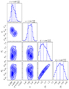 |
Fig. 1. Posterior distributions of the |

Eventually, we computed the median of the resulting posterior distribution, and the 16th and 84th percentiles intervals as associated uncertainties.
Up to this point, the model does not include the stochastic noise term, and the predicted P(k) suffers from a lack of power toward small scales with respect to the reference P(k) (see Sect. 5.4 for details). Therefore, the model parameters determined thus far correspond to the nonlocal FGPA without stochasticity. As described in Sect. 4.5, we included a further additive noise term, exclusively in voids, randomly sampled from a negative binomial distribution. To determine the best parameters for the binomial distribution θ′={fϵ, n, p}, we first manually varied the parameters until we reached a combination of θ′ that enhances the small-scale power enough and provides a good fit of the power spectrum. (see Sect. 5.4 for details). Eventually, we refit the parameters altogether, including the random component and using as an initial guess the optimal parameter values previously found. Furthermore, we adopted the following upper and lower bounds as priors on θ′: 1 < fϵ < 2, 0 < n < 1, 0 < p < 1.
We report the final estimated parameter values and their uncertainty in Table 2. We find clear differences in the best-fitting values of the same parameter in different cosmic web environments. This supports our finding that including nonlocal terms is playing an informative role in the model about missing physical dependencies in the standard FGPA.
As a final note, we stress that only the fit of parameters for the negative binomial distribution governing the random sampling of the stochastic term was determined by considering deviations between the reference and predicted power spectrum. In fact, in the fit of the parameters of the nonlocal FGPA prescription, only the PDFs were taken into account. In this sense, the fact that this bias model reproduces the power spectrum and the bispectrum with such good accuracy constitutes a reassuring sanity check.
5.2. Visual inspection of slices through the simulation box
Figure 2 shows a comparison of slices through the simulation box, obtained by averaging two contiguous slices 1.95 h−1 Mpc thick parallel to the (x, z) plane, displaying redshift space distortions along the z axis. A visual inspection between the prediction from the standard FGPA (bottom right) and the reference cosmological simulation (top left) immediately reveals that the former fails to adequately render the redshift space cosmic structures, displaying less pronounced redshift space distortions. When introducing a velocity bias correction to the standard FGPA (bottom left), redshift space distortions appear to model more appropriately the observed elongation of structures in the cosmic web; however, it turns out not to capture the saturation at F ∼ 1 in the underdense regions, which is also reflected in the probability distribution function (see also Fig. 3). We again stress that the free parameters for the FGPA model have been chosen in this case in order to match the large-scale amplitude of the power spectrum. It would also be possible to find the parameters that best fit the PDF, but this yields a severe bias (≳30%) in the large-scale predicted power spectrum amplitude. Eventually, our nonlocal FGPA model10 (top right) visually resembles the reference simulation to a good degree of approximation. In particular, it succeeds both in reproducing the redshift space structure of the cosmic web and in properly predicting the right values of flux in all the different density regimes. Without the stochasticity, underdense regions in our predicted flux would appear emptier than they actually are. This aspect is reflected in a lack of power toward small scales, as will be commented on in more detail in Sect. 5.4. The addition of the noise term, ϵ, only in voids, is meant to compensate for the lack of substructures. Therefore, we do not expect those small-scale structures to visually match the reference simulation in position. Rather, in a global sense, with the addition of the noise term, voids appear to be more filled with substructures than in the case in which we do not model stochasticity.
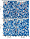 |
Fig. 2. Slices through the simulation box, obtained by averaging two contiguous slices 1.95 h−1 Mpc thick parallel to the (x, z) plane, displaying redshift space distortions along the z axis. The plot displays a Lyα forest transmitted flux F/Fc slice through the reference cosmological hydrodynamic simulation (top left), and through the predicted Lyα forest boxes obtained through the standard FGPA (bottom right), a FGPA with a velocity and threshold bias (bottom left), and our final nonlocal cosmic-web-dependent FGPA and stochasticity (top right). The maps are color-coded from red to blue for values ranging in the interval [0.1], where red indicates underdense regions and blue overdense ones. All the slices share the same color scale and the same extrema. |
5.3. Probability distribution function
Figure 3 shows a comparison between the Lyα forest PDF from the reference simulation (solid red line) and the prediction from a standard FGPA (dashed yellow line), from an FGPA with velocity bias (dotted purple line), from an FGPA with velocity and threshold bias (dash-dotted black line), and from our nonlocal FGPA with and without the addition of stochastic fluctuations in voids (dash-dotted blue and dashed green lines, respectively).
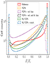 |
Fig. 3. Comparison between probability distribution functions of transmitted Lyα forest flux F/Fc as extracted from the reference simulation (red solid), and as predicted by the standard FGPA (yellow dashed), by the FGPA with velocity bias (purple dotted), by the FGPA with velocity and threshold bias (black dashed-dotted), by the nonlocal FGPA(green dashed), and by the nonlocal FGPA and stochasticity (blue dashed-dotted). |
The sharp bimodality of the Lyα forest PDF makes it particularly non-trivial to correctly predict both flux regimes, yielding the correct shape and average flux. While the standard FGPA model fails to reproduce the height of both peaks, the FGPAs with velocity (and threshold) bias prescriptions achieve a better prediction toward F ∼ 0, but a worse result at F ∼ 1, as was already commented on in Sect. 5.2. In particular, the FGPA model with threshold bias achieves a better prediction of the PDF with respect to the FGPA model with only velocity bias, but neither of the two is able to properly account for the low-density peak. The nonlocal FGPA, however, succeeds in reproducing both peaks, and qualitatively also achieves the best result among the studied cases in the intermediate flux regime, 0.1 ≲ F ≲ 0.9.
We stress that our final model, including stochasticity, with model parameters fitted to reproduce the PDFs of knots, filaments, sheets, and voids separately, yields a predicted average flux of  , in great agreement with the value from the simulation,
  , even though the model has not been explicitly calibrated to reproduce such a quantity.
We point the reader’s attention to the fact that the difference between the nonlocal FGPA (dashed green line) and the FGPA model with velocity and threshold bias (dash-dotted black line) consists in making the model sensitive to nonlocal terms. It turns out to be clear that the nonlocal dependencies play an important role in improving the prediction of the Lyα forest PDF.
5.4. Power spectrum and cross-correlation
In Fig. 4 we present a comparison between Lyα forest 3D power spectra, P(k), in the top panel, power spectrum ratios, Pmock(k)/Pref(k), in the mid panel, and cross-correlation coefficients, C(k), in the bottom panel. We display the reference simulation summary statistics as a solid red line, while we plot the predicted Lyα forest flux summary statistics as a dashed yellow line in the case of the standard FGPA, as a dotted purple line in the case of the FGPA with velocity bias, as a dash-dotted black line in the case of the FGPA with velocity and threshold bias, as a dashed green line in the case of nonlocal FGPA, and as a dash-dotted blue line the nonlocal FGPA with stochasticity. The top and bottom panels clearly highlight that the standard FGPA (dashed yellow line) and its augmented versions including velocity bias (dotted purple line) and velocity and threshold bias (dash-dotted black line) rapidly lose power toward small scales, reaching ratios Pmock(k)/Pref(k) < 20%, Pmock(k)/Pref(k) < 50%, and Pmock(k)/Pref(k) < 60%, respectively, at the Nyquist frequency knyq ∼ 1.6 h Mpc−1. As already anticipated, the P(k) predicted by the nonlocal FGPA (dashed green line) suffers from a ∼20% lack of power toward small scales with respect to the reference P(k). Eventually, the P(k) yielded by the nonlocal FGPA model with stochasticity ensures a good fit of the target power spectrum, featuring a maximum deviation of ∼3% and average deviations of ∼0.1% up to k ∼ 0.4 h Mpc−1, a maximum deviation of ∼5% and average deviations of ∼1.8% up to k ∼ 1.4 h Mpc−1, and a maximum deviation of ∼8% and average deviations of ∼0.8% up to the Nyquist frequency k ∼ 1.6 h Mpc−1.
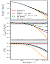 |
Fig. 4. Top: comparison of the 3D Lyα forest power spectrum, P(k). Middle: comparison of the 3D Lyα forest power spectrum ratios, Pmock(k)/Pref(k), between the predicted and reference power spectra. Bottom: comparison of cross-correlation coefficients, C(k), between the reference Lyα forest and the predictions from the different tested models. In each panel, the investigated reference simulation summary statistics are shown as a solid red line, while the prediction by the standard FGPA is displayed as a dashed yellow line, the FGPA with velocity bias as a dotted purple line, the FGPA with velocity and threshold bias as a dash-dotted black line, the nonlocal FGPA as a dashed green line, and the nonlocal FGPA with stochasticity as a dash-dotted blue line. In the mid panel, the gray shaded areas stand for 1%,2%,5%, and 10% deviations, from darker to lighter. In the bottom panel, the gray shaded areas stand for 5% and 10% deviations, from darker to lighter. |
An inspection of the bottom panel of Fig. 4, instead, reveals that the standard FGPA (dashed yellow line) delivers a lower C(k) with respect to all the other cases that incorporate the modeling of velocity bias. In fact, looking at Fig. 2, it can be appreciated by eye how the standard FGPA (top right) does not model properly the enhancement of cosmic structure elongation along the line of sight clearly seen in the reference simulation (top left). In this sense, an adequate treatment of velocity bias ensures a better cross-correlation at all scales. The nonlocal FGPA (dashed green line) displays a larger C(k) than the standard FGPA (dashed yellow line) than the local FGPA with velocity bias (dotted purple line) and than the local FGPA with velocity bias (dotted purple line) at all scales, from a 1% gain in C(k) on large scales up to a ∼3% gain in C(k) at k ∼ 1.0 h Mpc−1. Eventually, the nonlocal FGPA with stochasticity (dash-dotted blue line) features a slightly lower C(k) than the nonlocal FGPA (dashed green line) up to k ∼ 0.5 h Mpc−1, while it starts to depart from the latter at larger k, lacking a ∼6% C(k) at k ∼ 1.0 h Mpc−1. This is expected by construction, due to the addition of a random component, which has the effect of lowering the cross-correlation. However, the loss of C(k) is not dramatic, and the nonlocal FPGA model with stochasticity (dash-dotted blue line) still improves the local FGPA with velocity bias C(k) (dotted purple line) up to k ∼ 0.8 h Mpc−1. Remarkably, the FGPA model with velocity and threshold bias is found to provide the highest C(k) across all scales, even though it is very similar to the prediction by the nonlocal FGPA model.
Here again, the difference between the nonlocal FGPA (dashed green line) and the FGPA model with velocity and threshold bias (dash-dotted black line) consists of the inclusion of the nonlocal dependence on the cosmic web. The remarkable difference (≳20% gain in the accuracy of the predicted P(k) at the Nyquist frequency) makes clear the improvement accounted for by the nonlocal model.
5.5. Bispectrum
To address the capability of the model to reproduce higher-order statistics, we also assessed the accuracy of the predicted bispectrum. We report in Fig. 5 the reduced bispectrum, Q(θ12), as a function of the subtended angle, θ12, for four different triangular configurations: (i) k1 = 0.1, k = 0.2 h Mpc−1 (top left), (ii) k1 = 0.2, k = 0.2 h Mpc−1 (top right), (iii) k1 = 0.3, k = 0.5 h Mpc−1 (bottom left), and (iv) k1 = 0.5, k = 0.5 h Mpc−1 (bottom right). The plot displays the bispectrum of the reference simulation (solid red line), compared to the predictions from the standard FGPA (dashed yellow line), the FGPA with velocity bias (dotted purple line), the FGPA with velocity and threshold bias (dash-dotted black line), the nonlocal FGPA (dashed green line), and the nonlocal FGPA with stochasticity (dash-dotted blue line). The latter (i.e., our preferred model) reproduces the target bispectrum with reasonable accuracy for all the probed triangular configurations, while the others start to feature significant deviations at k ≳ 0.2 h Mpc−1. In particular, the nonlocal FGPA model with stochasticity reproduces not only the overall shape of the reference bispectrum, but also some peculiar features, such as the position and amplitude of the peak around θ ∼ 2.3 in the k1 = k2 = 0.5 h Mpc−1 configuration, as well as the position (although not very much the amplitude) of the peak around θ ∼ 2.1 in the k1 = 0.3, k2 = 0.5 h Mpc−1 configuration.
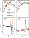 |
Fig. 5. Reduced bispectrum, Q(θ12), as a function of the subtended angle, θ12, for four different triangular configurations: (i) k1 = 0.1, k = 0.2 h Mpc−1 (top left), (ii) k1 = 0.2, k = 0.2 h Mpc−1 (top right), (iii) k1 = 0.3, k = 0.5 h Mpc−1 (bottom left), and (iv) k1 = 0.5, k = 0.5 h Mpc−1 (bottom right). The plot displays the bispectrum of the reference simulation (solid red line), compared to the predictions from the standard FGPA (dashed yellow line), the FGPA with velocity bias (dotted purple line), the FGPA with velocity and threshold bias (dash-dotted black line), the nonlocal FGPA (dashed green line), and the nonlocal FGPA with stochasticity (dash-dotted blue line). The latter (i.e., our preferred model) reproduces the target bispectrum with reasonable accuracy for all the probed triangular configurations, while the others start to feature significant deviations at k ≳ 0.2 h Mpc−1. |
6. Lightcone generation
In this section we illustrate how our method can be generalized to other redshifts and applied to generate Lyα forest lightcones.
We start by noticing that we have the following redshifts available from the simulation: z = 1.8, 2.0, 2.2, 2.4, 2.6, 2.8, 3.0, and 4.0.
First, we show that the method also generalizes at other redshifts. To do so, we re-calibrated the parameters of our model at z = 1.8 and 2.2. Figure 6 shows the resulting Lyα forest power spectra ratios at z = 1.8 (dotted purple line) and at z = 2.2 (dashed green line). The achieved accuracy is very similar to that shown in Fig. 4 (mid panel) at z = 2. Subsequently we demonstrate that, once the calibration is performed for some redshift snapshots, we can interpolate the parameters for the redshifts in between and ensure a continuous smooth redshift evolution. In particular, we linearly interpolated the parameters obtained at z = 1.8 and z = 2.2 and predicted the Lyα forest field at z = 2. We show the resulting P(k) at z = 2 in Fig. 6 (dash-dotted blue line), noticing that again the achieved accuracy is very similar to the one we get via direct calibration at z = 2.
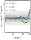 |
Fig. 6. Comparison of 3D Lyα forest power spectrum ratios, Pmock(k)/Pref(k), between the predicted and reference power spectra at different redshifts. Results at z = 1.8 (dotted purple line) and z = 2.2 (dashed green line) are obtained via independent calibrations. Instead, the z = 2 result (dash-dotted blue line) corresponds to the Lyα forest power spectrum that we get by applying the nonlocal FGPA model with parameters linearly interpolated at z = 2 from calibrations at z = 1.8 and z = 2.2. The gray shaded areas stand for 1%,2%,5%, and 10% deviations, from darker to lighter. |
Afterward, we also re-calibrated the model parameters for the remaining redshift snapshots and generated a lightcone box as follows. We considered the redshift range Δz = [1.8, 3.8]. The comoving radial distance subtended by this redshift interval is l ∼ 1500 h−1 Mpc. Therefore, after having mapped the dark matter fields at all redshift from real to redshift space, we replicated the same simulation box three times in the redshift direction. Then, we connected the redshift space dark matter field snapshots transitioning from one to the following at the average redshift between the two. Even though this implies a sharp transition in the dark matter field, we painted the Lyα forest on the lightcone by interpolating the parameters of the model with a cubic spline interpolation scheme at each redshift slice. This ensured a smooth redshift evolution. We show a slice through the final lightcone box in Fig. 7. One can clearly visualize how the Lyα forest changes from z = 1.8 to z = 3.8, with voids becoming bigger and emptier toward the low-redshift end.
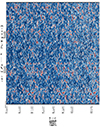 |
Fig. 7. Slice through the lightcone box with redshift evolution from z = 1.8 to z = 3.8. The lightcone was obtained by replicating three times the same simulation box in the redshift direction and connecting the different redshift space dark matter field snapshots. Afterward, the Lyα forest was painted on the dark matter lightcone by interpolating the parameters of the model calibrated at different redshift snapshots, as illustrated in Sect. 6. One can visually appreciate the redshift evolution, with voids becoming bigger and emptier toward the low-redshift end. |
In a forthcoming publication, we will present full-sky Lyα forest mocks by generating dark matter fields with lightcone geometry and smooth evolution in redshift already in the dark matter field (Sinigaglia et al., in prep.).
7. Potential future improvements
While the presented model, as anticipated, turns out to be sufficient to fulfill the purpose it was designed for, there are further potential improvements that we leave to be explored in future works.
In this work, we include nonlocal dependencies in the bias formulation only through the T-web. Such dependencies are known to have a long-range effect (e.g., McDonald & Roy 2009), and we are hence neglecting short-range terms, the effect of which kicks in when it comes to modeling the nonlinear clustering toward small scales. Short-range nonlocal terms can be constructed as scalars from the curvature tensor δij = ∂i∂jδ, such as its Laplacian ∇2δ in Eulerian (e.g., Peacock & Heavens 1985; McDonald & Roy 2009; Werner & Porciani 2020; Kitaura et al. 2022) or Lagrangian space (e.g., Zennaro et al. 2022), which characterizes the shape of the local maxima of the density field (Peacock & Heavens 1985). More generally, one can build short-range nonlocal terms as scalars computed from arbitrarily higher-order derivatives of the density field, such as  (e.g., Kitaura et al. 2022). Alternatively, in analogy with the I-web description based on the invariants of the tidal field tensor (see also Sect. 3), one can work in a framework relying on the invariants of the curvature tensor. This latter description has been proven to encode crucial information to model the bias of baryon density fields (e.g., Sinigaglia et al. 2021, 2022). Since we do not model such a family of dependencies here, we stress that we may be missing some relevant piece of physical information. However, we also stress that computing such terms requires an accurate enough modeling of small scales, which is not guaranteed here. Therefore, by introducing short-range nonlocal terms we may face the risk of introducing a noisy component, to the detriment of the final accuracy. Moreover, in the computationally cheapest way of modeling such dependencies, we would be extracting the analogous to the T-web based on δij, which would imply a non-negligible number of additional free parameters in our model.
In connection to the previous point, we note that Kitaura et al. (2022) show that the I-web model encodes a larger amount of information on the clustering of biased tracers with respect to the T-web, at the expense of a larger number of parameters (the number of bins used to described the invariants), and therefore is at a greater risk of incurring overfitting. Moreover, while describing the nonlocal quantities by explicitly using the invariants of the tidal tensor is possible (e.g., Pellejero-Ibañez et al. 2020), it implies devising a suitable functional form for each additional term used in the bias, which is in principle nontrivial.
Another point that can be improved consists of the way we modeled the low-density regions, identified as cosmic voids according to the T-web classification. In fact, in order to compensate for the lack of substructures, we randomly sampled a noise component from a negative binomial distribution. At this point we noticed that this could be avoided, or its impact alleviated, by improving the modeling of the deterministic component. One easy modification could consist of binning the density distribution in voids into an arbitrary number of intervals, and identifying distinct parameters for such distinct density bins. However, this would again introduce a larger number of free parameters in our model.
Eventually, if a noise term is to be included as is done in this work, we note that we have randomly sampled the stochastic component from a negative binomial distribution, for the reasons previously stated, but this is not the only possible solution. In fact, one may find that using a different distribution may be more convenient.
We leave all these potential improvements to be investigated in future publications, or in applications adopting this model.
8. Conclusions
This work presents a significantly augmented version of the widely used FGPA to predict the Lyα forest in redshift space, as observed from current and forthcoming spectroscopic galaxy surveys. This new model relies on explicit modeling of velocity bias and redshift space distortions and of a modification to the FGPA introducing a cutoff and a boosting scale, with free parameters (determined based on both heuristic and physical arguments, as well as on an efficient MCMC scheme) made dependent on the cosmic web environment as described by the T-web classification (knots, filaments, sheets, and voids, Hahn et al. 2007). In this sense, we label our model a “nonlocal” FGPA. In fact, the Lyα forest flux in each cell is here made dependent on the content of the surrounding cells and the geometry of the gravitational field, and the model effectively incorporates nonlocal bias information up to third-order in Eulerian perturbative bias expansion (see Kitaura et al. 2022). In addition, since we find that such a model fails to reproduce the small-scale clustering in the underdense regions, we add a further stochastic term only in voids, randomly sampled from a negative binomial distribution. This random component has the effect of enhancing the small-scale power, and hence of improving the fit of the Lyα forest forest 3D power spectrum toward small scales.
We predicted Lyα forest fluxes with a standard FGPA, our preferred nonlocal FGPA model with stochasticity, and three other intermediate models in between, on a mesh with V = (500 h−1 Mpc)3 volume and Nc = 2563 cells, with physical cell resolution l ∼ 1.95 h−1 Mpc, trying to reproduce a full cosmological hydrodynamic N-body/SPH simulation (spanning the same volume) and run with N = 10243 particles. We assessed the accuracy of the prediction of such models by comparing the results regarding the mean transmitted flux,  , the PDF, the power spectrum, and the bispectrum, with the analogous summary statistics computed from the reference simulation.
The augmented nonlocal FGPA with stochasticity improves upon the standard FGPA model in all the investigated summary statistics. In fact, the nonlocal FGPA accurately reproduces the mean transmitted flux,  , the flux PDF, the power spectrum, and the bispectrum. In particular, our model yields a mean transmitted flux,
  , in excellent agreement with the value
  , and a power spectrum featuring a maximum deviation of ∼3% and average deviations of ∼0.1% up to k ∼ 0.4 h Mpc−1, a maximum deviation of ∼5% and average deviations of ∼1.8% up to k ∼ 1.4 h Mpc−1, and a maximum deviation of ∼8% and average deviations of ∼0.8% up to the Nyquist frequency k ∼ 1.6 h Mpc−1. The predicted PDF and the bispectrum clearly outperform the results from any other model tested in this paper as well.
Compared to other schemes based on machine learning (e.g., Harrington et al. 2022; Horowitz et al. 2022a; Sinigaglia et al. 2022) and other methods based on iterative calibrations (e.g., Sorini et al. 2016; Peirani et al. 2022), our model has the appeal of being a purely analytical method, and therefore it is fast to compute, less prone to the overfitting problem, and can be straightforwardly generalized to larger or smaller volumes, different mesh resolutions, and at different redshift snapshots. This method can even ensure a continuous smooth treatment of redshift evolution via interpolation of the fitting coefficients in between the redshift snapshots used for calibration, avoiding discontinuity problems at the edge of distinct contiguous redshift shells.
We point out that the resolution (1.95 h−1 Mpc physical cell size) considered in this work is not sufficient to provide realistic Lyα forest high-resolution spectra with correct modeling of the 1D power spectrum, needed to perform studies of small-scale (k ∼ 5 − 10 h Mpc−1) physics, such as bounds on the mass of warm dark matter particles (Viel et al. 2005, 2013) and of neutrinos (Palanque-Delabrouille et al. 2015) and constraints on the thermal state of the intergalactic medium (Garzilli et al. 2017, and references therein), among others. While the application of the nonlocal FGPA to high-resolution density fields is possible, one should bear in mind that resolving sub-Mpc scales on a 3D mesh makes it computationally very expensive to realize large-volume cosmological boxes. Therefore, in future works, we will explore novel techniques based on Bayesian inference aimed at upsampling the resolution of 1D Lyα forest skewers extracted from low-resolution Lyα forest flux boxes generated following the procedure presented in this work.
We plan to adopt this novel scheme to generate Lyα forest mock lightcones for the DESI survey, in combination with accurate approximated gravity solvers correcting for shell-crossing (e.g., Kitaura & Hess 2013; Tosone et al. 2021; Kitaura et al. 2023). In particular, we aim to use a recent fast structure formation model based on iterative Eulerian Lagrangian perturbation theory (eALPT, Kitaura et al. 2023), which has been shown to reproduce the clustering of N-body simulations with percent accuracy deep into the nonlinear regime. Furthermore, the application of the nonlocal FGPA model to approximated dark matter fields generated through the ALPT or eALPT approximations can potentially represent a new avenue in Bayesian density field reconstruction studies using the Lyα forest. We will investigate this point in future publications.
In conclusion, we argue that this novel nonlocal FGPA scheme represents a significant step forward with respect to previous analytical efforts, and could become instrumental in the generation of fast accurate mocks for covariance matrices estimation in the context of current and forthcoming Lyα forest surveys.
The code implementing the model presented in this work has been made publicly available11.
SKAO: https://www.skao.int
ELT: https://elt.eso.org
Artificial Intelligence.
The notation F = exp(−τ) for the Lyα forest flux field actually refers to the transmitted flux F/Fc, in other words to the quasar spectrum normalized to its continuum Fc. We will omit hereafter the normalization and denote the transmitted flux just as F unless specified otherwise.
We adopt the nomenclature “standard” in contrast to the nonlocal FGPA version presented in the following sections.
We hereafter adopt the following subscript notation: kn = knots, fl = filaments, sh = sheets, vd = voids.
While other parameterizations are possible, we stick to the one used in this work and reported in the numpy (Harris et al. 2020) documentation, for the sake of the reproducibility of results.
n is in principle an integer number, but its definition can be generalized to reals, as is done in this work.
We hereafter omit to write that the nonlocal model also includes velocity and threshold bias.
Acknowledgments
The authors wish to warmly thank the anonymous referee for the insightful comments they provided, which helped to improve the quality of the manuscript. We are grateful to Cheng Zhao for making his bispectrum computation code available. F.S. acknowledges the support of the doctoral grant funded by the University of Padova and by the Italian Ministry of Education, University and Research (MIUR) and the financial support of the Fondazione Ing. Aldo Gini fellowship. F.S. is indebted to the Instituto de Astrofísica de Canarias (IAC) for hospitality and the availability of computing resources during the realization of this project. F.S.K. and A.B.A acknowledge the IAC facilities and the Spanish Ministry of Science and Innovation (MICIN) under the Big Data of the Cosmic Web project PID2020-120612GB-I00. K.N. is grateful to Volker Springel for providing the original version of GADGET-3, on which the GADGET3-OSAKA code is based. Our numerical simulations and analyses were carried out on the XC50 systems at the Center for Computational Astrophysics (CfCA) of the National Astronomical Observatory of Japan (NAOJ), the Yukawa-21 at YITP in Kyoto University, SQUID at the Cybermedia Center, Osaka University as part of the HPCI system Research Project (hp210090). This work is supported in part by the JSPS KAKENHI Grant Number JP17H01111, 19H05810, 20H00180 (K.N.), 21J20930, 22KJ2072 (Y.O.). K.N. acknowledges the travel support from the Kavli IPMU, World Premier Research Center Initiative (WPI), where part of this work was conducted.
References
- Amendola, L., Appleby, S., Avgoustidis, A., et al. 2018, Liv. Rev. Relat., 21, 2 [Google Scholar]
- Ando, R., Nishizawa, A. J., Hasegawa, K., Shimizu, I., & Nagamine, K. 2019, MNRAS, 484, 5389 [NASA ADS] [CrossRef] [Google Scholar]
- Aoyama, S., Hou, K.-C., Hirashita, H., Nagamine, K., & Shimizu, I. 2018, MNRAS, 478, 4905 [NASA ADS] [CrossRef] [Google Scholar]
- Balaguera-Antolínez, A., Kitaura, F.-S., Pellejero-Ibáñez, M., Zhao, C., & Abel, T. 2018, MNRAS, 483, L58 [Google Scholar]
- Balaguera-Antolínez, A., Kitaura, F.-S., Pellejero-Ibáñez, M., et al. 2019, MNRAS, 491, 2565 [Google Scholar]
- Balaguera-Antolínez, A., Kitaura, F.-S., Alam, S., et al. 2023, A&A, 673, A130 [NASA ADS] [CrossRef] [EDP Sciences] [Google Scholar]
- Bardeen, J. M., Bond, J. R., Kaiser, N., & Szalay, A. S. 1986, ApJ, 304, 15 [Google Scholar]
- Bond, J. R., Kofman, L., & Pogosyan, D. 1996, Nature, 380, 603 [NASA ADS] [CrossRef] [Google Scholar]
- Cautun, M., van de Weygaert, R., Jones, B. J. T., & Frenk, C. S. 2014, MNRAS, 441, 2923 [Google Scholar]
- Cieplak, A. M., & Slosar, A. 2016, J. Cosmol. Astropart. Phys., 2016, 016 [CrossRef] [Google Scholar]
- Croft, R. A. C., Weinberg, D. H., Katz, N., & Hernquist, L. 1998, in Large Scale Structure: Tracks and Traces, eds. V. Mueller, S. Gottloeber, J. P. Muecket, & J. Wambsganss, 69 [Google Scholar]
- du Mas des Bourboux, H., Rich, J., Font-Ribera, A., et al. 2020, ApJ, 901, 153 [CrossRef] [Google Scholar]
- Eisenstein, D. J., Seo, H.-J., Sirko, E., & Spergel, D. N. 2007, ApJ, 664, 675 [NASA ADS] [CrossRef] [Google Scholar]
- Farr, J., Font-Ribera, A., du Mas des Bourboux, H., et al. 2020, J. Cosmol. Astropart. Phys., 2020, 068 [CrossRef] [Google Scholar]
- Font-Ribera, A., McDonald, P., & Miralda-Escudé, J. 2012, J. Cosmol. Astropart. Phys., 2012, 001 [CrossRef] [Google Scholar]
- Foreman-Mackey, D., Hogg, D. W., Lang, D., & Goodman, J. 2013, PASP, 125, 306 [Google Scholar]
- Forero-Romero, J. E., Hoffman, Y., Gottlöber, S., Klypin, A., & Yepes, G. 2009, MNRAS, 396, 1815 [Google Scholar]
- Garzilli, A., Boyarsky, A., & Ruchayskiy, O. 2017, Phys. Lett. B, 773, 258 [NASA ADS] [CrossRef] [Google Scholar]
- Goodman, J., & Weare, J. 2010, Commun. Appl. Math. Comput. Sci., 5, 65 [Google Scholar]
- Greene, J., Bezanson, R., Ouchi, M., Silverman, J., & the PFS Galaxy Evolution Working Group 2022, ArXiv e-prints [arXiv:2206.14908] [Google Scholar]
- Haardt, F., & Madau, P. 2012, ApJ, 746, 125 [Google Scholar]
- Hahn, O., Porciani, C., Carollo, C. M., & Dekel, A. 2007, MNRAS, 375, 489 [NASA ADS] [CrossRef] [Google Scholar]
- Hahn, O., Rampf, C., & Uhlemann, C. 2021, MNRAS, 503, 426 [NASA ADS] [CrossRef] [Google Scholar]
- Hamilton, A. J. S. 1998, in Linear Redshift Distortions: a Review, ed. D. Hamilton, 231, 185 [Google Scholar]
- Harrington, P., Mustafa, M., Dornfest, M., Horowitz, B., & Lukić, Z. 2022, ApJ, 929, 160 [NASA ADS] [CrossRef] [Google Scholar]
- Harris, C. R., Millman, K. J., van der Walt, S. J., et al. 2020, Nature, 585, 357 [NASA ADS] [CrossRef] [Google Scholar]
- Heß, S., Kitaura, F.-S., & Gottlöber, S. 2013, MNRAS, 435, 2065 [CrossRef] [Google Scholar]
- Hockney, R. W., & Eastwood, J. W. 1981, Computer Simulation Using Particles (Boca Raton: CRC Press) [Google Scholar]
- Hopkins, P. F., Narayanan, D., Murray, N., & Quataert, E. 2013, MNRAS, 433, 69 [NASA ADS] [CrossRef] [Google Scholar]
- Horowitz, B., Lee, K.-G., White, M., Krolewski, A., & Ata, M. 2019, ApJ, 887, 61 [NASA ADS] [CrossRef] [Google Scholar]
- Horowitz, B., Dornfest, M., Lukić, Z., & Harrington, P. 2022a, ApJ, 941, 42 [NASA ADS] [CrossRef] [Google Scholar]
- Horowitz, B., Lee, K.-G., Ata, M., et al. 2022b, ApJS, 263, 27 [NASA ADS] [CrossRef] [Google Scholar]
- Hui, L., & Gnedin, N. Y. 1997, MNRAS, 292, 27 [Google Scholar]
- Kaiser, N. 1984, ApJ, 284, L9 [NASA ADS] [CrossRef] [Google Scholar]
- Kaiser, N. 1987, MNRAS, 227, 1 [Google Scholar]
- Kitaura, F. S., & Hess, S. 2013, MNRAS, 435, L78 [NASA ADS] [CrossRef] [Google Scholar]
- Kitaura, F. S., Yepes, G., & Prada, F. 2014, MNRAS, 439, L21 [NASA ADS] [CrossRef] [Google Scholar]
- Kitaura, F.-S., Gil-Marín, H., Scóccola, C. G., et al. 2015, MNRAS, 450, 1836 [NASA ADS] [CrossRef] [Google Scholar]
- Kitaura, F.-S., Chuang, C.-H., Liang, Y., et al. 2016a, Phys. Rev. Lett., 116, 171301 [NASA ADS] [CrossRef] [Google Scholar]
- Kitaura, F.-S., Rodríguez-Torres, S., Chuang, C.-H., et al. 2016b, MNRAS, 456, 4156 [NASA ADS] [CrossRef] [Google Scholar]
- Kitaura, F. S., Balaguera-Antolínez, A., Sinigaglia, F., & Pellejero-Ibáñez, M. 2022, MNRAS, 512, 2245 [NASA ADS] [CrossRef] [Google Scholar]
- Kitaura, F.-S., Sinigaglia, F., Balaguera-Antolínez, A., & Favole, G. 2023, ArXiv e-prints [arXiv:2301.03648] [Google Scholar]
- Kooistra, R., Lee, K.-G., & Horowitz, B. 2022, ApJ, 938, 123 [NASA ADS] [CrossRef] [Google Scholar]
- Krolewski, A., Lee, K.-G., Lukić, Z., & White, M. 2017, ApJ, 837, 31 [NASA ADS] [CrossRef] [Google Scholar]
- Lee, K.-G., & White, M. 2016, ApJ, 831, 181 [NASA ADS] [CrossRef] [Google Scholar]
- Lee, K.-G., Hennawi, J. F., White, M., Croft, R. A. C., & Ozbek, M. 2014, ApJ, 788, 49 [NASA ADS] [CrossRef] [Google Scholar]
- Lee, K.-G., Krolewski, A., White, M., et al. 2018, ApJS, 237, 31 [Google Scholar]
- Le Goff, J. M., Magneville, C., Rollinde, E., et al. 2011, A&A, 534, A135 [NASA ADS] [CrossRef] [EDP Sciences] [Google Scholar]
- Levi, M., Bebek, C., Beers, T., et al. 2013, ArXiv e-prints [arXiv:1308.0847] [Google Scholar]
- Libeskind, N. I., van de Weygaert, R., Cautun, M., et al. 2017, MNRAS, 473, 1195 [Google Scholar]
- Lukić, Z., Stark, C. W., Nugent, P., et al. 2015, MNRAS, 446, 3697 [CrossRef] [Google Scholar]
- Martizzi, D., Vogelsberger, M., Artale, M. C., et al. 2019, MNRAS, 486, 3766 [Google Scholar]
- McDonald, P., & Roy, A. 2009, J. Cosmol. Astropart. Phys., 2009, 020 [CrossRef] [Google Scholar]
- Meiksin, A., & White, M. 2001, MNRAS, 324, 141 [CrossRef] [Google Scholar]
- Mo, H. J., & White, S. D. M. 2002, MNRAS, 336, 112 [Google Scholar]
- Momose, R., Shimizu, I., Nagamine, K., et al. 2021, ApJ, 911, 98 [NASA ADS] [CrossRef] [Google Scholar]
- Nagamine, K., Shimizu, I., Fujita, K., et al. 2021, ApJ, 914, 66 [NASA ADS] [CrossRef] [Google Scholar]
- Newman, A. B., Rudie, G. C., Blanc, G. A., et al. 2020, ApJ, 891, 147 [NASA ADS] [CrossRef] [Google Scholar]
- Neyrinck, M. C., Aragón-Calvo, M. A., Jeong, D., & Wang, X. 2014, MNRAS, 441, 646 [Google Scholar]
- Palanque-Delabrouille, N., Yèche, C., Baur, J., et al. 2015, J. Cosmol. Astropart. Phys., 2015, 011 [CrossRef] [Google Scholar]
- Peacock, J. A., & Heavens, A. F. 1985, MNRAS, 217, 805 [NASA ADS] [CrossRef] [Google Scholar]
- Peebles, P. J. E. 1980, The Large-scale Structure of the Universe (Princeton: Princeton University Press) [Google Scholar]
- Peirani, S., Weinberg, D. H., Colombi, S., et al. 2014, ApJ, 784, 11 [NASA ADS] [CrossRef] [Google Scholar]
- Peirani, S., Prunet, S., Colombi, S., et al. 2022, MNRAS, 514, 3222 [NASA ADS] [CrossRef] [Google Scholar]
- Pellejero-Ibañez, M., Balaguera-Antolínez, A., Kitaura, F.-S., et al. 2020, MNRAS, 493, 586 [CrossRef] [Google Scholar]
- Pieri, M. M., Bonoli, S., Chaves-Montero, J., et al. 2016, in SF2A-2016: Proceedings of the Annual meeting of the French Society of Astronomy and Astrophysics, eds. C. Reylé, J. Richard, L. Cambrésy, et al., 259 [Google Scholar]
- Planck Collaboration VI. 2020, A&A, 641, A6 [NASA ADS] [CrossRef] [EDP Sciences] [Google Scholar]
- Porqueres, N., Hahn, O., Jasche, J., & Lavaux, G. 2020, A&A, 642, A139 [NASA ADS] [CrossRef] [EDP Sciences] [Google Scholar]
- Rauch, M. 1998, ARA&A, 36, 267 [Google Scholar]
- Rorai, A., Hennawi, J. F., & White, M. 2013, ApJ, 775, 81 [NASA ADS] [CrossRef] [Google Scholar]
- Saitoh, T. R. 2017, AJ, 153, 85 [NASA ADS] [CrossRef] [Google Scholar]
- Saitoh, T. R., & Makino, J. 2009, ApJ, 697, L99 [NASA ADS] [CrossRef] [Google Scholar]
- Saitoh, T. R., & Makino, J. 2013, ApJ, 768, 44 [NASA ADS] [CrossRef] [Google Scholar]
- Seljak, U. 2012, J. Cosmol. Astropart. Phys., 2012, 004 [Google Scholar]
- Sheth, R. K., Mo, H. J., & Tormen, G. 2001, MNRAS, 323, 1 [NASA ADS] [CrossRef] [Google Scholar]
- Shimizu, I., Todoroki, K., Yajima, H., & Nagamine, K. 2019, MNRAS, 484, 2632 [NASA ADS] [CrossRef] [Google Scholar]
- Sinigaglia, F., Kitaura, F.-S., Balaguera-Antolínez, A., et al. 2021, ApJ, 921, 66 [NASA ADS] [CrossRef] [Google Scholar]
- Sinigaglia, F., Kitaura, F.-S., Balaguera-Antolínez, A., et al. 2022, ApJ, 927, 230 [NASA ADS] [CrossRef] [Google Scholar]
- Slosar, A., Ho, S., White, M., & Louis, T. 2009, J. Cosmol. Astropart. Phys., 2009, 019 [NASA ADS] [CrossRef] [Google Scholar]
- Smith, B. D., Bryan, G. L., Glover, S. C. O., et al. 2017, MNRAS, 466, 2217 [NASA ADS] [CrossRef] [Google Scholar]
- Sorini, D., Oñorbe, J., Lukić, Z., & Hennawi, J. F. 2016, ApJ, 827, 97 [NASA ADS] [CrossRef] [Google Scholar]
- Springel, V. 2005, MNRAS, 364, 1105 [Google Scholar]
- Takada, M., Ellis, R. S., Chiba, M., et al. 2014, PASJ, 66, R1 [Google Scholar]
- Tasitsiomi, A. 2006, ApJ, 645, 792 [NASA ADS] [CrossRef] [Google Scholar]
- Tosone, F., Neyrinck, M. C., Granett, B. R., Guzzo, L., & Vittorio, N. 2021, MNRAS, 505, 2999 [NASA ADS] [CrossRef] [Google Scholar]
- Vakili, M., Kitaura, F.-S., Feng, Y., et al. 2017, MNRAS, 472, 4144 [CrossRef] [Google Scholar]
- Viel, M., Matarrese, S., Mo, H. J., Theuns, T., & Haehnelt, M. G. 2002, MNRAS, 336, 685 [CrossRef] [Google Scholar]
- Viel, M., Lesgourgues, J., Haehnelt, M. G., Matarrese, S., & Riotto, A. 2005, Phys. Rev. D, 71, 063534 [NASA ADS] [CrossRef] [Google Scholar]
- Viel, M., Becker, G. D., Bolton, J. S., & Haehnelt, M. G. 2013, Phys. Rev. D, 88, 043502 [NASA ADS] [CrossRef] [Google Scholar]
- Weinberg, D., Burles, S., Croft, R. A. C., et al. 1999, in Evolution of Large Scale Structure : From Recombination to Garching, eds. A. J. Banday, R. K. Sheth, L. N. da Costa, 346 [Google Scholar]
- Werner, K. F., & Porciani, C. 2020, MNRAS, 492, 1614 [NASA ADS] [CrossRef] [Google Scholar]
- White, M., Pope, A., Carlson, J., et al. 2010, ApJ, 713, 383 [NASA ADS] [CrossRef] [Google Scholar]
- Yang, X., Zhang, Y., Lu, T., et al. 2017, ApJ, 848, 60 [NASA ADS] [CrossRef] [Google Scholar]
- Zel’dovich, Y. B. 1970, A&A, 5, 84 [NASA ADS] [Google Scholar]
- Zennaro, M., Angulo, R. E., Contreras, S., Pellejero-Ibáñez, M., & Maion, F. 2022, MNRAS, 514, 5443 [NASA ADS] [CrossRef] [Google Scholar]
- Zhao, C., Kitaura, F.-S., Chuang, C.-H., et al. 2015, MNRAS, 451, 4266 [NASA ADS] [CrossRef] [Google Scholar]
All Tables
Volume filling factors of each cosmic web type for the real space dark matter field, and the redshift space dark matter field obtained by applying the RSD description, including velocity bias dependent on the real space T-web with parameters described in the upper part of Table 2 (see Sect. 4.2 for the details about the procedure), and used to compute our final nonlocal FGPA model.
Best-fit model parameters for our preferred nonlocal FGPA prescription with stochasticity.
All Figures
|
Fig. 1. Posterior distributions of the |
| In the text | |
|
Fig. 2. Slices through the simulation box, obtained by averaging two contiguous slices 1.95 h−1 Mpc thick parallel to the (x, z) plane, displaying redshift space distortions along the z axis. The plot displays a Lyα forest transmitted flux F/Fc slice through the reference cosmological hydrodynamic simulation (top left), and through the predicted Lyα forest boxes obtained through the standard FGPA (bottom right), a FGPA with a velocity and threshold bias (bottom left), and our final nonlocal cosmic-web-dependent FGPA and stochasticity (top right). The maps are color-coded from red to blue for values ranging in the interval [0.1], where red indicates underdense regions and blue overdense ones. All the slices share the same color scale and the same extrema. |
| In the text | |
|
Fig. 3. Comparison between probability distribution functions of transmitted Lyα forest flux F/Fc as extracted from the reference simulation (red solid), and as predicted by the standard FGPA (yellow dashed), by the FGPA with velocity bias (purple dotted), by the FGPA with velocity and threshold bias (black dashed-dotted), by the nonlocal FGPA(green dashed), and by the nonlocal FGPA and stochasticity (blue dashed-dotted). |
| In the text | |
|
Fig. 4. Top: comparison of the 3D Lyα forest power spectrum, P(k). Middle: comparison of the 3D Lyα forest power spectrum ratios, Pmock(k)/Pref(k), between the predicted and reference power spectra. Bottom: comparison of cross-correlation coefficients, C(k), between the reference Lyα forest and the predictions from the different tested models. In each panel, the investigated reference simulation summary statistics are shown as a solid red line, while the prediction by the standard FGPA is displayed as a dashed yellow line, the FGPA with velocity bias as a dotted purple line, the FGPA with velocity and threshold bias as a dash-dotted black line, the nonlocal FGPA as a dashed green line, and the nonlocal FGPA with stochasticity as a dash-dotted blue line. In the mid panel, the gray shaded areas stand for 1%,2%,5%, and 10% deviations, from darker to lighter. In the bottom panel, the gray shaded areas stand for 5% and 10% deviations, from darker to lighter. |
| In the text | |
|
Fig. 5. Reduced bispectrum, Q(θ12), as a function of the subtended angle, θ12, for four different triangular configurations: (i) k1 = 0.1, k = 0.2 h Mpc−1 (top left), (ii) k1 = 0.2, k = 0.2 h Mpc−1 (top right), (iii) k1 = 0.3, k = 0.5 h Mpc−1 (bottom left), and (iv) k1 = 0.5, k = 0.5 h Mpc−1 (bottom right). The plot displays the bispectrum of the reference simulation (solid red line), compared to the predictions from the standard FGPA (dashed yellow line), the FGPA with velocity bias (dotted purple line), the FGPA with velocity and threshold bias (dash-dotted black line), the nonlocal FGPA (dashed green line), and the nonlocal FGPA with stochasticity (dash-dotted blue line). The latter (i.e., our preferred model) reproduces the target bispectrum with reasonable accuracy for all the probed triangular configurations, while the others start to feature significant deviations at k ≳ 0.2 h Mpc−1. |
| In the text | |
|
Fig. 6. Comparison of 3D Lyα forest power spectrum ratios, Pmock(k)/Pref(k), between the predicted and reference power spectra at different redshifts. Results at z = 1.8 (dotted purple line) and z = 2.2 (dashed green line) are obtained via independent calibrations. Instead, the z = 2 result (dash-dotted blue line) corresponds to the Lyα forest power spectrum that we get by applying the nonlocal FGPA model with parameters linearly interpolated at z = 2 from calibrations at z = 1.8 and z = 2.2. The gray shaded areas stand for 1%,2%,5%, and 10% deviations, from darker to lighter. |
| In the text | |
|
Fig. 7. Slice through the lightcone box with redshift evolution from z = 1.8 to z = 3.8. The lightcone was obtained by replicating three times the same simulation box in the redshift direction and connecting the different redshift space dark matter field snapshots. Afterward, the Lyα forest was painted on the dark matter lightcone by interpolating the parameters of the model calibrated at different redshift snapshots, as illustrated in Sect. 6. One can visually appreciate the redshift evolution, with voids becoming bigger and emptier toward the low-redshift end. |
| In the text | |
Current usage metrics show cumulative count of Article Views (full-text article views including HTML views, PDF and ePub downloads, according to the available data) and Abstracts Views on Vision4Press platform.
Data correspond to usage on the plateform after 2015. The current usage metrics is available 48-96 hours after online publication and is updated daily on week days.
Initial download of the metrics may take a while.