| Issue |
A&A
Volume 671, March 2023
|
|
|---|---|---|
| Article Number | L14 | |
| Number of page(s) | 7 | |
| Section | Letters to the Editor | |
| DOI | https://doi.org/10.1051/0004-6361/202346240 | |
| Published online | 20 March 2023 | |
Letter to the Editor
Extending the extinction law in 30 Doradus to the infrared with JWST⋆
European Space Agency (ESA), European Space Research and Technology Centre (ESTEC), Keplerlaan 1, 2201 AZ Noordwijk, The Netherlands
e-mail: katja.fahrion@esa.int; gdemarchi@esa.int
Received:
24
February
2023
Accepted:
8
March
2023
We measured the extinction law in the 30 Dor star formation region in the Large Magellanic Cloud using Early Release Observations (EROs) taken with Near-Infrared Camera (NIRCam) on board the JWST, thereby extending previous studies carried out with the Hubble Space Telescope to the infrared. We used red clump stars to derive the direction of the reddening vector in twelve bands and we present the extinction law in this massive star forming region from 0.3 to 4.7 μm. At wavelengths longer than 1 μm, we find a ratio of total and selective extinction twice as high as in the diffuse Milky Way interstellar medium and a change in the relative slope from the optical to the infrared domain. Additionally, we derive an infrared extinction map and find that extinction closely follows the structure of the highly embedded regions of 30 Dor.
Key words: dust, extinction / Magellanic Clouds / galaxies: star formation
© The Authors 2023
 Open Access article, published by EDP Sciences, under the terms of the Creative Commons Attribution License (https://creativecommons.org/licenses/by/4.0), which permits unrestricted use, distribution, and reproduction in any medium, provided the original work is properly cited.
This article is published in open access under the Subscribe to Open model. Subscribe to A&A to support open access publication.
1. Introduction
Resolved photometry of star-forming regions in the Milky Way (MW) and its satellites is crucial for studies of stellar populations and star formation at a high level of accuracy as well as for determinations of stellar parameters. The high spatial resolution provided by space-based telescopes such as the Hubble Space Telescope (HST) has been vital in studying the star formation processes in star-forming regions of our Galaxy and nearby galaxies. Photometry with HST has been used for decades to identify young stellar objects and pre-main sequence stars, as well as to study their spatial distributions across different star-forming regions (e.g., Gouliermis et al. 2007; De Marchi et al. 2010, 2011b,a; Ksoll et al. 2018).
With a similar spatial resolution and improved sensitivity, the JWST has the potential to revolutionise our understanding of the earliest, dust-embedded phases of star formation because of its coverage in the infrared – a wavelength regime where the extinction from interstellar dust is significantly weaker than in the optical. Indeed, the first studies using JWST observations of star forming regions have shown the potential JWST has in extending our understanding of star formation to more embedded regions and younger objects. For example, Reiter et al. (2022) used publicly available JWST images from the Early Release Observations (EROs) of the MW star formation region NGC 3324 to identify previously undetected outflows driven by young stellar objects (YSOs), whereas Jones et al. (2023) presented JWST Near-Infrared Camera (NIRCam) observations of NGC 346, a star formation region in the Small Magellanic Cloud, detecting low-mass, embedded YSOs with signs of accretion and dust emission.
At the same time, the high sensitivity and photometric accuracy of JWST allow us to study the extinction in the infrared towards hundreds of sight lines, using the same techniques that have been well established for HST photometry (e.g., De Marchi et al. 2014, 2016, 2021; De Marchi & Panagia 2014; Yanchulova Merica-Jones et al. 2017). While the effect of dust extinction is less pronounced in the infrared, accurate measurements of stellar parameters in star-forming regions will nonetheless require extinction corrections.
In this Letter, we present the near-infrared (NIR) extinction law in the Tarantula nebula (30 Doradus) in the Large Magellanic Cloud (LMC) using JWST imaging. As the closest giant HII region and the host of the candidate super star cluster NGC 2070, 30 Dor provides an nearby analogue to star forming regions in distant galaxies (e.g., Crowther 2019). 30 Dor has been the target of many photometric (e.g., Sabbi et al. 2013; Sun et al. 2017) and spectroscopic studies (e.g., Evans et al. 2011; Castro et al. 2018), covering the full wavelength range from X-ray (e.g., Lopez et al. 2020; Crowther et. al 2022), ultraviolet (e.g., De Marchi & Panagia 2019) and infrared (e.g., Jones et al. 2017; Nayak et al. 2023) to submillimeter and radio observations (e.g., Indebetouw et al. 2013; Yamane et al. 2021; Wong et al. 2022). Consequently, a wealth of archival data exists for 30 Dor, including HST photometry through the Hubble Tarantula Treasury Project (HTTP, Sabbi et al. 2013, 2016), covering an area of 16′ × 13′ (239 pc × 194 pc assuming D = 51.3 kpc; Panagia et al. 1991, 2005), with seven filters of the Wide Field Camera 3 (WFC3) and the Advanced Camera for Surveys (ACS). 30 Doradus was also covered with JWST as part of the EROs programme 2729 (PI: K. Pontoppidan). In this Letter, we use the publicly available NIRCam imaging data of this project to obtain the extinction law in 30 Dor and extended previous studies based on HST data (e.g., De Marchi et al. (2016) based on the HTTP).
2. Photometric catalogues
We used publicly available JWST NIRCam observations of 30 Doradus, together with archival HST data collected in the HTTP. In the following, we briefly describe how we obtained photometric catalogues.
2.1. JWST data reduction
We used observations obtained with NIRCam in filters F090W, F187N, F200W, F335M, F444W, and F470N, spanning a 7.4′ × 4.4′ mosaic (110 pc × 66 pc), observed with a BRIGHT1 readout pattern and dithering to close the gaps between detectors. Due to the mosaic, the exposure time is not uniform across the field. In each filter, 20 individual exposures were obtained with effective exposure times of 182 s (F090W and F335M), 193 s (F200W and F444W), and 289 s (F187N and F470N), respectively.
To reduce the observations, we downloaded the level 1 data products from the Barbara A. Mikulski Archive for Space Telescopes (MAST)1 and re-ran the stage 2 and 3 reduction steps manually. In the first step, we ran the level 2 pipeline version 1.9.3 to obtain calibrated exposures from the slope images. Then, the data were corrected for 1/f noise using the routine developed by Chris Willot2. We used the Calibration Reference Data System mapping JWST_1041.
In stage 3, we first aligned the individual exposures to Gaia Data Release 3 catalogues, then cosmic rays were flagged, the background was determined and finally the exposures were combined to a final mosaic. We saved the final mosaic to check the alignment between exposures and filters. The aperture photometry described in the following was done on the aligned (but uncombined) level 2 outputs, so the products after the TWEAKREG step in the pipeline. We chose this intermediate pipeline stage to guarantee that all exposures are aligned to the Gaia data, which ensures an accurate combination of the photometric catalogues.
2.2. Source detection
We used PHOTUTIL to detect sources in the individual level 2 exposures. First, the two dimensional (2D) background of each image was subtracted using the DAOPHOT MMM algorithm. We chose a 30 by 30 pixel boxsize and a 5 by 5 pixel filter. Then, we used PHOTUTILS SEGMENTATION routines3 to detect sources that have at least two connected pixels 2σ above the background using standard deblending parameters.
This initial source catalogue also contains saturated stars that were filtered out based on the zero flux pixel in their centre. Additionally, we applied an eccentricity cut of ϵ < 0.7 to remove elongated sources such as background galaxies as well as falsely detected sources in the PSF spikes.
2.3. Aperture photometry
We used PHOTUTILS APERTURE PHOTOMETRY routines4 to perform the aperture photometry. Fluxes were obtained in apertures with 2.5 pixel radius (0.078″ and 0.158″ for the short and long wavelength filters, respectively) and the background in annulus apertures with inner and outer radii of 4 and 5.5 pixels, respectively, was subtracted. As the level 2 outputs are in flux units of mJy sr−1, we used the PIXAR_SR header keyword to first convert the fluxes to Jy and then to Vega magnitudes using the zeropoints as given by the SVO filter service5.
To convert the aperture magnitudes to total magnitudes, we used the aperture corrections provided by the JWST reference files, interpolated to an aperture radius of 2.5 pixels. To combine the catalogues, we only included sources that are detected in at least three exposures per filter. Here, we combined the individual measured aperture magnitudes by taking the mean and used the standard deviation as the photometric error. The final catalogue contains around 170 000 sources detected in at least one NIRCam filter.
2.4. Hubble Tarantula Treasury Project data
In addition to JWST data, we used the publicly available catalogues from the HTTP as presented by Sabbi et al. (2016). Those include PSF photometry for stars in a 16′ × 13′ region in the HST ACS and WFC3 filters F275W, F336W, F555W, F658N, F775W, F110W, and F160W. In the HTTP, both the ACS F775W and WFC3 F775W filters were used in different regions that overlap in part with the JWST NIRCam footprint. To ensure a suitable number of sources, we converted the F775W WFC3 magnitudes to F775W ACS magnitudes using stars brighter than 20.5 mag. We found a small offset of 0.012 mag between the two filters, smaller than the typical uncertainty of the RC stars. This value also matches the offset as given by PARSEC isochrones of theoretical red clump stars in these two filters (Bressan et al. 2012).
We matched the JWST catalogue to the HST photometry from the HTTP using the filters F336W, F555W, F658N, F775W, F110W, and F160W, to connect the measured extinction back to the optical wavelength regime. As the HTTP dataset covers a much larger spatial region, we only considered the sources inside the NIRCam footprint. The HTTP also contains F275W UV data, but we did not use it here due to the significantly shorter exposure time and the ‘red leak’ in this filter (see De Marchi et al. 2016). Figure 1 presents colour–magnitude diagrams (CMDs) for both the HST and JWST data.
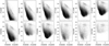 |
Fig. 1. Colour–magnitude diagrams. Each panel shows a different filter on the y-axis and F090W – F200W on the x-axis. Top row: HST filters from the HTTP. Bottom row: NIRCam filters. The RC sequence is visible as a straight sequence that is brighter and redder than the main sequence. |
3. Measuring extinction with red clump stars
Red clump (RC) stars are low-mass mass stars in their helium-burning phase that define a sharp feature in CMDs due their narrow range of intrinsic luminosity and colour (see the review Girardi 2016 or Onozato et al. 2019). They are excellent distance indicators (e.g., Grocholski & Sarajedini 2002), but also extinction affects their position in the CMD, making them to valuable tracers of interstellar extinction (e.g., Nataf et al. 2013; Sanders et al. 2022) as they scatter around the extinction vector. While the length of the so-formed RC sequence gives a handle on the maximum absolute extinction, its slope gives a direct measurement of the ratio R between absolute (A) and selective (E). This slope can be influenced by the line-of-sight depth (e.g., Yanchulova Merica-Jones et al. 2017), but this effect should be negligible in the LMC due to the its low inclination angle (∼25°) and small scale height (h ∼ 0.97 kpc; van der Marel & Cioni 2001; Ripepi et al. 2022). In the following, we describe our approach of selecting and then fitting the slope of RC stars in the CMDs (see Fig. 2).
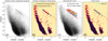 |
Fig. 2. Illustration of RC star selection. From left to right: panel a shows the original F090W – F200W CMD and panel b shows the same CMD after applying unsharp masking. We used this to obtain initial estimates for the blue and red end of the RC sequence as shown by the triangle symbols. Panel c shows the selection of RC stars using these initial estimates to obtain a selection region. Blue dots show all stars in this CMD falling into the selection region while orange dots show the final sample of stars that fall also in similar selection regions for other filter combinations. Panel d shows the final resulting fitted slope. |
3.1. Selecting RC stars
We inferred the nominal RC position (RC0) directly from the CMD as the blue, bright end of the elongated sequence. This is the position where unextinguished RC stars should be located. We used the unsharp masking technique to visually identify the RC, a similar approach to that described in De Marchi et al. (2016, 2021). Here, the CMD was first binned in a 2D array with a small binsize of 0.01 mag. Then, this histogram was convolved with a narrow, 2D Gaussian to assign each point a resolution that corresponds to the typical photometric uncertainty. We used 0.05 mag for the standard deviation of this Gaussian. In a second step, a broader Gaussian with a standard deviation of 0.2 mag was used to convolve this smoothed histogram even further and then the residual image was obtained by subtracting both blurred images from another. With this technique, features such as the RC become visible.
We used these images to get an initial estimate of the slope minit by identifying RC0 and a second, redder point (RC1), where the density of RC stars drops, however the RC sequence can extend to redder colours (see Fig. 2). To then select RC stars, we adopted the approach detailed in De Marchi & Panagia (2014): we selected all stars that are either in a error ellipse around the selected nominal RC position using conservative magnitude and colour uncertainties of 0.2 mag, respectively, or inside a region bounded by the tangents to this error ellipse with slopes minit ± 15%, extending past RC1. Allowing for a 15% uncertainty to the initial slope ensures that the selected sample is not biased with respect to the initial selection.
Using this selection yields an initial sample of RC stars for each filter (panel c in Fig. 2). To make the selection more robust against outliers, we considered only stars that were in the RC sample of at least ten of the twelve bands. At least 150 RC stars per filter are in this selection, with typical uncertainties of 0.02–0.04 mag.
3.2. Obtaining the extinction
We then fit the slope of the RC stars with a straight line using a least squares approach. To ensure the fits are stable against selection effects and photometric uncertainty, we fit each sample 10 000 times with a Monte Carlo approach. In each fit, the colour and magnitude of all RC stars are sampled randomly assuming Gaussian distributions for these parameters with standard deviations given by the photometric uncertainty. Additionally, we removed randomly 50% of the stars in each fit. We then defined the best-fitting slope as the mean of the resulting parameter distribution. As the uncertainty, we used the scatter of the residual.
Formally, the scatter around the best-fit value from the Monte Carlo approach might be used, which is typically around ∼0.02. However, as discussed in De Marchi et al. (2016), the dispersion around the best fit is a systematic effect due to varying grain sizes and a variable extinction law across the area. Additional scatter could be introduced by variations in the line-of-sight distance and stellar populations (Onozato et al. 2019).
4. Results
We fitted the RC slopes in CMDs using different filter combinations. These give the ratio R between absolute (A) and selective (E) extinction at different wavelengths λ:
We used both the F090W – F200W JWST and the F555W – F775W HST colours.
4.1. Extinction law
Figure 3 shows the extinction curve using the F090W – F200W and F555W – F775W colours. In the latter, we compare to the measurements presented in De Marchi et al. (2016) using the same HTTP HST data, but on a much larger area. As can be seen, our measurements fully reproduce the literature results, but now also include the much redder JWST filters and the narrow band filters F658N, F187N, and F470N. Table 1 reports the best-fitting extinction ratios for each filter. The extinction curves when using F090W – F200W or F555W – F775W colours are in full agreement.
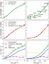 |
Fig. 3. Extinction law with linear (left) and logarithmic (right) x-axis. Top: green dots show the measured slopes of the RC stars using the F090W – F200W JWST colour. The solid line shows a univariate spline interpolation. Middle: red dots show the extinction curve as a function of F555W – F775W colours with results from De Marchi et al. (2016) (black dots) for optical wavelengths. Bottom: interpolated results for Aλ/E(V − I), compared to the MW extinction law (Fitzpatrick 1999) with RV = 3.1, corresponding to RV − I(V) = 2.3. Ratio and difference between those curves are shown by the orange dotted and purple dash-dotted lines, respectively. |
Measured ratios of absolute and selective extinction.
The solid lines in Fig. 3 show univariate spline interpolation of degree four through the measurements and shaded areas refer to interpolations through the measurements plus or minus uncertainties. Those interpolations were used to infer extinction values for other JWST NIRCam filters (see Table A.1).
The bottom panel of Fig. 3 shows the extinction law as Aλ/E(V − I) (see also De Marchi et al. 2016), compared with the MW curve from Fitzpatrick (1999). Based on extrapolations beyond the H band, De Marchi et al. (2016) suggested that at wavelength longer > 1 μm the extinction law in 30 Dor tapers off twice as quickly as the Galactic law because of the larger proportion of large grains in the 30 Dor interstellar medium adding a grey component to the extinction in the optical (and in the ultraviolet, De Marchi & Panagia 2019). With JWST, we can now confirm and extend this, finding the ratio to be relatively constant between 1 and 5 μm, suggesting the grain composition to be similar to that in the MW, but with a higher fraction of large grains. The ratio decreases for shorter wavelengths and reaches again constant values at λ ∼ 0.5 μm. For a discussion on grain sizes, we refer to De Marchi & Panagia (2019), who presented the extension of the 30 Dor extinction law into the ultraviolet.
4.2. Extinction map
Figure 4 shows the spatial distribution of RC stars on top of the F335M image, coloured by their absolute F090W extinction. The bottom panel presents an average extinction map and notes the average extinction and the standard deviation in each of the cells. For this figure, we redid the selection of RC stars using the derived slopes, a smaller uncertainty of 0.05 mag for the error ellipse, and no limitation at the red end.
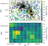 |
Fig. 4. Extinction map. Top: F335M mosaic of 30 Doradus (greyscale image) with individual RC stars (dots, colour-coded by their F090W extinction). Bottom: average F090W extinction in a grid of the same field-of-view. The mean extinction and the standard deviation are given by the number in each cell. The number of stars in each cell ranges from 5 to 28. |
The stars with highest extinction are located in and next to the web-like emission in the F335M image that follows the cold molecular gas (e.g., Wong et al. 2022). However, the cell with the lowest extinction in the field is located directly on top of a F335M-bright region. Due to low numbers and selection effects, we only used RC stars detected in F090W. In this highly embedded region, likely only foreground stars could be detected in this filter.
5. Discussion and conclusions
Figure 5 shows relative extinction curves expressed as Aλ/AV and Aλ/AKs using interpolated values for the V (0.551 μm) and 2MASS Ks (2.156 μm) bands. The top panel makes a comparison between the literature results from the MW (Fitzpatrick 1999; Wang & Chen 2019), and the LMC (Gordon et al. 2003; Wang & Chen 2023). The bottom panel makes a comparison with the central 3 × 3 deg2 of the MW from Sanders et al. (2022).
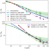 |
Fig. 5. Comparison of relative extinction with literature results. Top: extinction relative to AV assuming RF090W − F200W(AV) = 2.53 in green. Results for the MW in blue dashed (Fitzpatrick 1999) and purple (Wang & Chen 2019). Results for the LMC in cyan (Gordon et al. 2003) and orange (Wang & Chen 2023). Black show the UBVRIHJK values from De Marchi et al. (2016). Bottom: relative to AKs assuming RF090W − F200W(AV) = 0.45. Results from Sanders et al. (2022) for the MW in dark red, and from Fitzpatrick (1999) in blue. |
As also noted by Wang & Chen (2023), the extinction curve presented here and in De Marchi et al. (2016) is generally flatter than what is found for the average curves of much wider areas. This is likely caused by spatial variations in the grain size distribution and their relative abundances. As an exemplary massive and energetic star formation region, 30 Doradus is known to have an anomalous extinction law, as also discussed in De Marchi & Panagia (2014), Maíz Apellániz et al. (2014), De Marchi et al. (2016) or De Marchi & Panagia (2019). Here, we could show that this elevated extinction amplitude extends into the infrared and could confirm a transition in the slope at 1 μm.
For wavelengths > 1 μm, the slope in relative Aλ/AKs appears to follow the Galactic extinction law, implying a similar distribution of grain sizes. Our results might suggest a flattening of the curve at > 4 μm, but more measurements in the mid-infrared are needed to confirm this. The comparison of relative extinction curves reiterates what the comparison in Fig. 3 shows: the slope of the curve derived here matches the Galactic extinction laws at long wavelengths, but flattens out at shorter wavelengths. This highlights that while the nature of the grains is likely similar as in the MW, the size distribution differs, with 30 Doradus having a larger fraction of large grains.
To conclude, this Letter presents an extension of the extinction law in 30 Doradus to the infrared, exploiting the high resolving power of JWST. By combining the JWST NIRCam data with archival HST data, we derived a uniform extinction law from 0.3 to 4.7 μm using a fully consistent method based on the same field and the same stars. Compared with established extinction laws of the MW, we found both a higher value of RV − I and a change in the relative slope at ∼1 μm. At longer wavelengths, the ratio between curves is constant at ∼2, but decreases to ∼1.2 for wavelengths shorter than ∼0.5 μm, which is consistent with the presence of larger grains. In addition to the extinction law, we presented the spatial distribution of RC stars in the JWST NIRCam field-of-view and their absolute extinction in the F090W filter, finding that the most extinguished stars are in the highly embedded regions.
With its high star formation activity and low metallicity, 30 Doradus is often seen as a local analogue of high redshift star forming clumps. Consequently, the anomalous extinction law presented here has implications when interpreting results from high redshift, particularly as intrinsic fluxes might be underestimated when canonical6 MW laws are used.
Acknowledgments
We thank the anonymous referee for useful comments that helped polish this work. KF thanks Sam Pearson and Victor See for helpful discussions. KF acknowledges support through the ESA research fellowship programme. Based on observations with the NASA/ESA Hubble Space Telescope and the NASA/ESA/CSA James Webb Space Telescope, which are operated by AURA, Inc., under NASA contracts NAS5-26555 and NAS 5-03127. This work made use of Astropy: a community-developed core Python package and an ecosystem of tools and resources for astronomy (Astropy Collaboration 2013, 2018, 2022)
References
- Astropy Collaboration (Robitaille, T. P., et al.) 2013, A&A, 558, A33 [NASA ADS] [CrossRef] [EDP Sciences] [Google Scholar]
- Astropy Collaboration (Price-Whelan, A. M., et al.) 2018, AJ, 156, 123 [Google Scholar]
- Astropy Collaboration (Price-Whelan, A. M., et al.) 2022, ApJ, 935, 167 [NASA ADS] [CrossRef] [Google Scholar]
- Bressan, A., Marigo, P., Girardi, L., et al. 2012, MNRAS, 427, 127 [NASA ADS] [CrossRef] [Google Scholar]
- Castelli, F., & Kurucz, R. L. 2003, in Modelling of Stellar Atmospheres, eds. N. Piskunov, W. W. Weiss, & D. F. Gray, 210, A20 [Google Scholar]
- Castro, N., Crowther, P. A., Evans, C. J., et al. 2018, A&A, 614, A147 [NASA ADS] [CrossRef] [EDP Sciences] [Google Scholar]
- Crowther, P. A. 2019, Galaxies, 7, 88 [Google Scholar]
- Crowther, P. A., Broos, P. S., Townsley, L. K., et al. 2022, MNRAS, 515, 4130 [NASA ADS] [CrossRef] [Google Scholar]
- De Marchi, G., & Panagia, N. 2014, MNRAS, 445, 93 [NASA ADS] [CrossRef] [Google Scholar]
- De Marchi, G., & Panagia, N. 2019, ApJ, 878, 31 [NASA ADS] [CrossRef] [Google Scholar]
- De Marchi, G., Panagia, N., & Romaniello, M. 2010, ApJ, 715, 1 [NASA ADS] [CrossRef] [Google Scholar]
- De Marchi, G., Panagia, N., & Sabbi, E. 2011a, ApJ, 740, 10 [NASA ADS] [CrossRef] [Google Scholar]
- De Marchi, G., Paresce, F., Panagia, N., et al. 2011b, ApJ, 739, 27 [Google Scholar]
- De Marchi, G., Panagia, N., & Girardi, L. 2014, MNRAS, 438, 513 [NASA ADS] [CrossRef] [Google Scholar]
- De Marchi, G., Panagia, N., Sabbi, E., et al. 2016, MNRAS, 455, 4373 [CrossRef] [Google Scholar]
- De Marchi, G., Panagia, N., & Milone, A. P. 2021, ApJ, 922, 135 [NASA ADS] [CrossRef] [Google Scholar]
- Evans, C. J., Taylor, W. D., Hénault-Brunet, V., et al. 2011, A&A, 530, A108 [NASA ADS] [CrossRef] [EDP Sciences] [Google Scholar]
- Fitzpatrick, E. L. 1999, PASP, 111, 63 [Google Scholar]
- Girardi, L. 2016, ARA&A, 54, 95 [Google Scholar]
- Gordon, K. D., Clayton, G. C., Misselt, K. A., Landolt, A. U., & Wolff, M. J. 2003, ApJ, 594, 279 [NASA ADS] [CrossRef] [Google Scholar]
- Gouliermis, D. A., Henning, T., Brandner, W., et al. 2007, ApJ, 665, L27 [NASA ADS] [CrossRef] [Google Scholar]
- Grocholski, A. J., & Sarajedini, A. 2002, AJ, 123, 1603 [NASA ADS] [CrossRef] [Google Scholar]
- Indebetouw, R., Brogan, C., Chen, C. H. R., et al. 2013, ApJ, 774, 73 [NASA ADS] [CrossRef] [Google Scholar]
- Jones, O. C., Woods, P. M., Kemper, F., et al. 2017, MNRAS, 470, 3250 [NASA ADS] [CrossRef] [Google Scholar]
- Jones, O. C., Nally, C., Habel, N., et al. 2023, Nat. Astron., accepted [arXiv:2301.03932] [Google Scholar]
- Ksoll, V. F., Gouliermis, D. A., Klessen, R. S., et al. 2018, MNRAS, 479, 2389 [NASA ADS] [Google Scholar]
- Lopez, L. A., Grefenstette, B. W., Auchettl, K., Madsen, K. K., & Castro, D. 2020, ApJ, 893, 144 [NASA ADS] [CrossRef] [Google Scholar]
- Maíz Apellániz, J., Evans, C. J., Barbá, R. H., et al. 2014, A&A, 564, A63 [CrossRef] [EDP Sciences] [Google Scholar]
- Nataf, D. M., Gould, A., Fouqué, P., et al. 2013, ApJ, 769, 88 [Google Scholar]
- Nayak, O., Green, A., Hirschauer, A. S., et al. 2023, ApJ, 944, 26 [NASA ADS] [CrossRef] [Google Scholar]
- Onozato, H., Ita, Y., Nakada, Y., & Nishiyama, S. 2019, MNRAS, 486, 5600 [NASA ADS] [CrossRef] [Google Scholar]
- Panagia, N. 2005, IAU Colloq. 192: Cosmic Explosions, On the 10th Anniversary of SN1993J, eds. J.-M. Marcaide, & K. W. Weiler, 99, 585 [NASA ADS] [CrossRef] [Google Scholar]
- Panagia, N., Gilmozzi, R., Macchetto, F., Adorf, H. M., & Kirshner, R. P. 1991, ApJ, 380, L23 [NASA ADS] [CrossRef] [Google Scholar]
- Reiter, M., Morse, J. A., Smith, N., et al. 2022, MNRAS, 517, 5382 [NASA ADS] [CrossRef] [Google Scholar]
- Ripepi, V., Chemin, L., Molinaro, R., et al. 2022, MNRAS, 512, 563 [NASA ADS] [CrossRef] [Google Scholar]
- Sabbi, E., Anderson, J., Lennon, D. J., et al. 2013, AJ, 146, 53 [NASA ADS] [CrossRef] [Google Scholar]
- Sabbi, E., Lennon, D. J., Anderson, J., et al. 2016, ApJS, 222, 11 [NASA ADS] [CrossRef] [Google Scholar]
- Sanders, J. L., Smith, L., González-Fernández, C., Lucas, P., & Minniti, D. 2022, MNRAS, 514, 2407 [CrossRef] [Google Scholar]
- Sun, N.-C., de Grijs, R., Subramanian, S., et al. 2017, ApJ, 835, 171 [NASA ADS] [CrossRef] [Google Scholar]
- van der Marel, R. P., & Cioni, M.-R. L. 2001, AJ, 122, 1807 [Google Scholar]
- Wang, S., & Chen, X. 2019, ApJ, 877, 116 [Google Scholar]
- Wang, S., & Chen, X. 2023, ApJ, accepted [arXiv:2301.09146] [Google Scholar]
- Wong, T., Oudshoorn, L., Sofovich, E., et al. 2022, ApJ, 932, 47 [NASA ADS] [CrossRef] [Google Scholar]
- Yamane, Y., Sano, H., Filipović, M. D., et al. 2021, ApJ, 918, 36 [NASA ADS] [CrossRef] [Google Scholar]
- Yanchulova Merica-Jones, P., Sandstrom, K. M., Johnson, L. C., et al. 2017, ApJ, 847, 102 [NASA ADS] [CrossRef] [Google Scholar]
Appendix A: Interpolated values for other JWST NIRCam filters
Table A.1 reports the ratio of absolute and selective extinction for other NIRCam filters. These values are based on the univariate spline interpolation (see Sect. 4). The uncertainties are based on the envelope curves using interpolation of the measured values plus or minus the measured dispersion around the residual. For interpolated values in common optical filters, we refer to De Marchi et al. (2016).
Interpolated extinction values for different JWST NIRCam filters.
All Tables
All Figures
|
Fig. 1. Colour–magnitude diagrams. Each panel shows a different filter on the y-axis and F090W – F200W on the x-axis. Top row: HST filters from the HTTP. Bottom row: NIRCam filters. The RC sequence is visible as a straight sequence that is brighter and redder than the main sequence. |
| In the text | |
|
Fig. 2. Illustration of RC star selection. From left to right: panel a shows the original F090W – F200W CMD and panel b shows the same CMD after applying unsharp masking. We used this to obtain initial estimates for the blue and red end of the RC sequence as shown by the triangle symbols. Panel c shows the selection of RC stars using these initial estimates to obtain a selection region. Blue dots show all stars in this CMD falling into the selection region while orange dots show the final sample of stars that fall also in similar selection regions for other filter combinations. Panel d shows the final resulting fitted slope. |
| In the text | |
|
Fig. 3. Extinction law with linear (left) and logarithmic (right) x-axis. Top: green dots show the measured slopes of the RC stars using the F090W – F200W JWST colour. The solid line shows a univariate spline interpolation. Middle: red dots show the extinction curve as a function of F555W – F775W colours with results from De Marchi et al. (2016) (black dots) for optical wavelengths. Bottom: interpolated results for Aλ/E(V − I), compared to the MW extinction law (Fitzpatrick 1999) with RV = 3.1, corresponding to RV − I(V) = 2.3. Ratio and difference between those curves are shown by the orange dotted and purple dash-dotted lines, respectively. |
| In the text | |
|
Fig. 4. Extinction map. Top: F335M mosaic of 30 Doradus (greyscale image) with individual RC stars (dots, colour-coded by their F090W extinction). Bottom: average F090W extinction in a grid of the same field-of-view. The mean extinction and the standard deviation are given by the number in each cell. The number of stars in each cell ranges from 5 to 28. |
| In the text | |
|
Fig. 5. Comparison of relative extinction with literature results. Top: extinction relative to AV assuming RF090W − F200W(AV) = 2.53 in green. Results for the MW in blue dashed (Fitzpatrick 1999) and purple (Wang & Chen 2019). Results for the LMC in cyan (Gordon et al. 2003) and orange (Wang & Chen 2023). Black show the UBVRIHJK values from De Marchi et al. (2016). Bottom: relative to AKs assuming RF090W − F200W(AV) = 0.45. Results from Sanders et al. (2022) for the MW in dark red, and from Fitzpatrick (1999) in blue. |
| In the text | |
Current usage metrics show cumulative count of Article Views (full-text article views including HTML views, PDF and ePub downloads, according to the available data) and Abstracts Views on Vision4Press platform.
Data correspond to usage on the plateform after 2015. The current usage metrics is available 48-96 hours after online publication and is updated daily on week days.
Initial download of the metrics may take a while.