| Issue |
A&A
Volume 676, August 2023
|
|
|---|---|---|
| Article Number | A141 | |
| Number of page(s) | 12 | |
| Section | The Sun and the Heliosphere | |
| DOI | https://doi.org/10.1051/0004-6361/202346183 | |
| Published online | 22 August 2023 | |
Modeling the formation and eruption of coronal structures by linking data-driven magnetofrictional and MHD simulations for AR 12673⋆
1
Department of Physics, University of Helsinki, Helsinki, Finland
e-mail: This email address is being protected from spambots. You need JavaScript enabled to view it.
2
NASA Goddard Space Flight Center, Greenbelt, MD 20771, USA
Received:
19
February
2023
Accepted:
4
July
2023
Abstract
Context. The data-driven and time-dependent modeling of coronal magnetic fields is crucial for understanding solar eruptions. These efforts are complicated by the challenges of finding a balance between physical realism and computing efficiency. One possible technique is to couple two modeling approaches.
Aims. Our aim here is to showcase our progress in using time-dependent magnetofrictional model (TMFM) results as input to dynamical magnetohydrodynamic (MHD) simulations. However, due to the different evolution processes in these two models, using TMFM snapshots in an MHD simulation is nontrivial. We address these issues, both physically and numerically, discuss the incompatibility of the TMFM output to serve as the initial condition in MHD simulations, and show our methods of mitigating this. The evolution of the flux systems and the cause of the eruption are investigated.
Methods. TMFM is a prevalent approach that has proven to be a very useful tool in the study of the formation of unstable structures in the solar corona. In particular, it is capable of incorporating observational data as initial and boundary conditions and requires shorter computational time compared to MHD simulations. To leverage the efficiency of data-driven TMFM and also to simulate eruptive events in the MHD framework, one can apply TMFM up to a certain time before the expected eruption(s) and then proceed with the simulation in the full or ideal MHD regime in order to more accurately capture the eruption process.
Results. We show the results of a benchmark test case with a linked TMFM and MHD simulation to study the evolution of NOAA active region 12673. A rise of a twisted flux bundle through the MHD simulation domain is observed, but we find that the rate of the rise and the altitude reached depends on the time of the TMFM snapshot that was used to initialize the MHD simulation and the helicity injected into the system. The analysis suggested that torus instability and slip-running reconnection could play an important role in the eruption.
Conclusions. The results show that the linkage of TMFM and zero-β MHD models can be successfully used to model the eruptive coronal magnetic fields.
Key words: Sun: corona / magnetohydrodynamics (MHD) / methods: numerical
Movie associated to Fig. 6 is available at https://www.aanda.org.
© The Authors 2023
 Open Access article, published by EDP Sciences, under the terms of the Creative Commons Attribution License (https://creativecommons.org/licenses/by/4.0), which permits unrestricted use, distribution, and reproduction in any medium, provided the original work is properly cited.
This article is published in open access under the Subscribe to Open model. This email address is being protected from spambots. You need JavaScript enabled to view it. to support open access publication.
1. Introduction
Modeling eruptive coronal magnetic fields is a key element for obtaining knowledge of the dynamics and underlying physical mechanisms of coronal mass ejections (CMEs; e.g., Welsch 2018). CMEs erupt regularly from the Sun, and they consist of huge helical flux ropes (Chen 2017) where magnetic field lines wind about a common axis. They can cause drastic disturbances in heliospheric plasma and field conditions, and therefore are primary drivers of space weather at Earth and other planets of our Solar System (e.g., Webb & Howard 2012; Kilpua et al. 2017).
This paper studies the active region (AR) 12673 which was visible on the solar disk from late August 2017 through September 10, 2017. This AR produced a number of big flares and CMEs and has been a subject of several studies (e.g., Yang et al. 2017; Chertok et al. 2018; Hou et al. 2018; Inoue et al. 2018b; Jiang et al. 2018; Liu et al. 2018; Verma 2018; Yan et al. 2018; Morosan et al. 2019; Price et al. 2019; Romano et al. 2019; Zou et al. 2019, 2020; Inoue & Bamba 2021). We focus here on the eruption on September 6, 2017, which featured an X9.3 flare at 11:53 UT and a fast CME, which was first detected in the STEREO/COR2 coronagraph field of view around 12:24 UT. Several studies have shown that this eruption involved a multiflux-rope system above the polarity inversion line located in the middle of the AR (e.g., Hou et al. 2018; Inoue et al. 2018b; Price et al. 2019). The flux rope formed prior to the eruption due to the shearing motions related to the sunspot rotation (Yang et al. 2017; Yan et al. 2018; Zou et al. 2019). Both the kink instability (Hou et al. 2018) and torus instability (Zou et al. 2019; Inoue & Bamba 2021) have been invoked as the eruption mechanism for this event.
Several of the above cited studies have used magnetohydrodynamic (MHD) simulations of the corona initiated by nonlinear force-free-field (NLFFF) modeling (Jiang et al. 2018; Inoue et al. 2018b; Inoue & Bamba 2021). The study by Jiang et al. (2018) reproduced some features of the eruptive X9.3 flare in great detail, including multiple twisted flux systems that finally reconnected via tether cutting to form one coherent flux rope. Similarly, Inoue et al. (2018b) found a coherent and highly twisted flux rope forming from reconnection between smaller flux ropes that were located along the magnetic polarity inversion line. They also reported a writhing of the flux rope which refers to the helical deformation of the flux rope axis. The further study by Inoue & Bamba (2021) modeled both an earlier strong flare (X2.2) on September 6 at 08:57 UT and the X9.3 flare. The authors used NLFFF to reconstruct the magnetic field approximately two hours before the X2.2 flare and they used this as the initial condition of the MHD model. The simulation showed that the flux rope that formed beneath the field lines was repelled upward by the first flare via continuous reconnection. This reconnection built up the magnetic flux in the flux rope, which was lifted up and eventually erupted via the torus instability.
Price et al. (2019) performed a data-driven and time-dependent magnetofrictional (TMFM; Pomoell et al. 2019) simulation of the event. The obtained modeling results were compared to the flux rope observations in AIA 94 Å images during the eruptive event. This study also suggested a value for the ratio of current-carrying helicity to relative helicity as the criteria of an eruptive event, which was in agreement with Pariat et al. (2017) and Zuccarello et al. (2018). The TMFM approach also captured the key eruption dynamics and found that the flux rope formed from a combination of two twisted flux systems which partially combined during the eruption process.
An advantage of the TMFM model is that it is computationally efficient and requires only boundary conditions derived from (vector) magnetograms as its input. However, due to the simplified momentum equation, it is not able to capture the dynamic evolution of eruptive events accurately with the rate of evolution being much slower than observed events (Pomoell et al. 2019; Jiang et al. 2021).
To overcome the lack of dynamic evolution in an extrapolated magnetic field using an NLFFF approach, and to capture more accurately the evolution of the system under study using a more realistic momentum equation, in this paper we use the data-driven TMFM model employed by Price et al. (2019) to study the eruption related to the X9.3 flare on September 6, 2017 from NOAA AR 12673 to initiate the magnetic field in an ideal MHD simulation. We assume that the evolution of the system is dominated by the magnetic field, that is we employ the zero-β approximation. The mass density of the plasma is estimated with an initially constant Alfvén velocity in the entire computational box. This change in the modeling framework is not trivial due to different equations governing the evolution of the system of interest. Using the output of efficient time-dependent coronal models in dynamically more accurate magnetohydrodynamic simulations has been considered previously. For instance, Pagano et al. (2013) used the output of a magnetofrictional model of the long-term evolution of two idealized magnetic bipoles, in which a flux rope is formed along the polarity inversion line, as the initial condition for an MHD simulation to study the eruption of the flux rope. More recently, Inoue et al. (2023) considered the effect of different boundary prescriptions when linking time-dependent MHD models.
The paper is organized as follows: A short overview of the models employed to prepare the initial conditions (data-driven time-dependent magnetofrictional) and the ideal zero-β MHD driving the simulation are presented in Sect. 2. In Sect. 3 we briefly described the numerical setup of MHD simulation code, followed by Sect. 4 in which the effects of the different initial conditions on the system’s evolution and the possible instability driving the eruption are discussed. At the end, we dedicate Sect. 5 to our conclusions of the approach presented in this work.
2. Models
2.1. Zero-β ideal MHD modeling
To advance beyond the assumption of quasi-static dynamical evolution employed by the magnetofrictional method, we consider a magnetohydrodynamic description of the dynamics in the active region. As the magnetic field dominates the evolution of the system compared with gravity and thermal pressure in the vicinity of the strong magnetic fields in the active region, we simplified the dynamical model by neglecting the thermal pressure thereby assuming the plasma β to be zero throughout the domain. Due to the applicability of this description to active region environments in the low corona, the zero-β MHD model is often employed to simulate coronal dynamics in such environments as in Kliem et al. (2004), Török et al. (2004, 2013), Inoue et al. (2014, 2018a, 2023), Inoue (2016), and Guo et al. (2019). The zero-β MHD description of the plasma that we employed is given by the following set of conservation laws:
 (1)
(1)
 (2)
(2)
 (3)
(3)
 (4)
(4)
in which ρ, V, B, E are the mass density, plasma bulk velocity, magnetic field, and electric field, respectively. It is important to note that the mass density is evolved according to the continuity equation. In some zero-β models, the continuity equation is replaced by a quasi-evolution of the mass density by imposing directly a functional form, typically a function of the magnetic field magnitude, that explicitly determines the mass density at each time (e.g., Inoue & Bamba 2021).
2.2. Data-driven time-dependent magnetofrictional model
The zero-β MHD model, described in the previous subsection, is initiated with the magnetic field provided by a data-driven time-dependent magnetofrictional model (TMFM). The detailed description of this model is given in Pomoell et al. (2019), while the application of the model to the event under consideration is described in Price et al. (2019). In the following, we provide a brief overview of the model.
In the TMFM model, the response of the coronal magnetic field to the comparatively slow photospheric changes is assumed to proceed largely as a quasi-static evolution from an equilibrium state to the next (Ballegooijen et al. 2000; Chitta et al. 2014).
Similar to the zero-β MHD model, gravity, thermal pressure, and other thermodynamic processes are ignored.
With these assumptions the momentum equation reduces to an explicit relation for the plasma velocity that is proportional to the Lorentz force. The specific form is given by
 (5)
(5)
where ν is the magnetofrictional coefficient. The magnetofrictional model thus amounts to solving Faraday’s law employing a resistive Ohm’s law with the velocity field provided by Eq. (5). With this prescription, the system relaxes toward a force-free state in the absence of a net Poynting flux subjected on the system. If time-dependent boundary conditions are used, a force-free state is in general not reached and the coronal magnetic field evolves dynamically. The speed at which the magnetic field in the model responds to departures from force-free equilibria scales by the inverse of the magnitude of the magnetofrictional coefficient, and is constrained by considering the time scales of the photospheric driving and assumption of quasi-static coronal evolution (see Pomoell et al. 2019; Cheung & DeRosa 2012, for a further discussion).
To drive the evolution of the coronal magnetic field, the photospheric electric field is required as input to the magnetofrictional model. The evolution of the photospheric magnetic field, obtained from a time-sequence of vector magnetograms, is sufficient to determine the inductive component of the electric field. However, recent studies have highlighted that to describe dynamics of the coronal magnetic fields it is critical to include the noninductive electric field component (e.g., Cheung & DeRosa 2012; Pomoell et al. 2019) which can be understood from the perspective of the transport of magnetic helicity and free energy from the photosphere to the corona (Schuck & Antiochos 2019). In Lumme et al. (2017), an optimization-based approach to constrain the noninductive component was presented. In this method, a functional form describing the (horizontal) divergence of the noninductive photospheric electric field is assumed. The free parameter included in the functional form is then determined such that the energy injection is matched with a given reference estimate.
In Price et al. (2019), the energy injection was optimized using the DAVE4VM result as reference. For further information on the inversion procedure as well as the magnetofrictional evolution for the particular time under consideration, the reader is referred to Price et al. (2019). For the current study, in addition, a second TMFM simulation run was carried out with an increased value for the free parameter controlling the magnitude of the noninductive component. Finally, we note that while the vector magnetogram data was used in the electric field inversion, the sole boundary condition to the time-dependent magnetofrictional model are the two components of the horizontal photospheric electric field. As a result, the horizontal components of the magnetic field closest to the photospheric boundary evolve self-consistently via the imposed photospheric electric field and the TMFM electric field and are not fixed to match the horizontal photospheric magnetic field data.
2.3. Employing TMFM as initial condition to MHD
In contrast to the TMFM model, the zero-β MHD model considered in this work requires not only the magnetic field to be given as an initial condition, but also the mass density and plasma flow velocity need to be specified at t = 0.
Here, we set the initial mass density by assuming that the Alfvén speed is initially constant in the simulation domain, specifically:
 (6)
(6)
where vA is a given constant, and the initial magnetic field B(r, t = 0) in the MHD simulation is identical to the magnetic field given by the TMFM model at a specified time.
In addition, we set the initial flow speed equal to zero, that is V(r, t = 0) = 0, everywhere in the domain. The choice of initially setting the flow speed to zero and choosing the mass density according to Eq. (6) is motivated as follows. With this choice, the time-derivatives of the mass density and magnetic field are initially zero, while for the plasma velocity we have initially
 (7)
(7)
where VMFM is the velocity field of the TMFM model associated with the given magnetic field configuration which is defined by Eq. (5). Thus, with this setup, the initial dynamics in the zero-β MHD model is directly proportional to the magnetofrictional velocity, or equivalently, proportional to the Lorentz force. Here, we should emphasize that the velocity field in the TMFM and MHD model descriptions have significantly different interpretations. In TMFM the VMFM is chosen specifically so that plasma evolves toward a force-free state, whereas in the MHD description the plasma has inertia. Thus, we do not use VMFM for specifying the initial MHD flow velocity. Unless otherwise noted, in this work we set vA = 300 km s−1 for all simulation runs. We repeated several simulation runs using different values for vA. For all cases, we observed changes in the dynamics largely consistent with the scale invariance of the ideal MHD system of equations. Thus, the time scales of the dynamics presented in this work is to a degree arbitrary. Nevertheless, we choose to present the results using dimensional units of time as given by the specific choice of vA.
2.4. MHD boundary conditions and numerical aspects
As mentioned previously, the basic premise of the modeling in this work is to employ the time-dependent magnetofrictional method to model the quasi-static evolution of the active region magnetic field prior to and through the emerging phase up to a given time at which the magnetic field is transferred to and subsequently evolved using a zero-β MHD simulation. In contrast to the data-driven TMFM model, after the point of transfer, the MHD system is no longer driven at the photospheric boundary, and instead a line-tied boundary condition is implemented. Thus, on the lower boundary the normal component of the magnetic field remains fixed in time, which is accomplished by setting the horizontal electric field equal to zero, and the normal component of the magnetic field is identical to the normal component of the TMFM snapshot used to initialize the MHD computation. In addition, the mass density at the lower boundary is kept fixed, and the velocity set to zero. At the top and lateral boundaries, an open boundary condition is mimicked by imposing zero-gradient extrapolation in the direction of the surface normal.
We note that a similar choice of boundary conditions was recently successfully employed by Inoue et al. (2023) when using the output from a data-driven MHD model as the initial condition in a simulation that was not driven.
The MHD equations are solved using a second-order accurate method that uses a cell-centered finite-volume scheme for the hydrodynamic variables while the electromagnetic fields are treated using a staggered constrained transport (CT) scheme similar to our previous work (Pomoell et al. 2008; Hoilijoki et al. 2013). It is important to note that the CT scheme keeps the divergence of the magnetic field unchanged throughout the evolution up to the accuracy of the floating-point arithmetic operations. Thus, the divergence of the magnetic field is required to be identically zero for the initial condition, which is guaranteed by the numerical approach used in the TMFM model (see Pomoell et al. 2019 for details). As in the TMFM model, the computational domain spans a size of 360 × 280 × 200 Mm with the same grid resolution used in both models. As a result, the magnetic field can be simply directly copied from the TMFM model to the MHD computational grid without any intermediate processing steps.
3. Choice of TMFM snapshot transfer times
The choice of the time at which the magnetic field configuration of the TMFM solution is transferred to initialize the MHD computation is not constrained a priori. In this work we used TMFM simulation with the optimized Ω (Ωopt) and with 1.5 times the optimized Ω. The latter describes a case where additional energy and helicity as compared to DAVE4VM is injected into the system. The initial condition from the two TMFM simulations was selected for the MHD simulation at three different times, resulting in distinct dynamical behaviors as discussed in the following sections.
In the following, we define the reference time (denoted tref) to be on September 6, 2017 at 09:24:00 UT that corresponds approximately to the time of the observed eruptive X-class flare (the flare occurred at 11:53 UT). At this time, the flux rope had started its rise in the TMFM simulation as analyzed in Price et al. (2019) in which the optimized value for Ω was used in the electric field inversion. We remind that the merging of two twisted flux systems to one larger flux rope as reported in previous studies (see the Introduction) occurred before the reference time.
Two other snapshots from the TMFM simulation were also selected as initial condition for separate MHD runs, chosen here to be 24 (denoted t−24) and 12 h (denoted t−12) before the reference time. The goal for selecting multiple snapshots is to analyze the potential sensitivity of the resulting dynamics on the initial condition. In particular, as the reference time corresponds to the time closest to the time of the actual observed eruption from the selected snapshots, the aim is to test whether this is reflected in the dynamics of the model. In addition, since the two models differ in the physical description of the evolution of the magnetic field, it is important to verify that any possible eruption is due to the state of the system under study and not solely a result of changing the simulation framework.
4. Analysis and results
4.1. Overall dynamics of the magnetic field configuration
In Fig. 1, the overall dynamics of the magnetic field of the active region in the zero-β simulation is shown when initialized at two separate instances of time, at time t−24, which is 24 h prior to the reference time (left panels) and at the reference time (right panels). The results from the two separate TMFM runs using different noninductive photospheric electric field data are also shown featuring different amount of energy and helicity injected into the system (Ωopt and 1.5 × Ωopt; Sect. 3).
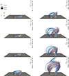 |
Fig. 1. Snapshots of the zero-β MHD simulation showing the evolution of the multiflux system preceding the September 6, 2017 flare and its accompanying CME eruption. The top and third rows show the initial situation for the simulations (t = 0) and the second and bottom rows the simulations at time t = 600 s. The left panels give results when the zero-β MHD simulation was initialized with the TMFM snapshot at time t−24, i.e., 24 h before the reference time, while the right panels show the results when the initialization was made at the reference time (September 6, 2017 at 09:24 UT). The two top panels give the results when the TMFM simulation was performed with the optimized Ω and the bottom rows when it was performed with 1.5 times the optimized Ω. The color of the field lines were selected in order to facilitate the visual distinguishability of the flux systems. |
The figure features three sets of field lines with each set using a distinct color map for coloring the field lines based on their magnetic connectivity. We first note that for the t−24 initialization and Ωopt case a large-scale twisted flux rope did not form during the simulation time and the flux systems involved did not rise significantly. For the reference time runs and the t−24 flux rope in the 1.5 × Ωopt case the blue-white field lines feature the flux rope that had merged from the initial two twisted flux ropes as discussed in Sect. 1, while the yellow-purple field lines show the twisted arcade-like structure overlying the flux rope. The white-purple field lines show the arcades close to the bottom part of the simulation domain that form the null-point with the flux systems above and reconnect with them during the eruption. The gray-scale color map at the bottom shows the vertical magnetic field component at the bottom of the simulation domain that corresponds to the photospheric (magnetogram) plane.
The times in the snapshots were selected to demonstrate the differences in the ascent rates of the flux ropes in those MHD simulations where the flux rope formed (i.e., all others except the t−24 initialization with Ωopt). The panels in the top and third rows show the situation at the start of the zero-β MHD simulations when the magnetic field is identical to that of the input TMFM field. The panels on the second and the bottom row show the magnetic field configuration in the zero-β MHD simulation after 600 s of evolution.
At the beginning of the zero-β MHD simulation (t = 0), the flux system containing twisted magnetic fields (blue-white and yellow-purple systems) is located higher when the TMFM configuration at the reference time is used as the initial condition than when the snapshot was taken 24 h earlier. This change reflects the evolution of the flux system in the TMFM simulation wherein a large-scale flux rope is clearly identifiable in the simulation (see e.g., Fig. 9 in Price et al. 2019). In addition, for the reference time simulations the flux rope is clearly at a higher altitude at t = 0 for the case where the TMFM was run with 1.5 × Ωopt compared to the Ωopt case. This is a direct consequence of the more dynamic evolution in TMFM as a response to the increased injection of energy and helicity by the photospheric electric field. As discussed above, for the t−24 initialization with Ωopt we did not find a large-scale rising twisted flux rope. This is featured by comparing the two top left panels, that is, the flux systems in the vicinity of the AR remain largely unchanged after 600 s of evolution. In contrast, for the 1.5 × Ωopt case, a flux rope is identifiable and is seen to rise in the t−24 run. For the Ωopt case the reference time flux systems stay within the simulation box, while for the 1.5 × Ωopt case the field lines of the blue-white system have started to exit the simulation box at t = 600 s.
To quantify the behavior of the flux systems in the vicinity of the core of the active region, which is around the main polarity inversion line (PIL) hosting the flux rope, we compute the change over time of the lengths and maximum heights of field lines. Specifically, for each simulation cell at the photospheric (z = 0) height, a field line is traced and its maximum height h and length l is recorded. From this data, the change in the maximum height Δh = h(t)−h(t = 0) compared to the initial height of each field line is determined. This allows visualization of the changes in the flux system that are rooted in the photosphere during the evolution in the MHD simulations. It is important to note that this analysis is robust due to the line-tying boundary condition in the zero-β simulation in contrast to the TMFM simulation.
In Fig. 2, the change in field line heights from their initial heights to that at t = 600 s is shown. During this period in this region, most of the field lines rooted in the photosphere undergo only small changes in their heights. Thus, field lines for which the change in height is less than 5 Mm are masked. The significant changes in the field line heights are observed to take place away from the main PIL for all three cases. Furthermore, most of the larger changes (|Δh|≳60 Mm) occur for field lines that are already long at the start of the simulation run. This is indicated by the two over-plotted contour lines which show regions of field lines that are 100 Mm (orange solid contour) and 200 Mm (black dashed contour) in total length at t = 0. As is seen, the largest changes (dark red and dark blue) fall within the 200 Mm contour. These results show that most of the evolution, in particular for the −24 h (shown in panel a) and −12 h cases (shown in panel b) takes place for the large field lines overlying the AR that continue to mostly rise. In contrast, field lines that initially are relatively short undergo notable changes only in small isolated regions.
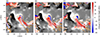 |
Fig. 2. Change of the maximum height of field lines rooted in the photosphere at time t = 600 s compared to their initial height, Δh = h(t = 600)−h(t = 0). Panels from left to right show the result for the simulations initialized at t−24, t−12 and the reference time, respectively, using Ωopt. The orange solid (black dashed) contour indicates field lines of lengths 100 (200) Mm. The gray scale shows the vertical component of photospheric magnetic field saturated at ±0.1 T. |
4.2. Dynamical evolution of key flux systems
To quantitatively compare the dynamical evolution of the system across the different simulation runs, we compute changes in field line heights as a function of time as well as investigate the energy evolution. Figure 3 shows the results of these computations for the MHD simulations initialized at the reference time (black curves) as well as for the simulations initialized at t−24 (reference time – 24 h, purple curves) and t−12 (reference time – 12 h, green curves). In all panels, the solid curves show the results for the Ωopt TMFM input and the dashed curves for the 1.5 × Ωopt simulations.
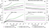 |
Fig. 3. Parametric evolution of the zero-β MHD simulation. The panels show: a) the apex altitude of the main flux rope, b) the ratio of the free to total magnetic energy, c) kinetic energy, and d) the slab magnetic energy as a function of simulation time (in seconds) in the zero-β MHD simulation. The black curve shows the run where the MHD simulation was initialized with the TMFM snapshot at the reference time, and the purple (green) curves the case where the simulations were initialized 24 (12) h before the reference time. The solid curves show the results for the optimized Ω and the dashed lines for the 1.5 × optimized Ω. The tracking is continued until the boundary effects start to take over when the flux rope approaches the top of the simulation box (case for the reference time run with 1.5 × Ωopt), see the text for details. |
In Fig. 3a, the evolution in time of the maximum height of a bundle of field lines rooted in the photosphere is shown. The selected photospheric foot-points, kept fixed in time, of the bundles are indicated in Fig. 2 by the blue circles. These specific locations were determined so as to be representative of the dynamics of the flux system that includes the flux rope that forms and rises in the simulations. As the bundles contain several field lines with different maximum heights that are tracked, the result from the individual field lines of the bundle are then averaged and finally shown in panel a. The difference in height at the start of the three initialization times reflects the fact that the magnetic field continues to evolve in the TMFM simulation, with the tracked flux system located initially highest at the reference time (see also Sect. 4.1).
For the Ωopt run (solid curves) the reference time and t−12 tracked flux bundle rises consistently through the simulation time reaching altitudes of ∼110 and ∼75 Mm, respectively. We note that the differences in the final heights reached are largely due to different starting heights in the simulation. The flux bundle for the t−24 run shows nearly no change in height.
For the simulations initiated using the 1.5 × Ωopt results, the flux bundles rise distinctly faster, however, only after an initial phase in which the change in height is comparable to the corresponding simulation initialized using Ωopt. The reference time and t−12 flux bundles rise considerably faster than the t−24 flux bundles. However, for the t−12 case, the rise flattens toward the end of the simulation when the altitude of ∼140 Mm was reached. In contrast, the height of the reference time flux bundle using the 1.5 × Ωopt result increases rapidly and reaches the top boundary of the simulation box at approximately t = 450 s. At this point the tracking of the bundle was stopped. This is also visible in the bottom right panel of Fig. 1 that shows a number of the field lines exiting the simulation box at t = 600 s. For the t−24 case the flux bundles rise consistently and reach almost the same height (∼125 Mm) as the t−12 flux bundles by the end of the simulation.
The top right panel of Fig. 3 shows the ratio EF/EM of the free EF to total magnetic energy EM. The total magnetic energy is calculated as
 (8)
(8)
and the free energy is here defined as EF = EM − EP where EP is the magnetic energy of the corresponding potential magnetic field.
For both the Ωopt and the 1.5 × Ωopt cases the free to total magnetic energy ratio is the largest for the reference run and smallest for the run initialized 24 h before the reference run. This is an expected trend because, as shown in Fig. 4 of Price et al. (2019), the ratio tended to increase until the time of the flare. The reference time had the most time to evolve, and therefore could accumulate more energy via flux emergence before the TMFM snapshot was used to initialize the zero-β MHD simulation.
For all cases the ratio decreases monotonically throughout the simulation. This is because the zero-β MHD simulation is essentially a relaxation simulation as no new energy is injected into the system. As expected, the free to total magnetic energy ratio is larger for the 1.5 × Ωopt case than for Ωopt because more energy and helicity is injected into the system in the TMFM simulation.
Panel c in Fig. 3 gives the total kinetic energy in the simulation volume as a function of time. For the reference time and t−12 for the 1.5 × Ωopt case the kinetic energy increases significantly with clearly the largest values for the reference time. For other cases the increase is clearly more modest and the curves flatten after an initial increase. The increase can be partly attributed to free magnetic energy transferring into kinetic energy. We note that as the kinetic energy is computed for the entire simulation volume, the changes are not directly attributable to the dynamics of the flux rope and associated flux system, as also other dynamics take place in the simulation domain.
The right bottom panel shows the total magnetic energy computed for a given portion V1 of the simulation domain. The sub volume V1 is defined as the volume V1 = [ − 90, 40]×[−64, 86]×[40, 60] (all in Mm) and is chosen to cover the main AR horizontally and an intermediate height range. For all simulation runs, a similar overall trend is visible: a steady initial phase followed by an increase, after which a steady decrease or saturation is observed. The simultaneous on-set of the increase across the simulation runs is a reflection of the same constant Alfvén speed chosen when initializing the MHD simulation. The consistent overall trend shows that for all runs, magnetic energy enters the upper heights of the simulation, and a significant fraction of the energy continues to rise and exits the subdomain. For all cases except the reference time run initialized using the 1.5 × Ωopt result, the energy in the subdomain is larger at the end than at the start. Only for the one run the net change of magnetic energy is negative in this subdomain, reflecting the expulsion of the flux systems that is observed to take place in the simulation.
4.3. Evolution of the force-freeness of the magnetic field
Since the dynamics of the zero-β simulation is driven by the Lorentz force, we next investigate how force-free the magnetic field is and how it varies in time. The results are gathered in Fig. 4 that shows the current-weighted sine (CWsin) force-freeness metric both in the TMFM simulation (left panels) and in the zero-β MHD simulation (right panels). CWsin is a metric that quantifies how force-free the magnetic field is over the given volume, and is often used to evaluate the success of force-free magnetic field extrapolations. It is calculated as the current-weighted sine between the current density and the magnetic field (Metcalf et al. 2008):
 (9)
(9)
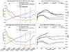 |
Fig. 4. Comparison of force-freeness and free magnetic energy in the TMFM and zero-β MHD simulations. Left panels: evolution of CWsin force-freeness factor during TMFM simulation of the entire computational box (blue) and a box enclosing the main flux rope (orange). The black curves show the evolution of free magnetic energy for the whole domain (solid curve) and the subdomain (dashed curve). The reference time (black), and times 12 (green) and 24 (purple) h before the reference time are shown by dashed vertical lines. Right panels: time evolution of CWsin in the zero-β MHD simulation for the whole domain (solid) and subdomain (dashed). The top panels show the results for the optimized Ω and the bottom panels for the 1.5 × optimized Ω. |
where the summation runs over grid locations ı and where σı is the absolute value of the sine of the angle between the current density and magnetic field at the given grid location:
 (10)
(10)
This parameter is zero for a strictly force-free-field and increases towards 1 as the angle between the current density and magnetic field reaches 90°.
The results in Fig. 4 are given both for the whole simulation box (blue curve) and a subdomain (orange curve) defined by V2 = [ − 90, 40]×[−64, 86]×[0, 120] (all in Mm) enclosing only the vicinity of the multiflux AR system (demonstrated in the bottom right panel of Fig. 5). The vertical dashed lines in the left panels indicate the three different times used to initialize the zero-β MHD simulation. The top panels shows the results for the Ωopt simulation and the bottom panels for the 1.5 × Ωopt simulation.
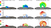 |
Fig. 5. Investigation of the flux rope eruption mechanisms. The top row shows the field lines colored based on the scaled NLFFF coefficient, the middle row the decay index and the bottom row the twist number (see the text for the explanation). The results are shown from left to right for initializing the zero-β MHD simulation with the TMFM snapshot at t−24, t−12, and tref. The bottom part of the figures shows the magnetogram, which is the bottom boundary of our simulations. The results are shown here only for the 1.5 × Ωopt. In the bottom right panel the subdomain enclosing the main flux system is indicated by the black box. |
In the left panels, the CWsin curves for all the cases (both the whole simulation and the subdomain V2 as well as for Ωopt and 1.5 × Ωopt) show similar trends. Overall, the TMFM simulation evolves towards a more force-free state after an initial nonforce-free phase which coincides with the rapid emergence of the active region into the simulation. For an extended period of time starting at approximately September 4, 2017 21:00, CWsin shows only minor variations around a value of ∼0.13 for the subdomain. The subdomain has slightly lower values of CWsin than the whole domain while the free magnetic energy attains higher values for the 1.5 × Ωopt case. The whole simulation domain showing larger CWsin (i.e., being more nonforce-free) is likely because the extended domain includes nonforce-free structures not directly related to the active region dynamics such as current sheets. The free magnetic energies in the whole domain (solid black curve) and in the subdomain (dashed black curves) show a similar, relatively monotonously, increasing trend throughout the simulation. It is notable that the degree to which the magnetic field is force-free in the subdomain is roughly equivalent at all three initialization times as well and for both the TMFM runs (Ωopt as well as 1.5 × Ωopt). However, for the entire domain, the CWsin metric shows a clear departure for the 1.5 × Ωopt case at the reference time. Thus, that magnetic field configuration is less force-free in the areas outside the active region as compared to all other cases.
The right panels show the corresponding evolution of CWsin in the zero-β MHD simulations for all investigated initialization times and for both Ωopt and 1.5 × Ωopt cases as well as for the whole box (solid lines) and the subdomain (dashed lines). Again, the CWsin values for the subdomain are smaller than for the whole simulation box. There are no consistent or significant variations in the level of how force-free the field is between different initialization times in particular early in the simulation and for the subdomain, except for the 1.5 × Ωopt reference time case noted above. It it also notable that the simulation initiated 24 hours prior to the reference time shows a comparable level of force-freeness even though the simulation is less dynamic as shown previously.
4.4. Analyzing the decay index and twist
To investigate the mechanism underlying the dynamics, we compute three parameters, namely, the force-free coefficient α, the twist number Tw of the magnetic field and the decay index n. As mentioned in Sect. 1, both the kink and torus instability have been suggested as the eruption mechanism of the investigated flux rope previously in the literature, both of which can be evaluated using the quantities mentioned above.
The results of this analysis are shown in Fig. 5 for the initial configurations of the zero-β simulations initialized using the TMFM output at t−24 (left columns), t−12 (middle columns) and the reference time (right columns). The results are shown here only for the 1.5 × Ωopt.
The top row of the figure shows field lines color-coded by the nondimensional quantity αL where α is the scalar relating the current density and magnetic field in a force-free magnetic field configuration ∇ × B = αB and L is a length scale (arbitrarily) chosen to be 1 Mm. Here, the parameter was evaluated by computing α = μ0J ⋅ B/B2.
For a strictly force-free field, α is constant along a field line. For the three snapshots, most of the shown field lines are close to a force-free state, as any clear variation in the color along a field line is not discernible. This is consistent with the results in Sect. 4.3, where it was found that the field is relatively close to a force-free state. The clearest departures are the field lines close to the null point where abrupt changes in α are visible especially for the two later snapshots.
The middle row of Fig. 5 shows the decay index n that quantifies the rate of the decay of the overlying magnetic field with height computed as
 (11)
(11)
where Bex = |Bex| represents the magnitude of the external magnetic field overlying the magnetic flux rope. When the FR is located in a region where the decay index exceeds a critical value, typically n ≳ 1.5, the magnetic field surrounding the FR decays sufficiently fast with height so that the FR may be subject to the torus instability causing it to erupt (e.g., Zuccarello et al. 2015; Kliem & Török 2006).
To compute the decay index, we approximated the external magnetic field with a potential magnetic field computed using periodic conditions on the lateral boundaries and Neumann boundary conditions on the bottom boundary so that in each simulation the potential magnetic field, and therefore decay index, is constant in time throughout the MHD evolution. We use all components of the potential magnetic field in the computation, with minor differences when employing other choices.
The middle row of Fig. 5 shows that the investigated zero-β MHD simulations begin with similar relative distributions with low values close to the photosphere and values increasing towards the top. For all investigated cases, the MHD simulation starts with a situation where the field lines pass through the regions where the critical value of the decay parameter is exceeded (n = 1.5). However, for the reference run, the value of the decay parameter is clearly the highest and exceeds the critical value in a region that is clearly the largest. In contrast, the simulation initiated at t−24 only in certain locations exceeds the critical value.
The bottom row shows the twist number defined as
 (12)
(12)
where J∥ denotes the component of the current density parallel to the magnetic field and the integral is computed along a given field line. The twist number indicates the number of turns a magnetic field line winds around a neighboring field line that is infinitesimally close by. We note that for a force-free field, Tw = ∫FLα/4π ds.
For the initial state at t−24, the shown field lines have a considerably smaller (in absolute value) twist as compared to the two later initialization times (Tw > −0.5). In particular the t−12 initial configuration contains a bundle of field lines with a twist value |Tw|> 1, often taken as an indication of the presence of a flux rope. Similar high values are no longer visible at the reference time for the shown field lines.
5. Discussion
In the previous section, we presented the results of initiating a zero-β MHD simulation of AR 12673 using the magnetic field configuration provided by a time-dependent magnetofrictional model. The TMFM model, driven by photospheric electrograms determined through an inversion process from the vector magnetogram observations, evolves the magnetic field over a period of several days capturing the build up of magnetic energy and helicity. In contrast, the MHD simulation employs a line-tied photospheric boundary condition suitable for modeling the dynamic evolution over relatively short timescales.
Our approach of linking TMFM and zero-β MHD raises the question whether the eruption of the flux systems is due to the change of governing equations and numerical schemes or driven by the nature of the phenomena. To address this the zero-β simulation was initiated at three distinct instances of time separated by 12 h with the latest (reference time) corresponding close in time to that of the eruptive X9.3 flare observed in the AR on September 6, 2017 at 11:53 UT. As shown, we find that using the TMFM results employing the optimized electrograms (Ωopt), the magnetic field configuration 24 h prior to the reference time is stable. In contrast, the model initiated at the reference time exhibits a flux system that evolves monotonically towards the upper corona. The simulation at the intermediate initialization time exhibits similar characteristics as the reference time run time but the rise was slightly at a lower rate. These clear differences in the evolution of the flux systems confirm that the outcome of the simulation depends on the snapshot it was initiated with rather than the transformation of the model from TMFM to MHD. The initiation of the MHD simulation with the TMFM run using an electrogram with 1.5 times the optimized value (1.5 × Ωopt) resulted in considerably faster rise of the tracked flux bundles. In particular, the case initialized with the reference time reached the top of the simulation box before the mid-point of the simulation. Unlike for the optimized electrogram, for the 1.5 × Ωopt case also the run initialized 24 hours before the reference time produced a twisted flux system that rose towards the upper corona. These results are consistent with the results of Kumari et al. (2023) who found that increasing the magnitude of the parameters controlling the noninductive electric field resulted in the magnetic field configuration exhibiting eruptive behavior at increasingly earlier times.
To investigate in more detail the differences in the evolution of the flux systems in the different simulations Fig. 6 shows snapshots of the MHD simulation initiated 12 h before the reference time from the optimized electrogram TMFM run at three different times during the simulation (t = 0, t = 200, t = 600 s). Two flux systems with different magnetic connectivity are depicted using white-purple and rainbow-colored field lines, drawn from photospheric locations indicated by A and B, respectively. Initially, the two flux systems are not connected, and so the regions A and B are not magnetically connected, with field lines originating from them instead connecting to the opposite polarity regions close to the main PIL of the AR. As the MHD simulation progresses, the evolution of the field configuration of the two systems features a sharp change in their connectivity resulting in the two flux systems sharing common foot points as the field lines increasingly connect between regions A and B thereby adding flux to the rising flux rope. This change in connectivity for both systems is mediated by the null point indicated by the red arrow in panel c. At the photospheric level, the foot points of the field lines move rapidly along the boundary with the movement indicated by the yellow arrows in panel b. This movement takes place despite the fixed density and zero velocity boundary condition. These are features of slip-running reconnection (Aulanier et al. 2006; Janvier et al. 2013) where the connectivity between nearby magnetic field lines changes in a continuous manner resulting in their slipping movement. In the MHD simulation, the movement is asymmetric, with the field lines of the white-purple system traversing a significantly greater distance along the photosphere than the rainbow-colored field lines. In this simulation, the subsequently rising flux rope is largely formed via this process, and thus contributes in a key fashion to the eruptive dynamics of the flux system. Slip-running reconnection has also been observationally shown, in another event, to be an important process in eruptive solar flares (e.g., Jing et al. 2017).
 |
Fig. 6. Evolution of two initially unconnected flux systems forming the rising flux rope via slip-running reconnection in the MHD simulation initiated at t−12. An animated version of this image is provided online. |
It is noteworthy that the slip-running reconnection does not take place to the same extent in the MHD simulation initiated 24 h prior to the reference time. To understand the reason for this difference, Fig. 7 depicts the initial states of the MHD simulations initialized 12 and 24 h before the reference time for the TMFM simulation using the optimized electrograms. In addition to the flux systems in the vicinity of the PIL, the images show an isocontour (magenta surface) of the magnitude of the magnetic field. The figure shows a distinct difference in the magnetic field structures. At t−24, the blue-yellow field lines show that the magnetic field exhibits a fan-spine-like topology. The outer spine is visible as a horn-like structure by the isocontour, and indicated by the yellow arrow in panel a. The spine terminates at the null point indicated by the red arrow. In contrast, at t−12, the magnetic field is characterized by an isolated null point. This is visible as an isolated closed contour indicated by the red arrow in panel b. The presence of the fan-spine topology effectively shields the null point from the white-purple and rainbow-colored flux systems at t−24, whereas at t−12 they have more direct access which enables the slip-running reconnection to proceed. We speculate that this difference in topology is the main reason for the flux system to be stable in the t−24 run.
 |
Fig. 7. Visualization of the field line topology in the vicinity of the null point. The partly transparent magenta surface shows an isocontour of |B| = 0.003 T. Panel (a) shows the configuration at t−24 while (b) at t−12. |
The role of the detailed evolution of the photospheric flux distribution in triggering the flare events has been discussed in previous works. In Bamba et al. (2020), the importance of the intrusion of the eastern negative polarity region (centered at approximately (x, y) = (−20, 0) Mm in Fig. 2) into the positive polarity region is highlighted. Based on the observed emission and magnetic field modeling, an interpretation of the evolution of the magnetic connectivity during the events is presented (see Fig. 9 in Bamba et al. 2020). The overall evolution in our simulation, as described in the previous sections, is consistent with their schematic. For example, the change in connectivity of the negative polarity region to the northwest (region B in Fig. 6, denoted F1 in Bamba et al. 2020) with the northern part of the main polarity inversion line takes place in our simulation in a similar fashion. In our simulation, the progression happens precisely as a result of the slip-running reconnection. However, in our simulation this dynamics takes place already earlier, several hours before the intrusion of the negative polarity region has started. Thus, while our results are similar in terms of the progression of the change in connectivity during the event, we do not find the intrusion to be crucial for the change in the connectivity after the event has been triggered.
The dynamics of the magnetic field at different times of the event were also studied using MHD simulations by Inoue & Bamba (2021). Similar to our results, the coronal magnetic field in their simulation is unstable resulting in an eruptive event well before the observed event, six hours before the X2.2 flare. At this earlier time, Inoue & Bamba (2021) report the dynamics in the simulation to be triggered due to reconnection at a more distant null point (denoted null point B in their Fig. 9). Interestingly, this null point appears to be in the same location and having a similar magnetic topology as the horn-like structure in our results (see Fig. 7). However, at time t−24, in our model the topology in this region is of a fan-spine type, which eventually forms into the isolated null visible in our model at t−12.
As discussed in the Introduction, NOAA AR 12673 show-cased here was previously studied by many authors with different approaches (NLFFF extrapolation, data-driven TMFM, etc.) who proposed torus (Inoue & Bamba 2021) or kink instabilities as the eruption mechanisms. To further investigate this matter we computed the twist number and decay index in all three initialization snapshots used in the ideal zero-β MHD simulations. According to Kliem et al. (2004), if the twist value exceeds a critical number of 3.5π, which is about 1.75 rotations about the axis the FR may be susceptible to the kink instability. The flux rope investigated here has negative twist values. In the MHD simulation initialized at t−24, the Tw values were relatively close to zero. For the t−12 case in turn the field lines were more twisted and the critical threshold was approached at the bottom of the flux system, while for the reference time run the field lines were highly twisted but clearly not close to the critical value. The decay index in turn exceeded the critical threshold for torus instability (> 1.5) for all cases, in particular so for the reference time. Care needs to be taken, however, in interpreting these results as all investigated field lines may not be part of the actual flux rope. As the twist values were the largest in the run initiated 12 h before the reference time, while the reference time run showed the largest decay index and the largest area exceeding the critical value, it is therefore likely that torus instability played a key role in this event, with the decay of the overlying field propelling the flux rope in the reference time simulation.
6. Conclusion
The goal of this work was to model eruptive coronal magnetic fields by initiating an ideal zero-β MHD simulation using a more realistic and dynamically evolved magnetic configuration compared to data-constrained and static approaches such as NLFFF extrapolation. This magnetic field was produced through the data-driven and time-dependent magnetofrictional model (TMFM) which allows magnetic energy and helicity to build up using the data-driven process in a computationally inexpensive model compared with MHD simulation. The TMFM snapshots at three different times were used as the input to the MHD model. We also produced the snapshots using two different sets of TMFM runs with different electrograms reflecting different amounts of energy injection into the corona.
The linking of the models was tested with AR 12673 that was seen at the center of the solar disk on September 3, 2017 and released several big flares and CMEs. The most notable one, which this study focuses on, was an X9.3 class flare that occurred on September 6, 2017 at 11:53 UT. The reference initiation time matched the time of the X-class flare and the other two times were 12 and 24 h before this time. The linked TMFM and zero-β MHD model successfully produced an erupting flux rope in all except one investigated case. In the simulation initialized 24 h before the reference time, and with less helicity injected in the TMFM simulation, only a small twisted flux system formed that did not erupt. The likely cause was a fan-spine magnetic structure shadowing the null point and preventing the on-set of the slip-like magnetic reconnection, detected to occur in other runs. For the other investigated cases the dynamical evolution of the tracked flux bundles was dependent on the initialization time and the injected helicity. In the case where the initiation was carried out close to the eruption time and more energy and helicity was injected into the system the flux rope rose fastest and reached the top of the simulation while for other cases where the eruption was observed the tracked flux bundles rose slower and stayed within the simulation box. The overall change in magnetic field topology during the event was found to be consistent with previous interpretations based on observational analysis. However, the intrusion of the negative polarity region, discussed in previous works, was not found to be crucial as the eruptive dynamics in the simulation occurred before the intrusion. Instead, the dynamics appear consistent with previous dynamical modeling results which also produce an eruption well before the observed event due to the influence of a distant null point.
The linked model also allowed probing the cause of the eruption by calculating the decay index and twist number, suggesting that the torus instability would have played a role in the eruption. The results of this study suggest that using TMFM as input to an MHD model is a viable approach for simulating the dynamics of solar eruptions in a manner that combines computational efficiency and a realistic description of the eruptive coronal fields. Nevertheless, our MHD simulation was simplified. The linked model can be improved in the future, in particular by including a more accurate thermodynamic description of the plasma.
Movie
Supplementary material provided by the author(s).
Movie 1 associated with Fig. 6 Access Supplementary Material
Acknowledgments
All authors acknowledge the ERC under the European Union’s Horizon 2020 Research and Innovation Programme Project SolMAG 724391. J.P. and F.D. acknowledge the Academy of Finland Project 343581. All authors acknowledge the Finnish Centre of Excellence in Research of Sustainable Space (Academy of Finland grant numbers 312390, 312357, 312351 and 336809).
References
- Aulanier, G., Pariat, E., Démoulin, P., & Devore, C. R. 2006, Sol. Phys., 238, 347 [NASA ADS] [CrossRef] [Google Scholar]
- Ballegooijen, A. A. V., Priest, E. R., & Mackay, D. H. 2000, ApJ, 539, 983 [NASA ADS] [CrossRef] [Google Scholar]
- Bamba, Y., Inoue, S., & Imada, S. 2020, ApJ, 894, 29 [NASA ADS] [CrossRef] [Google Scholar]
- Chen, J. 2017, Phys. Plasmas, 24, 090501 [Google Scholar]
- Chertok, I. M., Belov, A. V., & Abunin, A. A. 2018, Space Weather, 16, 1549 [NASA ADS] [CrossRef] [Google Scholar]
- Cheung, M. C. M., & DeRosa, M. L. 2012, ApJ, 757, 147 [NASA ADS] [CrossRef] [Google Scholar]
- Chitta, L. P., Kariyappa, R., Ballegooijen, A. A. V., Deluca, E. E., & Solanki, S. K. 2014, ApJ, 793, 112 [NASA ADS] [CrossRef] [Google Scholar]
- Guo, Y., Xia, C., Keppens, R., Ding, M. D., & Chen, P. F. 2019, ApJ, 870, L21 [NASA ADS] [CrossRef] [Google Scholar]
- Hoilijoki, S., Pomoell, J., Vainio, R., Palmroth, M., & Koskinen, H. E. J. 2013, Sol. Phys., 286, 493 [NASA ADS] [CrossRef] [Google Scholar]
- Hou, Y. J., Zhang, J., Li, T., Yang, S. H., & Li, X. H. 2018, A&A, 619, A100 [NASA ADS] [CrossRef] [EDP Sciences] [Google Scholar]
- Inoue, S. 2016, Progr. Earth Planet. Sci., 3 [CrossRef] [Google Scholar]
- Inoue, S., & Bamba, Y. 2021, ApJ, 914, 71 [CrossRef] [Google Scholar]
- Inoue, S., Magara, T., Pandey, V. S., et al. 2014, ApJ, 780, 101 [Google Scholar]
- Inoue, S., Kusano, K., Büchner, J., & Skála, J. 2018a, Nat. Commun., 9, 174 [NASA ADS] [CrossRef] [Google Scholar]
- Inoue, S., Shiota, D., Bamba, Y., & Park, S.-H. 2018b, ApJ, 867, 83 [CrossRef] [Google Scholar]
- Inoue, S., Hayashi, K., Miyoshi, T., Jing, J., & Wang, H. 2023, ApJ, 944, L44 [NASA ADS] [CrossRef] [Google Scholar]
- Janvier, M., Aulanier, G., Pariat, E., & Démoulin, P. 2013, A&A, 555, A77 [NASA ADS] [CrossRef] [EDP Sciences] [Google Scholar]
- Jiang, C., Zou, P., Feng, X., et al. 2018, ApJ, 869, 13 [NASA ADS] [CrossRef] [Google Scholar]
- Jiang, C., Bian, X., Sun, T., & Feng, X. 2021, Front. Phys., 9, 224 [NASA ADS] [Google Scholar]
- Jing, J., Liu, R., Cheung, M. C. M., et al. 2017, ApJ, 842, L18 [NASA ADS] [CrossRef] [Google Scholar]
- Kilpua, E. K. J., Balogh, A., von Steiger, R., & Liu, Y. D. 2017, Space Sci. Rev., 212, 1271 [CrossRef] [Google Scholar]
- Kliem, B., & Török, T. 2006, Phys. Rev. Lett., 96, 255002 [Google Scholar]
- Kliem, B., Titov, V. S., & Török, T. 2004, A&A, 413, L23 [NASA ADS] [CrossRef] [EDP Sciences] [Google Scholar]
- Kumari, A., Price, D. J., Daei, F., Pomoell, J., & Kilpua, E. K. J. 2023, A&A, 675, A80 [NASA ADS] [CrossRef] [EDP Sciences] [Google Scholar]
- Liu, L., Cheng, X., Wang, Y., et al. 2018, ApJ, 867, L5 [Google Scholar]
- Lumme, E., Pomoell, J., & Kilpua, E. K. J. 2017, Sol. Phys., 292, 191 [CrossRef] [Google Scholar]
- Metcalf, T. R., De Rosa, M. L., Schrijver, C. J., et al. 2008, Sol. Phys., 247, 269 [Google Scholar]
- Morosan, D. E., Carley, E. P., Hayes, L. A., et al. 2019, Nat. Astron., 3, 452 [Google Scholar]
- Pagano, P., Mackay, D. H., & Poedts, S. 2013, A&A, 554, A77 [NASA ADS] [CrossRef] [EDP Sciences] [Google Scholar]
- Pariat, E., Leake, J. E., Valori, G., et al. 2017, A&A, 601, A125 [CrossRef] [EDP Sciences] [Google Scholar]
- Pomoell, J., Vainio, R., Kissmann, R., et al. 2008, Sol. Phys., 253, 249 [Google Scholar]
- Pomoell, J., Lumme, E., & Kilpua, E. 2019, Sol. Phys., 294, 41 [NASA ADS] [CrossRef] [Google Scholar]
- Price, D. J., Pomoell, J., Lumme, E., & Kilpua, E. K. J. 2019, A&A, 628, A114 [NASA ADS] [CrossRef] [EDP Sciences] [Google Scholar]
- Romano, P., Elmhamdi, A., & Kordi, A. S. 2019, Sol. Phys., 294, 4 [Google Scholar]
- Schuck, P. W., & Antiochos, S. K. 2019, ApJ, 882, 151 [Google Scholar]
- Török, T., Kliem, B., & Titov, V. S. 2004, A&A, 413, L27 [NASA ADS] [CrossRef] [EDP Sciences] [Google Scholar]
- Török, T., Temmer, M., Valori, G., et al. 2013, Sol. Phys., 286, 453 [CrossRef] [Google Scholar]
- Verma, M. 2018, A&A, 612, A101 [NASA ADS] [CrossRef] [EDP Sciences] [Google Scholar]
- Webb, D. F., & Howard, T. A. 2012, Liv. Rev. Sol. Phys., 9, 3 [Google Scholar]
- Welsch, B. T. 2018, Sol. Phys., 293, 113 [Google Scholar]
- Yan, X. L., Wang, J. C., Pan, G. M., et al. 2018, ApJ, 856, 79 [NASA ADS] [CrossRef] [Google Scholar]
- Yang, S., Zhang, J., Zhu, X., & Song, Q. 2017, ApJ, 849, L21 [NASA ADS] [CrossRef] [Google Scholar]
- Zou, P., Jiang, C., Feng, X., et al. 2019, ApJ, 870, 97 [NASA ADS] [CrossRef] [Google Scholar]
- Zou, P., Jiang, C., Wei, F., et al. 2020, ApJ, 890, 10 [Google Scholar]
- Zuccarello, F. P., Aulanier, G., & Gilchrist, S. A. 2015, ApJ, 814, 126 [Google Scholar]
- Zuccarello, F. P., Pariat, E., Valori, G., & Linan, L. 2018, ApJ, 863, 41 [Google Scholar]
All Figures
|
Fig. 1. Snapshots of the zero-β MHD simulation showing the evolution of the multiflux system preceding the September 6, 2017 flare and its accompanying CME eruption. The top and third rows show the initial situation for the simulations (t = 0) and the second and bottom rows the simulations at time t = 600 s. The left panels give results when the zero-β MHD simulation was initialized with the TMFM snapshot at time t−24, i.e., 24 h before the reference time, while the right panels show the results when the initialization was made at the reference time (September 6, 2017 at 09:24 UT). The two top panels give the results when the TMFM simulation was performed with the optimized Ω and the bottom rows when it was performed with 1.5 times the optimized Ω. The color of the field lines were selected in order to facilitate the visual distinguishability of the flux systems. |
| In the text | |
|
Fig. 2. Change of the maximum height of field lines rooted in the photosphere at time t = 600 s compared to their initial height, Δh = h(t = 600)−h(t = 0). Panels from left to right show the result for the simulations initialized at t−24, t−12 and the reference time, respectively, using Ωopt. The orange solid (black dashed) contour indicates field lines of lengths 100 (200) Mm. The gray scale shows the vertical component of photospheric magnetic field saturated at ±0.1 T. |
| In the text | |
|
Fig. 3. Parametric evolution of the zero-β MHD simulation. The panels show: a) the apex altitude of the main flux rope, b) the ratio of the free to total magnetic energy, c) kinetic energy, and d) the slab magnetic energy as a function of simulation time (in seconds) in the zero-β MHD simulation. The black curve shows the run where the MHD simulation was initialized with the TMFM snapshot at the reference time, and the purple (green) curves the case where the simulations were initialized 24 (12) h before the reference time. The solid curves show the results for the optimized Ω and the dashed lines for the 1.5 × optimized Ω. The tracking is continued until the boundary effects start to take over when the flux rope approaches the top of the simulation box (case for the reference time run with 1.5 × Ωopt), see the text for details. |
| In the text | |
|
Fig. 4. Comparison of force-freeness and free magnetic energy in the TMFM and zero-β MHD simulations. Left panels: evolution of CWsin force-freeness factor during TMFM simulation of the entire computational box (blue) and a box enclosing the main flux rope (orange). The black curves show the evolution of free magnetic energy for the whole domain (solid curve) and the subdomain (dashed curve). The reference time (black), and times 12 (green) and 24 (purple) h before the reference time are shown by dashed vertical lines. Right panels: time evolution of CWsin in the zero-β MHD simulation for the whole domain (solid) and subdomain (dashed). The top panels show the results for the optimized Ω and the bottom panels for the 1.5 × optimized Ω. |
| In the text | |
|
Fig. 5. Investigation of the flux rope eruption mechanisms. The top row shows the field lines colored based on the scaled NLFFF coefficient, the middle row the decay index and the bottom row the twist number (see the text for the explanation). The results are shown from left to right for initializing the zero-β MHD simulation with the TMFM snapshot at t−24, t−12, and tref. The bottom part of the figures shows the magnetogram, which is the bottom boundary of our simulations. The results are shown here only for the 1.5 × Ωopt. In the bottom right panel the subdomain enclosing the main flux system is indicated by the black box. |
| In the text | |
|
Fig. 6. Evolution of two initially unconnected flux systems forming the rising flux rope via slip-running reconnection in the MHD simulation initiated at t−12. An animated version of this image is provided online. |
| In the text | |
|
Fig. 7. Visualization of the field line topology in the vicinity of the null point. The partly transparent magenta surface shows an isocontour of |B| = 0.003 T. Panel (a) shows the configuration at t−24 while (b) at t−12. |
| In the text | |
Current usage metrics show cumulative count of Article Views (full-text article views including HTML views, PDF and ePub downloads, according to the available data) and Abstracts Views on Vision4Press platform.
Data correspond to usage on the plateform after 2015. The current usage metrics is available 48-96 hours after online publication and is updated daily on week days.
Initial download of the metrics may take a while.