| Issue |
A&A
Volume 683, March 2024
|
|
|---|---|---|
| Article Number | A79 | |
| Number of page(s) | 16 | |
| Section | Stellar structure and evolution | |
| DOI | https://doi.org/10.1051/0004-6361/202345888 | |
| Published online | 08 March 2024 | |
Confirmation of the presence of a CRSF in the NICER spectrum of X 1822-371
1
Dipartimento di Fisica e Chimica – Emilio Segrè, Università di Palermo, via Archirafi 36, 90123 Palermo, Italy
e-mail: rosario.iaria@unipa.it
2
INAF/IASF Palermo, via Ugo La Malfa 153, 90146 Palermo, Italy
3
Department of Physics, University of Trento, Via Sommarive 14, 38122 Povo (TN), Italy
4
Dipartimento di Fisica, Università degli Studi di Cagliari, SP Monserrato-Sestu, KM 0.7, Monserrato 09042, Italy
Received:
11
January
2023
Accepted:
28
December
2023
Aims. X 1822-371 is an eclipsing binary system with a period close to 5.57 h and an orbital period derivative Ṗorb of 1.42(3) × 10−10 s s−1. The extremely high value of its Ṗorb is compatible with a super-Eddington mass transfer rate from the companion star and, consequently, an intrinsic luminosity at the Eddington limit. The source is also an X-ray pulsar, it shows a spin frequency of 1.69 Hz and is in a spin-up phase with a spin frequency derivative of 7.4 × 10⁻¹² Hz s−1. Assuming a luminosity at the Eddington limit, a neutron star magnetic field strength of B = 8 × 10¹⁰ G is estimated. However, a direct measure of B could be obtained observing a CRSF in the energy spectrum. Analysis of XMM-Newton data suggested the presence of a cyclotron line at 0.73 keV, with an estimated magnetic field strength of B = (8.8 ± 0.3)×1010 G.
Methods. Here we analyze the 0.3–50 keV broadband spectrum of X 1822-371 combining a 0.3–10 keV NICER spectrum and a 4.5–50 keV NuSTAR spectrum to investigate the presence of a cyclotron absorption line and the complex continuum emission spectrum.
Results. The NICER spectrum confirms the presence of a cyclotron line at 0.66 keV. The continuum emission is modeled with a Comptonized component, a thermal component associated with the presence of an accretion disk truncated at the magnetospheric radius of 105 km and a reflection component from the disk blurred by relativistic effects.
Conclusions. We confirm the presence of a cyclotron line at 0.66 keV inferring a NS magnetic field of B = (7.9 ± 0.5)×1010 G and suggesting that the Comptonized component originates in the accretion columns.
Key words: eclipses / ephemerides / stars: individual: X 1822-371 / stars: neutron / X-rays: binaries
© The Authors 2024
 Open Access article, published by EDP Sciences, under the terms of the Creative Commons Attribution License (https://creativecommons.org/licenses/by/4.0), which permits unrestricted use, distribution, and reproduction in any medium, provided the original work is properly cited.
This article is published in open access under the Subscribe to Open model. Subscribe to A&A to support open access publication.
1. Introduction
The low-mass X-ray binary system (LMXB) X 1822-371 (4U 1822-37) is a persistent eclipsing source with an orbital period of 5.57 h, hosting an accreting X-ray pulsar with a spin frequency close to 1.69 Hz (Jonker & van der Klis 2001) and in a spin-up phase with a derivative of  Hz s−1 (Mazzola et al. 2019). X 1822-371 belongs to the class of accretion disc corona (ADC) sources (White & Holt 1982), with an inclination angle between 81° and 84° (Heinz & Nowak 2001). The distance to this source was estimated to be between 2–2.5 kpc by Mason & Cordova (1982) using infrared and optical observations. The 0.1–100 keV unabsorbed luminosity is 1.2 × 1036 erg s−1, adopting a distance of 2.5 kpc (Iaria et al. 2001b). Recently, using Gaia data, Arnason et al. (2021) estimated a distance to X 1822-371 of
  kpc, which implies that the observed luminosity should be a factor by six larger than that estimated in the literature.
The most recent orbital ephemeris of the source X 1822-371 was reported by Anitra et al. (2021), who suggested that the orbital period derivative is Ṗorb = (1.42 ± 0.03) × 10−10 s s−1 adopting a quadratic ephemeris. This high orbital period derivative cannot be explained by a conservative mass transfer at the accretion rate inferred from the observed source luminosity. A highly non-conservative mass transfer is needed at a rate up to seven times the Eddington limit for a neutron star (NS) mass of 1.4 M⊙ (see Burderi et al. 2010; Bayless et al. 2010; Iaria et al. 2011; Mazzola et al. 2019). In this scenario, the intrinsic luminosity produced by the source is likely at the Eddington limit (a few 1038 erg s−1), two orders of magnitude higher than the observed luminosity of 1036 erg s−1.
Assuming the neutron star (NS) is in spin equilibrium, Jonker & van der Klis (2001) showed that the NS magnetic field is close to B ≃ 8 × 10¹⁰ G for an intrinsic luminosity of 1038 erg s−1 while B ≃ 2 × 10¹⁶ G for an intrinsic luminosity of 1036 erg s−1. Finally, they suggested a B value close to 1012 G, discussing the spectral models reported in the literature up to that time, which yields an intrinsic luminosity of the source of 1037 erg s−1 given the measured Ṗpulse/Ppulse value.
However, a direct measure of the magnetic field strength B is possible only by observing a cyclotron resonance scattering feature (CRSF) in the spectrum. Sasano et al. (2014), studying the Suzaku broadband spectrum of X 1822-371, suggested the presence of a CRSF at 33 keV and a corresponding value of B ≃ 3 × 10¹² G. Iaria et al. (2015) showed that the B-value proposed by Sasano et al. (2014) is not consistent with the spin-up regime of the source. By studying the XMM spectrum of X 1822-371, Iaria et al. (2015) identified a possible CRSF at 0.73 keV corresponding to a value of B = (8.8 ± 0.3)×1010 G. The authors suggested that the observed Comptonized component could be produced in the accretion column onto the NS magnetic caps, and estimated a magnetospheric radius of ∼250 km.
Iaria et al. (2013) suggested a geometry of the source consisting of an optically thick corona close to the neutron star identified by a Comptonization component in the source spectrum and an optically thin extended corona with an optical depth of τ = 0.01. The optically thin corona was introduced for three reasons: 1) since the intrinsic luminosity is at the Eddington limit while the observed one is a hundred times weaker, an optically thin extended corona with τ = 0.01 would scatter along the line of sight one percent of the intrinsic luminosity (the source is observed with an edge-on geometry); 2) the optically thin corona must be extended because the observed eclipses are partial; 3) the NS spin pulsation is observed. If the corona were extended and optically thick, the pulsation would be diluted by photon scatterings in the corona while assuming the existence of an optically thin corona with τ = 0.01 the travel time of the photons through the optically thin corona (≃2 s) is comparable to the spin period (≃0.59 s) and part of the pulsed photons can reach the observer after scattering.
Bak Nielsen et al. (2017) proposed that the seed-photons spectrum (composed of a blackbody component plus a power law with a cut-off energy at 10 keV and photon index Γ = 1) is scattered by an extended optically thin corona with an optical depth ranging from 0.01 to 3. According to the authors, their model eliminates the optically thick Comptonizing region and explains the system only with an optically thin (or moderately thick; τ ≃ 0.01 − 3) corona surrounding the X-ray pulsar.
Recently, Anitra et al. (2021) showed that the broadband X-ray spectrum of the source can be fitted with a model composed of: a thermal component associated with an accretion disk emission, a Comptonized component and a reflection component from the accretion disk. The emission from the central region of the system is obscured from direct view by the outer edge of the disk. However, it is scattered along the line of sight by an optically thin corona with optical depth of 0.01.
In this work, we analyze the broadband spectrum of X 1822-371 combining a NICER spectrum with an exposure time of 11 ks and NuSTAR spectrum with an exposure time of 96 ks. We confirm the presence of a cyclotron absorption line close to 0.7 keV by taking advantage of the large effective area of NICER between 0.5 and 2 keV. We confirm that the model discussed by Anitra et al. (2021) fits the broadband spectrum well and suggest that the Comptonizing corona is placed at the accretion column over the magnetic caps of X 1822-371.
2. Observations and data analysis
Neutron Star Interior Composition Explorer (NICER, Gendreau et al. 2016) observed X 1822-371 on 2022 Jun 04 for a total exposure time of 11 ks (obsid. 5202780101). The primary instrument of NICER is the X-ray Timing Instrument (XTI), which is an array of 56 photon detectors that operate in the 0.2–12 keV energy range. We reduced the NICER data using the pipeline tool nicerl2 in NICERDAS v10 available with HEASOFT v6.31 and adopting the standard filters; the used calibration database version was xti20221001. During the observation the Focal Plane Modules (FPM) 63 and 43 were noisy; the tool nicerl2 rejected all the events collected by FPM 63 and generated GTIs for FPM 43 after data screening. In order to create the spectrum, we utilized the nicerl3-spect tool to exclude FPM 14 and 34 due to elevated detector noise. The 3–10 keV light curve was extracted using the tool nicerl3-lc. The source spectrum and the scorpeon background file were extracted using the tool nicerl3-spect and setting the options bkgformat=file. We added the systematic error suggested by the NICER calibration team to the spectrum1, and grouped the data using the ftool ftgrouppha applying an optimal rebinning grouptype=optmin to have at least 25 counts per energy bin (groupscale=25, Kaastra & Bleeker 2016).
NuSTAR observed X 1822-371 from 2022 February 15 at 08:21:09, to February 17 at 14:26:19 (ObsID 30701025002), with a duration of 200 ks and a total exposure time of 96 ks. To produce the light curve, the source and the background spectra of FPMA and FPMB, we utilized the Nupipeline and Nuproducts scripts in HEASOFT. A circular region with a radius of 100 arcsec was chosen to extract the events from the source. The background events were extracted from a circular region within the field of view (FOV) that is devoid of source photons. This circular region was selected from the same detector where the source is located and has a radius of 100 arcsec. After checking that the FPMA and FPMB spectra are similar in the 4–50 keV energy band we summed the two spectra using the ftool addspec2, the summed spectrum was rebinned as done for the NICER spectrum.
2.1. Update of the orbital ephemeris
We produced the NuSTAR light curve extracting the FPMA events in the 5–40 keV energy range and applying the barycentric corrections to the event arrival times using the ftool barycorr.
We folded the light curve, adopting a reference epoch Tfold = 59625 MJD and a reference period of Pfold = 0.2321107 days (see Fig. 1). To estimate the eclipse arrival time Tecl we used the procedure proposed by Burderi et al. (2010) finding Tecl = 59625.19445(48) MJD/TDB. Adopting a reference orbital period of P0 = 0.232109571 days and a reference eclipse time T0 = 50353.08728 MJD, we found that the number of orbital cycles N is 39947 and the delay associated with the eclipse arrival time is 2259(41) s. To update the orbital ephemeris, we included the eclipse arrival time shown above with those reported by Mazzola et al. (2019) and Anitra et al. (2021). The delays as a function of orbital cycles reveal that the source exhibits stable expansion over 44 years of data (see top panel of Fig. 2).
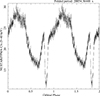 |
Fig. 1. NuSTAR/FPMA folded light curve assuming as epoch Tfold = 59625 MJD and an orbital period of 0.2321107 days. The period is divided into 512 bins. For clarity, two orbital phase cycles are shown. |
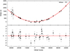 |
Fig. 2. Delays vs. orbital cycles for the quadratic ephemeris (top panel). We used the eclipse arrival times shown by Mazzola et al. (2019; see Table 1 in their work), the one obtained by Anitra et al. (2021) and that shown in the text. Residuals in units of σ (bottom panel). |
We fitted the delays as a function of cycles adopting the quadratic model y = a + bN + cN2, where a = ΔT0 is the correction to the adopted T0, b = ΔP is the correction to the adopted P0 and c = 1/2P0Ṗ allows us to estimate the orbital period derivative Ṗ. We obtained a χ2(d.o.f.) of 47(32) (similarly to what obtained by Mazzola et al. 2019). The best-fit quadratic curve (red) and the corresponding residuals in units of σ are shown, respectively, in the top and bottom panels of Fig. 2.
The updated orbital ephemeris are:
where the first and the second term represent the refined values of the reference epoch T0, orb and orbital period P0, orb, respectively. The third term allows us to estimate an orbital period derivative of Ṗorb = 1.426(26) × 10−10 s s−1.
We added a cubic term in order to test the presence of a second derivative of the orbital period. By fitting the delays with a cubic function we found a χ2(d.o.f.) of 43(31), that is the addition of a cubic term is not statistically significant (σ ∼ 1.3).
Finally, we verified whether a gravitational quadrupole coupling produced by tidal dissipation (Applegate & Shaham 1994) could be detectable in our data as done by Mazzola et al. (2019). To this aim, we added a sinusoidal term to the quadratic model (hereafter LQS model). By fitting the delays with the LQS model we obtained a χ2(d.o.f.) of 34(29), indicating that the addition of the sinusoidal term is not statistically significant with a detection of 2σ.
The folded NuSTAR/FPMA light curve, imposing as null phase the passage at the eclipse and adopting the orbital period at the times of the observation, is shown in Fig. 3 (black curve).
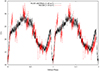 |
Fig. 3. 5–40 keV NuSTAR/FPMA folded light curve (black curve) and 3–10 keV NICER folded light curve (red curve). The folded light curves have 512 bins per peiod, each bin corresponds to 39.17 s. |
We applied the barycentric correction to the 3–10 keV NICER light curve using the ftool barycorr and folded it using the eclipse arrival time (Te = 59734.51859 MJD/TDB) and the orbital period predicted by the ephemeris shown in Eq. (1) (Porb = 20054.36448 s). We show the folded light curve in Fig. 3 (red curve), the orbital modulation of the two light curves is similar along the orbital period.
2.2. Spin-period search
We searched for the NS spin frequency in the 5–40 keV NuSTAR/FPMA light curve binned at 0.01 s. We corrected the event arrival times for the binary orbital motion using a sin i = 1.006(5) lt-s (Jonker & van der Klis 2001), the eclipse arrival time shown above and the orbital period at the time of the observation.
We used the ftool efsearch of the XRONOS package, adopting the start time of the observation as reference time and a resolution of the period search of 10−6 s. We explored around a period of 0.591116 s, estimated using Eq. (2) in Mazzola et al. (2019), and subsequently, we fitted the peak of the corresponding χ2 curve with a Gaussian function. We assumed that the centroid of the Gaussian function is the best estimate of the spin period. We found that the spin period is 0.591124781 s, the χ2 peak associated with the best period is 135 (see the left panel in Fig. 4), and the probability of obtaining a χ2 value greater than or equal to the χ2 peak by chance, having 15 degrees of freedom, is 2.2 × 10⁻²¹ for a single trial. Considering the 1000 trials in our research, we expect almost 2.2 × 10⁻¹⁸ periods with a χ2 value greater than or equal to χ2 peak. This implies a detection significance with σ ≃ 8.7.
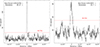 |
Fig. 4. Folding search for periodicity in the 5–40 keV NuSTAR/FPMA light curve of the obsid. 30701025002 (left panel) and obsid. 30301009002 (right panel). The horizontal dashed line indicates the χ2 value of 34.72 at which we have the 99.73% confidence level for a single trial, corresponding to a significance of 3σ. |
At the light of this result we searched for the spin period in the NuSTAR obsid. 30301009002 discussed by Anitra et al. (2021). The FPMA light curve was rebinned at 0.01 s and we selected the events in the 5–40 keV energy range. After applying the barycentric correction to the event arrival times we corrected them for the orbital motion adopting the eclipse arrival time of Tecl = 58234.1536(5) MJD/TDB (see Anitra et al. 2021) and the orbital period at the time of the observation. Using the ftool efsearch, we explored around a period Pspin of 0.591472 s obtaining a spin period of 0.59145871 s. The χ2 peak associated with the best period is 59 (see the right panel in Fig. 4), and the probability of obtaining a χ2 value greater than or equal to the χ2 peak by chance, with 15 degree of freedom, is 3.7 × 10⁻⁷ for a single trial. Considering the 1000 trials in our research, we expect almost 3.7 × 10⁻⁴ periods with a χ2 value greater than or equal to the χ2 peak. This implies a detection significance with σ ≃ 3.4.
Finally, we searched for periodicity in the NICER data without success. We searched in the 2–10 keV and 5–10 keV energy band because the pulse amplitude increases with increasing energy, it is less than 0.5% between 2 and 6 keV and less than 1% between 6 and 10 keV (see Jonker & van der Klis 2001). We believe that the low effective area of NICER above 5 keV and the short exposure time prevent us from finding a statistically significant signal.
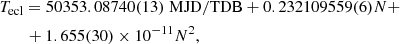
We refined the long-term spin period derivative using the spin period best-values, which span 25 yrs, shown in Table 1. We fitted the Pspin values with a linear function (see the top panel of Fig. 5) and associated the post-fit errors to the parameters. We found a dependence of Pspin on time given by:

where the time t is given in MJD and the spin period derivative is ̇Pspin = −2.64(2)×10−12 s s−1 (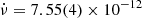 Hz s−1) confirming that X1822-371 is spinning up. Propagating the errors on the Pspin from Eq. (2) and using the eclipse arrival times from the two NuSTAR observations, we obtained the errors on the Pspin. We found that Pspin = 0.59112(2) s and Pspin = 0.59144(2) s for the NuSTAR observations taken in 2022 and 2017, respectively.
Log of the spin periods.
Fluctuations are present in the data (see bottom panel in Fig. 5) as already discussed by Bak Nielsen et al. (2017) although the decreasing trend is evident. We show the pulse profiles in Fig. 6. By fitting with a sinusoidal function we found that the pulse amplitude is 1.8% for both the observations. Finally, we note that the pulse profiles are not perfectly sinusoidal and their shape is similar to that shown by Jonker & van der Klis (2001) for the energy band 9.4–22.7 keV.
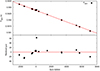 |
Fig. 5. Long-term spin period change (top panel) and corresponding residuals in units of μs. The linear decrease of the pulse period over time suggests that the NS is in a spin-up regime. |
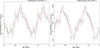 |
Fig. 6. 5–40 keV NuSTAR/FPMA folded light curve of the obsid. 30701025002 (left panel) and obsid. 30301009002 (right panel). The curves are folded to have 16 bins per period. Two periods are shown fro clarity. The red curves represent the best-fit model using a sinusoidal function. |
2.3. The NICER spectrum
Initially, we fitted only the NICER spectrum in the 0.3–10 keV energy band with XSPEC v12.13.0c. We adopted the TBabs component accounting for the ISM abundances (Wilms et al. 2000) and set the photoelectric cross section reported by Verner et al. (1996). We adopted a model composed of a Comptonized component (Comptb in XSPEC, Farinelli et al. 2008) and two Gaussian emission lines at 6.4 keV and 6.96 keV. We kept fixed the parameter log A at the value of 8 in the Comptb component. The parameter log A is called the illumination factor, where 1/(1 + A) is the fraction of the seed-photon radiation directly seen by the observer, whereas A/(1 + A) is the fraction upscattered by the Compton cloud. By fixing log A = 8 we are assuming that all the seed-photons are upscattered. Hence, the adopted model is ModelA: TBabs*(Comptb+gauss+gauss); this simple model does not give a good fit of the spectrum; we found a χ2(d.o.f.) value of 453(144). To improve the fit we added a blackbody component (bbodyrad in XSPEC) to the model (ModelB: TBabs*(bbodyrad+Comptb+gauss+gauss)) finding a χ2(d.o.f.) value of 258(142). The fit is still statistically unsatisfactory, since large residuals are present below 1 keV, where the data-to-model ratio is larger than 5% (see top panel in Fig. 7).
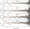 |
Fig. 7. 0.3–10 keV ratios for Models B, C, D and F. The systematic error is that suggested by the NICER calibration team. The red horizontal lines indicate a deviation of the model from the data of 2%. |
A possible explanation for those residuals below 1 keV is that there might be abundances of oxygen and/or iron deviating from solar values. Therefore, we replaced the photoelectric absorption model Tbabs with the Tbfeo model, allowing the oxygen and iron abundances to vary3. We fitted the spectrum adopting ModelC: TBfeo*(bbodyrad+Comptb+gauss+gauss). We obtained a χ2(d.o.f.) value of 113(140), the abundances of oxygen and iron were 3.6 ± 0.4 and > 10 times the solar abundances, respectively. Regardless of the plausibility of the abundance values associated with oxygen and iron, we still notice that the ratio exhibits residuals larger than 5% around 0.7 keV (see the second panel from the top in Fig. 7).
We replaced the Tbfeo component in the model with Tbabs and added two absorption edges (edge in XSPEC) with threshold energies fixed at 0.56 keV and 0.71 keV. The two absorption edges are associated with the neutral K-shell O and neutral L-shell Fe. This choice implies that the neutral iron abundance estimated by the edge at 0.71 keV is different from that estimated by the neutral iron K-shell edge at 7.1 keV with Tbabs component, making the model non-self-consistent. The sole purpose of this model is to address the residuals below 1 keV. We fitted the spectrum with ModelD: TBabs*edge*edge(bbodyrad+Comptb+gauss+gauss). We found a χ2(d.o.f.) value of 99(140). The ratio corresponding to this model is shown in the third panel from the top in Fig. 7. We observe that close to 0.7 keV the model deviates from the data by 5%. Since the introduced systematic error is less than 2%, we conclude that this model, besides being non-self-consistent, fails in its purpose of accurately modeling the spectrum below 1 keV.
To take into account a potential misrepresentation of the solar wind charge exchange (SWCX) background during the observation we fitted the spectrum adopting ModelE: TBpcf*TBabs*(gaOK+gaNe9+Comptb+gauss+gauss), where the components gaOK and gaNe9 are two Gaussian emission lines with energy fixed at 0.53 keV and 0.92 keV and associated with neutral oxygen and Ne IX, respectively. Initially, we let the widths of the two lines free to vary and obtained a χ2(d.o.f.) value of 116(138). However, the best-fit values of the widths of the K-shell O and the Ne IX lines are 60 ± 15 eV and  eV; the broadening of the two lines suggests that the Gaussian components try to fit the continuum emission. In fact, SWCX lines are typically modeled as delta functions (see e.g., Fujimoto et al. 2007), so this model must be rejected. Then, we fitted the spectrum keeping fixed the widths of the gaOK and gaNe9 components at 5 eV (hereafter ModelF). We found a χ2(d.o.f.) value of 136(140) but large residuals persist below 1 keV as shown in the bottom panel of Fig. 7.
Moreover, we investigated the possibility that the residuals below 1 keV are due to a poor modeling of the SCORPEON background spectrum. Therefore, we extracted the source spectrum and the background model (using the nicerl3-spect tool and setting bkgformat=script) to simultaneously fit the source spectral model and the SCORPEON background model4. To fit the source spectrum and background together we adopted the pgstat statistic. However, the fit in the 0.3–15 keV energy range leaves the broad residuals below 1 keV unchanged with a ratio larger than 4%, suggesting that the residuals observed at 0.7 keV are not related to a mismodeling of the background.
Before proceeding with the investigation of the X 1822-371 spectrum below 1 keV, we note that the models from C to F (summarized in Table 2) show a reduced χ2 less than 1 but the corresponding data-to-model ratios exceed 5% below 1 keV (see Fig. 7). The reduced χ2 values should not lead to the conclusion that we found a good fit because they are influenced by the systematic error we added to the spectrum. On the other hand, ratios exceeding 2% below 1 keV indicate the need to add an additional component to obtain a good fit of the spectrum below 1 keV5.
Adopted models to fit the NICER spectrum.
Analyzing a XMM-Newton observation of X 1822-371, Iaria et al. (2015) suggested the presence of a cyclotron line at 0.7 keV, and we decided to investigate this scenario. We added to Model B a gabs component at 0.7 keV to take into account the possible presence of a cyclotron line. (hereafter ModelG: gabs*TBabs*(bbodyrad+Comptb+gauss+gauss)). We obtained a χ2(d.o.f.) value of 85(139) with a Δχ2 of 172.9 with respect to ModelB and the residuals below 1 keV disappear. We show the unfolded model and the corresponding ratio in Fig. 8, the best fit values of the parameters associated with this model are shown in the third column of Table 3.
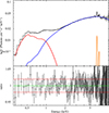 |
Fig. 8. 0.3–10 keV unfolded spectrum using Models G (top panel); the blackbody, the Comptonized component and the emission lines at 6.4 keV and 6.96 keV are shown with the red, blue and orange colors, respectively. The corresponding data-to-model ratio is in bottom panel. |
Best-fit values of the parameters associated with Model G.
To verify whether the gabs component at 0.7 keV is statistically significant we used Monte-Carlo simulations as shown by Bhalerao et al. (2015). We adopted ModelB as our null hypothesis and simulated 1000 fake spectra. Then we fitted each fake spectrum with ModelB and ModelB plus gabs (i.e. ModelG) annotating the Δχ2 value obtained for the addition of gabs. Since the cyclotron line adds three free parameters, we expect that the histogram of Δχ2 values follows a χ2 distribution with three degrees of freedom. We show the results in Fig. 9.
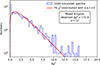 |
Fig. 9. Monte-Carlo simulations results for testing the gabs significance for Model B. The blue histogram shows Δχ2 values obtained in the simulations, and the red curve is a χ2 distribution with 3 d.o.f. The Δχ2 = 172.9 attained in actual data is significantly higher than values attained in simulations (by ∼12σ). |
The highest Δχ2 obtained in our simulation is 15.8, significantly lower than Δχ2 = 172.9 obtained in real data. From our simulation the probability to observe a Δχ2 of 172.9 by chance is 7.8 × 10⁻³⁵ that corresponds to a significance of ∼12σ.
We repeated the same procedure for Model C, D and F. We show the observed Δχ2 due to the addition of the gabs component and its statistical significance in the fourth and fifth column of Table 2. The addition of the gabs component to the tested models is always larger than 3 sigmas except for Model D for which we find the significance is only 0.1σ. So, except for Model D, the addition of a gabs component significantly improves the quality of the fit.
2.4. Combined fit of the NICER spectra
To further investigate the possible presence of overabundances of neutral oxygen and neutral iron with respect to the solar-abundances values, that is Model C and Model D, we combined the aforementioned NICER spectrum with five additional NICER spectra obtained from five different pointings of the source.
The five NICER observations (obsid. from 5202780102 to 5202780106) have an exposure time of 1.4 ks, 4.3 ks, 5.9 ks, 2.4 ks and 1.7 ks, respectively. The observations were conducted from June 23 to June 26, 2022. During the observation the Focal Plane Module (FPM) 63 was noisy, and during the screening of the data the tool nicerl2 rejected all the events collected by FPM 63. Moreover, in order to produce the spectrum we removed FPM 14 and 34 using nicerl3-spect tool because of increased detector noise.
The source spectrum and the scorpeon background file were extracted using the tool nicerl3-spect and setting the options bkgformat=file. We added the systematic error suggested by the NICER calibration team to the spectrum and grouped the data using the ftool ftgrouppha by applying an optimal rebinning grouptype=optmin to have at least 25 counts per energy bin (groupscale=25, Kaastra & Bleeker 2016).
To fit the six spectra we included to the analyzed models a constant component (const) to account for flux variations of the source in different observations. Additionally, we left the blackbody normalization and the temperature of the seed photons (kTs) free to vary for all six spectra. Finally, we added an edge at 2.1 keV to address the calibration feature at 2 keV present in the NICER spectra (see Fig. 8).
Initially, we fitted the six spectra using Model B. We found a χ2(d.o.f.) of 1219(844). Below 1 keV, the model deviates from the data by 10%, as shown in the top-left panel of Fig. 10. By adding a gabs component at 0.7 keV we obtained a χ2(d.o.f.) of 594(841) and a Δχ2 of 625. We show the ratio corresponding to this model in the bottom-left panel of Fig. 10, the residuals below 1 keV disappear.
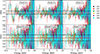 |
Fig. 10. Data-to-model ratio of the six NICER (0.3–10 keV) spectra with respect to the different adopted models, with or without the gabs component. The adopted colors for each spectrum are shown in the legend in which we indicate the last three digits of the corresponding observation ObsId. In the top panels we show the ratio corresponding to Model B, Model C, and Model D, respectively. In the bottom panels we show the ratio of the same models including a gabs component at 0.7 keV. The black horizontal lines indicate a deviation of the model from the data corresponding to 2%. |
To verify whether the gabs component at 0.7 keV is statistically significant we used Monte-Carlo simulations. We adopted ModelB as our null hypothesis and simulated 1000 fake spectra. We show our simulations is the left panel of Fig. 11, the largest value of Δχ2 obtained from the simulations is 23.2 that is significantly smaller than Δχ2 = 625 obtained in real data. The probability to observe a Δχ2 of 625 by chance is 1.6 × 10−132 corresponding to 24.5σ. The best-fit parameters of the gabs component are E = 0.726 ± 0.008 keV, σ = 0.106 ± 0.012 keV and Strength . We conclude that the addition of the gabs component to Model B is highly significant.
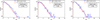 |
Fig. 11. Monte-Carlo simulation results to assess the statistical significance of adding the gabs component into Model B, Model C, and Model D. The addition of the gabs component is significant at 24.5σ, 6.6σ, and 9.8σ in Model B, Model D, and Model C, respectively. |
By fitting the data using Model D We found a χ2(d.o.f.) of 657(842). The depths of the edges at 0.56 keV and 0.71 keV are 0.31 ± 0.03 and 0.20 ± 0.02, respectively. Below 1 keV, the model deviates from the data by at least 5%, as shown in the top-center panel of Fig. 10. Adding a gabs component at 0.7 keV we obtained a χ2(d.o.f.) of 592(839) and a Δχ2 of 65. We show the ratio corresponding to this model in the bottom-center panel of Fig. 10, the residuals below 1 keV disappear. The depth of the edge at 0.56 keV and 0.71 keV are < 0.17 and < 0.12, respectively. The best-fit parameters of the gabs component are  keV, σ = 0.09 ± 0.02 keV and Strength = 0.04 ± 0.02.
Similarly, we assessed the statistical significance of incorporating the gabs component in this instance. We adopted ModelD as our null hypothesis and simulated 1000 fake spectra. We show our simulations in the center panel of Fig. 11, the largest value of Δχ2 obtained from the simulations is 15.7 that is smaller than Δχ2 = 65 obtained in real data. The probability to observe a Δχ2 of 65 by chance is 2.1 × 10⁻¹¹ corresponding to 6.6σ. We conclude that the addition of the gabs component to Model D is highly significant.
Finally, we fitted the six NICER spectra adopting ModelC, where we adopted the Tbfeo component leaving free to vary the O and Fe abundance. We found a χ2(d.o.f.) of 713(842); the abundances of O and Fe are 3.4 ± 0.2 and 11.5 ± 1.3 times the corresponding solar-abundance values. However, the ratio in the top-right panel of Fig. 10 shows that the model deviates from data by at least 5% below 1 keV. By adding to the model a gabs component at 0.7 keV we obtained a χ2(d.o.f.) of 594(839) and a Δχ2 of 119. We show the ratio corresponding to this model in the bottom-right panel of Fig. 10, the residuals below 1 keV disappear. The abundances of O and Fe are 0.8 ± 0.5 and  times the corresponding solar-abundance values. The best-fit parameters of the gabs component are
 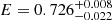 keV,
keV, 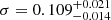 keV and Strength = 0.07 ± 0.03.
Likewise, we evaluated the statistical significance associated with the inclusion of the gabs component in this case. We adopted ModelC as our null hypothesis and simulated 1000 fake spectra. We show our simulations is the right panel of Fig. 11, the largest value of Δχ2 obtained from the simulations is 17.2 that is smaller than Δχ2 = 119 obtained in real data. The probability to observe a Δχ2 of 119 by chance is 5.7 × 10⁻²³ corresponding to 9.8σ. We conclude that the addition of the gabs component to Model C, is highly significant. So, the inclusion of the gabs component is always necessary in models B, C, and D, as the addition of this component exhibits a significance exceeding 5 sigma for all the three examined models.
2.5. Combined fit of the NICER spectrum with two XMM/EPIC-pn spectra
To further enhance the robustness of our detection of the cyclotron line at 0.7 keV and to better investigate whether there are two edges associated with the K-shell of neutral oxygen and the L-shell of neutral iron below 1 keV, we reanalyzed two XMM/EPIC-pn spectra combining them with the NICER spectrum.
The obsid. 0784820101 was already analyzed by Anitra et al. (2021). The authors analyzed the EPIC-pn spectrum in the 2–10 keV energy band suggesting calibration issues in the spectrum associated with the presence of a silicon edge at 1.8 keV. The source was observed by the XMM-Newton observatory on 2017 March 3 for a duration of 69 ks. During the observation the EPIC-pn camera was operating in Timing Mode. We reduced the XMM-Newton data using the Science Analysis Software (SAS) v21.0.0. Initially, we extracted the EPIC-pn events between 10 and 12 keV to verify the presence of particle flaring background6. The light curve shows a strong flaring activity after the first 30 ks from the beginning of the observation. To mitigate the effects of particle flaring, we selected the time intervals with a rate lower than 1.5 c s−1 in the energy range 10–12 keV.
We show the source and background EPIC-pn light curve in the 0.6–10 keV energy range cleaned from the particle flaring background in Fig. 12 (left panel). The source light curve clearly shows the orbital modulation and ranges between 40 c s−1 and 90 c s−1, two partial eclipses are present at 14 000 s and 34 000 s from the beginning of the observation.
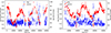 |
Fig. 12. 0.6–10 keV EPIC-pn light curve (source in red, background in blue) corresponding to the obsid. 0784820101 (left panel) and obsid. 0111230101 (right panel). Bin time 100 s. |
The EPIC-pn spectrum and background were extracted selecting RAWX between 26 and 47 and RAWX between 3 and 5, respectively. The EPIC-pn spectrum has an exposure time of 41 ks, it was grouped using the ftool ftgrouppha by applying an optimal rebinning grouptype=optmin to have at least 25 counts per energy bin (groupscale=25, Kaastra & Bleeker 2016). To fit the data, we adopted the range of 0.6–10 keV for the EPIC-pn spectrum.
The obsid. 0111230101 was already analyzed by Iaria et al. (2015); the authors suggested the presence of an absorption line, discussed as cyclotron absorption line, close to 0.7 keV by analyzing the EPIC-pn and RGS spectra in the 0.6–10 keV and 0.35–2 keV energy band, respectively. The observation was carried out on 2001 March 7 for a duration of 54 ks. During the observation the EPIC-pn camera was operating in Timing Mode. We reduced the XMM-Newton data using the Science Analysis Software (SAS) v21.0.0.
To mitigate the effects of particle flaring background, we selected the time intervals with a rate lower than 1.5 c s−1. We show the source and background EPIC-pn light curve in the 0.6–10 keV energy range cleaned from the particle flaring background in Fig. 12 (right panel). The source light curve shows the orbital modulation and ranges between 30 c s−1 and 70 c s−1, two partial eclipses are present close to 20 000 s and 40 000 s from the beginning of the observation.
The EPIC-pn spectrum and background were extracted selecting RAWX between 31 and 44 and RAWX between 3 and 5. The EPIC-pn has an exposure time of 41 ks, it was grouped as shown above.
The two XMM observations are distant in time, we produced the hardness ratios (HRs) using the energy band 0.6–2 keV and 2–10 keV to check a possible change in the shape spectrum. The HRs are shown in Fig. 13. We observe that the HR value is approximately 2 for the observation carried out in 2001 and approximately 1.7 for the one carried out in 2017.
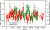 |
Fig. 13. EPIC-pn hardness ratios of the XMM observation made in 2001 (green color) and in 2017 (red color). The bin time is 100 s. |
Since the NICER spectrum alone may suggest that the addition of two edges at 0.56 and 0.71 keV does not require the presence of an additional cyclotron line at 0.7 keV although we note that the data-to-model ratio below 1 keV is approximately 5%, we decide to verify that this continues to be true when we perform a combined fit of the NICER and the two EPIC-pn spectra. At 0.7 keV, the effective area of EPIC-pn is approximately 900 cm2, which is only 30% lower than that of NICER, which is around 1250 cm2. Given that the NICER spectrum has a systematic error larger than 1% and an exposure time of 11 ks, while both EPIC-pn spectra have an exposure time of 41 ks, we can compare the statistics of the three spectra at 0.7 keV without the risk of biasing the fit toward the NICER spectrum.
Initially, we fitted the NICER spectrum (0.3–10 keV), the 0.6–10 keV EPIC-pn spectrum corresponding to obsid. 0784820101 (hereafter PN1 spectrum), the 0.6–10 keV EPIC-pn spectrum corresponding to obsid. 0111230101 (hereafter PN2 spectrum) using Model B, to which we added a Gaussian component in the Fe-K region of the spectrum because PN1 and PN2 spectra require it. We added a constant to accommodate the different normalization between the three spectra. The constant value was held fixed at 1 for the NICER spectrum, while it was allowed to vary for PN1 and PN2 spectra. To take into account the systematic feature present close 2 keV in the NICER spectrum (see Fig. 8) we added an absorption edge with energy threshold fixed at 2.1 keV; we kept fixed to zero the depth of the edge for the other spectra. In addition, since the three spectra were extracted from non-simultaneous observations, we allowed the normalization of the blackbody component, the seed-photon temperature and the energy index α of the Comptb component to vary independently. We forced the value of the electronic temperature of the PN1 spectrum to that of the NICER spectrum. We left to vary independently the energies and the normalizations of the two narrow Gaussian line at 6.4 and 6.96 keV for PN1 spectrum and kept fixed at 70 eV their widths. Finally, we added two Gaussian emission lines at PN1 and PN2 spectrum at 1.18 keV and 1.343 keV with width fixed at 5 eV. To take into account of the systematic at 2 keV in the PN2 spectrum we added a Gaussian component with null width and negative normalization (hereafter we call this model Model H).
By fitting the spectrum, we obtained an unacceptable fit with a χ2(d.o.f.) of 1337(359), the ratio below 1 keV shows that the model deviate of 20% from the data (top-left panel of Fig. 14). Then, we added to model a gabs component at 0.7 keV (hereafter Model I). The best-fit improves significantly; we found a χ2(d.o.f.) of 494(356) with a Δχ2 = 843. The ratio is within 2% as shown in the bottom-left panel of Fig. 14. The best-fit parameters are shown in the third column of Table 4. The best-fit parameters of the gabs component are E0 = 0.728 ± 0.005 keV, σ0 = 0.097 ± 0.008 keV and Strength = 0.059 ± 0.009, these results are consistent with those obtained by fitting the NICER spectrum alone.
 |
Fig. 14. Ratios combining the 0.3–10 keV NICER (black), PN1 (red) and PN2 (green) spectrum. In the top panels the residuals corresponding to Model I, Model L, and Model M removing the gabs component. In the bottom panels the residuals associated with the best-fit model shown in Table 4. The orange horizontal lines indicate a deviation of the model from the data larger than 2%. |
To test the significance of adding the gabs component, we simulated 1000 spectra using the Monte-Carlo method as described in the previous section. The histogram of the Δχ2 values obtained from the simulation is shown in the left panel of Fig. 15 and it is well-fitted by a χ2 with three d.o.f. (red curve). We found that the largest value of Δχ2 obtained from the simulation is 15.9, the probability to observe a Δχ2 of 849 by chance is 5.2 × 10−180 corresponding to a statistical significance of 29σ.
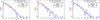 |
Fig. 15. Monte-Carlo simulation results to assess the statistical significance of adding the gabs component into Model I, Model L, and Model M. The addition of the gabs component is significant at 29σ, 10.5σ, and 12σ in Model I, Model L, and Model M, respectively. |
We started from Model H adding to it two absorption edges at 0.56 keV and 0.71 keV. By fitting the three spectra we found a χ2(d.o.f.) of 615(357), the data deviate from the model up to 5% below 0.6 keV as shown in the top-center panel of Fig. 14. We added to the model a gabs component at 0.7 keV (hereafter Model L). The best-fit improves significantly; we found a χ2(d.o.f.) of 484(354) with a Δχ2 = 131. We show the residuals in the bottom-center panel of Fig. 14. The best-fit parameter are shown in the fourth column of Table 4. The best-fit parameters of the gabs component are 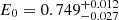 keV, σ0 = 0.075 ± 0.013 keV and Strength
 , these results are consistent with those obtained by adopting Model I.
Best-fit parameters combining PN1, PN2 and NICER spectra.
Also for this model, we assessed the significance of adding the gabs component as done previously. The histogram of the simulated spectra is shown in the middle panel of Fig. 15. We found that the largest value of Δχ2 obtained from the simulation is 16.7, the probability to observe a Δχ2 of 131 by chance is 8.6 × 10⁻²⁶ corresponding to a statistical significance of 10.5σ. Our test indicates that the addition of a component representing a cyclotron line at 0.7 keV is necessary, even though two edges are included in the model at 0.56 and 0.71 keV.
Finally, instead of adding two edges at 0.56 and 0.71 keV we used a self-consistent absorption model. Specifically, we replaced TBabs with TBfeo, allowing the abundances of oxygen and iron to vary freely, as suggested by the NICER team. By fitting the spectra we found a χ2(d.o.f.) of 658(357); also in this case the data deviate from the model up to 5% below 0.6 keV (top-right panel of Fig. 14). We added to the model a gabs component at 0.7 keV (hereafter Model M). We found a χ2(d.o.f.) of 489(354) with a Δχ2 = 169. The best-fit parameters are shown in the fifth column of Table 4, the residuals in the bottom-right panel of Fig. 14). The best-fit parameters of the gabs component are  keV,
keV,  keV and Strength
 , these results are consistent with those obtained by adopting Model I and Model L. In this case, we find that the largest value of Δχ2 obtained from the simulation is 17.2, the probability to observe a Δχ2 of 169 by chance is 5.2 × 10⁻³⁴ corresponding to a statistical significance of 12σ (right panel of Fig. 15).
Since the component associated with a 0.7 keV cyclotron line is required for all three described models, we discuss a model that requires a cyclotron line at low energies, with abundances of O and Fe fixed to solar values (Model G) in the subsequent sections of the work.
However, since the reduced-χ2 associated with the NICER spectrum alone is much smaller than one and attributable to an overestimation of systematic errors in the 0.3–10 keV range (see the third column in Table 3), we extracted the spectrum by assigning a 1% systematic error to our data. Fitting the NICER spectrum adopting Model G, we obtained a χ2 of 117(138) with the ratio between 0.3 and 10 keV below 2%. The best-fit values shown in the fourth column of Table 3 indicate that the spectral shape remains unchanged when transitioning from the systematic error suggested by the NICER calibration team to a 1% systematic error, while the reduced-χ2 increases from 0.61 to 0.87.
2.6. Combined NICER-NuSTAR spectra
We fitted the combined 0.3–10 keV NICER spectrum and the 4–50 keV NuSTAR spectrum using Model G where we left free to vary the parameter log A of the Comptb component. To take into account the systematic feature present close 2 keV in the NICER spectrum (see Fig. 8) we added an absorption edge with energy threshold fixed at 2.1 keV; we kept fixed to zero the depth of the edge for the NuSTAR spectrum. In addition, since the two spectra are extracted from non-simultaneous observations, we allowed the energy index α of the Comptb component to vary independently between the two spectra. We added a constant to account for the different normalization between the two spectra. The constant value was kept fixed at 1 for the NICER spectrum, while it was free to vary for the NuSTAR spectrum. Finally, we kept fixed at 70 eV the widths of the two lines in the Fe-K region.
Fitting the spectrum, we obtained an unacceptable fit with a χ2(d.o.f.) of 1038(324). In the NuSTAR spectrum, a feature at 9.6 keV is evident, which we modeled with an absorption edge. We set the depth of the edge to zero for the NICER spectrum. The addition of the absorption edge improves the fit; we obtained a χ2(d.o.f.) of 905(322). However, large residuals were still present in the Fe-K region of the spectrum. For this reason, we added an additional Gaussian component to the model. The model (hereafter Model1) is:

We found a χ2(d.o.f.) value of 469(319), the added Gaussian emission line has a centroid of 6.13 ± 0.08 keV and a σ of 730 ± 90 eV. To better constrain this broad line, we left the width of one of the two narrow lines free to vary and constrained the amplitude of the second narrow line to vary with the first one. The obtained fit was statistically equivalent; we found a χ2(d.o.f.) of 469(318). The best-fit parameters are reported in the third column of Table 5, the corresponding residuals are shown in the bottom-left panel of Fig. 16. Analyzing the residuals, it is evident that the NuSTAR spectrum (in red) is not well modeled above 15 keV. We added a power-law component with a cut-off at low energies to fit the residuals at high energies. We fixed the energy of the cut-off component (expabs in XSPEC) to the seed-photon temperature of the Comptb component. The model (hereafter Model2) is:
Best-fit parameters combining NICER and NuSTAR spectra.

where po indicates the power-law component.
By adding the absorbed power-law component we obtained a χ2(d.o.f.) of 302(316) and the residuals above 15 keV disappeared. We show the best-fit parameters in the fourth column of Table 5, the unfolded spectrum and the residuals are show in the top-left and middle-left panel of Fig. 16.
 |
Fig. 16. Unfolded spectrum of Model 2 (top-left panel) using a 0.3–10 keV NICER/XTI spectrum (black color) combined with a 4–50 keV NuSTAR/(FPMA+FPMB) spectrum (red color), the colors of the components are described in the text. Residuals adopting Model 2 and adopting Model 1 are shown in the middle-left panel and bottom-left panel, respectively. Unfolded spectrum and residuals of Model 3 in top-right and bottom-right panel, respectively. |
In the unfolded spectrum we show the blackbody, the Comptonized component and the power-law in red, blue and green color, respectively. The narrow emission lines are in orange color and, finally, the broad Gaussian line is shown in magenta.
The temperature of the thermal emission is 0.173 ± 0.007 keV, the Comptonized component has a seed-photon temperature of 1.34 ± 0.05 keV, an electron temperature of 4.22 ± 0.07 keV, a α-index < 0.13 and 0.22 ± 0.06 for NICER and NuSTAR spectrum respectively. The log A parameter is 0.20 ± 0.10 implying that (39 ± 6)% of the seed photons is directly seen by the observer while the remaining part is scattered in the Comptonizing cloud. The narrow emission lines are at 6.39 ± 0.02 keV and 6.91 ± 0.03 keV with a width of  eV. The first line is associated with an emission line of neutral iron, the second line is marginally compatible with the presence of Fe XXVI ions.
The broad emission line has an energy of  keV and a width of
  eV. The photon-index of the power-law component is 1.96 ± 0.05. The gabs component at low energies, that is the cyclotron line, has a centroid at 0.724 ± 0.014 keV, a width of 0.10 ± 0.02 keV and an optical depth of 0.25 ± 0.10. Finally, an absorption edge at 9.62 ± 0.09 keV is observed.
The unabsorbed fluxes in the 0.1–100 keV energy range are 1.3 × 10⁻⁹ erg s−1 cm−2, 2.6 × 10⁻¹¹ erg s−1 cm−2 and 1.4 × 10⁻¹⁰ erg s−1 cm−2 associated with the Comptonized component, the blackbody and the power-law component, respectively. Assuming a distance to the source of 2.5 kpc, the total unabsorbed luminosity in the 0.1–100 keV energy range is 1.1 × 1036 erg s−1 (6.6 × 1036 erg s−1 for a distance to the source of 6.1 kpc, recently estimated by Arnason et al. (2021). Hereafter, we assume that the distance to the source is 6.1 kpc.
Following a scenario describing the presence of cyclotron line at 0.7 keV we changed the gabs component with a cyclabs component. We obtained a statistically equivalent fit with a χ2(d.o.f.) = 304(316); the best-fit values associated with the cyclabs component are: E = 0.69 ± 0.02 keV, width = 0.12 ± 0.03 keV and depth = 0.31 ± 0.04. These values are compatible with those reported by Iaria et al. (2015).
Because we are observing a broad Gaussian line in the Fe-K region of the spectrum we explored a scenario in which a reflection component from the accretion disk is present as suggested by Anitra et al. (2021). To model the spectrum we changed the broad Gaussian line with a reflection component blurred by relativistic effects. We assumed that the incident radiation comes from the Compton cloud. The model (hereafter Model 3) is:
where rfxconv is the component that takes into account the reflection component from the accretion disk while rdblur is the component that takes into account the relativistic blurring. We fixed the outer radius Rout at 3000 gravitational radii after checking that the χ2 value was not sensible to this parameter. The inclination angle was fixed at 82.5° as reported in literature (Mason & Cordova 1982).
We show the best-fit values in the fifth column of Table 5, the unfolded spectrum and the residuals are shown in the top-right and bottom-right panels of Fig. 16. In the unfolded spectrum of Model 3 the red, blue, magenta and green component are the blackbody, the Comptonized component, the reflection component and the power-law. The two narrow emission lines in the Fe-K region are in orange.
We obtained that χ2(d.o.f.) = 296(315). The reflection component has a reflection amplitude of  , an inner disk radius of
  gravitation radii and a ionization of the disk of log(
 . The best-fit values of the gabs component are E0 = 0.66 ± 0.03 keV, σ0 = 0.17 ± 0.03 keV and an optical depth τ0 = 0.4 ± 0.2.
The unabsorbed fluxes in the 0.1–100 keV energy range are 1.2 × 10⁻⁹ erg s−1 cm−2, 3.3 × 10⁻¹¹ erg s−1 cm−2, 1.4 × 10⁻¹⁰ erg s−1 cm−2 and 1.2 × 10⁻¹⁰ erg s−1 cm−2 associated with the Compton cloud, the blackbody component, the power-law component and the reflection component, respectively. The total unabsorbed luminosity in the 0.1–100 keV energy range is 6.6 × 1036 erg s−1 for a distance to the source of 6.1 kpc.
3. Discussion
Using the NuSTAR data (obsid. 30701025002), we updated the orbital ephemeris of X 1822-371 by adding one eclipse arrival time. We find a Ṗorb of 1.426(26)×10−10 s s−1, compatible with the values present in literature (see, e.g., Anitra et al. 2021). As discussed before, the addition of a cubic term or a sinusoidal term to the quadratic model does not improve significantly the fit.
We estimated the spin period of the source during the two NuSTAR observations discussed above and confirmed the presence of a linear long-term decrease of the spin period finding Ṗspin of −2.64(2)×10−12 s s−1, compatible with the value reported by Bak Nielsen et al. (2017).
The analyzed energy spectrum was obtained by combining the 0.3–10 keV NICER spectrum (obsid. 5202780101) with the 4.5–50 keV NuSTAR spectrum. The continuum emission is composed of a blackbody component plus a Comptonized component and a power-law component. The blackbody component has a temperature of 0.158 ± 0.011 keV; by assuming a distance to the source of 6.1 kpc we infer an emission radius of  km. The seed-photon temperature and the electron temperature of the Comptonized component are kT
 keV and kTe = 4.34 ± 0.07 keV, respectively. The illumination factor log A is 0.35 ± 0.12 and the α value, the energy index of the Comptonization spectrum, is
  and 0.35 ± 0.07 for NICER and NuSTAR spectrum, respectively. We find that the percentage of seed-photon radiation directly seen by the observer is 31 ± 6% suggesting that the Comptonizing corona is geometrically compact and does not completely surround the inner regions of the system. The seed-photon emission radius is 2.4 ± 0.2 km.
The gabs component is interpreted as cyclotron absorption line (see also Iaria et al. 2015), with a centroid energy of E0 = 0.66 ± 0.03 keV. The relation between the energy of the fundamental harmonic and the magnetic field strength is B12 = E0/(11.6) (1 − 0.295 m/R6)−1/2 G, where m is the NS mass in unit of solar masses and R6 is the NS radius in units of 106 cm. The NS mass was estimated to be between 1.61 ± 0.15 and 1.70 ± 0.13 M⊙ (Iaria et al. 2015). Assuming a NS radius of 10 km and the value of E0, we estimate that the magnetic field strength is B = (7.9 ± 0.5)×1010 G and B = (8.1 ± 0.5)×1010 for a NS mass of 1.61 ± 0.15 M⊙ and 1.70 ± 0.13 M⊙, respectively. These values of the magnetic field strength are compatible with the estimate done by Jonker & van der Klis (2001) who calculated a value of B ∼ 8 × 10¹⁰ G for a luminosity of the source of 1038 erg s−1. In the following we discuss our results for a NS mass of 1.61 M⊙ (similar results are obtained for a NS mass of 1.70 M⊙).
We observe the weakest magnetic field strength ever inferred from an electron cyclotron line. Since the formation of a cyclotron line requires that the magnetic field is B > (v/c)2Bcrit, where v/c is the velocity of electrons (in units of the speed of light) perpendicular to the field lines and Bcrit = 4.4 × 10¹³ G, we expect that the electron velocity component perpendicular to the field lines is of the order of 10% the speed of light to obtain a threshold value of B of the order of 8 × 10¹⁰ G.
To estimate the expected luminosity from the source we used the Ghosh & Lamb (1979) equation, which links the spin-period derivative, its magnetic field and its luminosity:

where I45 is the NS moment of inertia in units of 1045 g cm2, R6 is the NS radius in units of 106 cm, m is the NS mass in units of solar masses and P is the spin period of the source, that is, 0.591124781(13) s. The parameter n(ωs) is the dimensionless accretion torque that is a function of the fastness parameter ωs. When ωs < 0.95, we can use the following approximate expressions (Ghosh & Lamb 1979):
![$$ \begin{aligned}&n\approx 1.39\left\{ 1-\omega _{\rm s}\left[4.03\left(1-\omega _{\rm s}\right)^{0.173}-0.878\right]\right\} \left(1-\omega _{\rm s}\right)^{-1} ,\nonumber \\&\omega _{\rm s} \approx 1.35\; \mu _{30}^{6 / 7} M_{1}^{-2/7} \left(P L_{37}^{3 / 7}\right)^{-1}. \end{aligned} $$](/articles/aa/full_html/2024/03/aa45888-23/aa45888-23-eq99.gif)
Iaria et al. (2015) showed that ωs is between 0.063 and 0.083 for a NS mass of X 1822-371 between 1 and 3 M⊙. Assuming a magnetic field strength of B = (7.9 ± 0.5) × 1010 G, a NS mass of 1.61 M⊙, a NS radius of 10 km and a spin-period derivative Ṗspin of −2.64(2) × 10−12 s s−1 we infer an intrinsic luminosity of 1.5 × 1038 erg s−1 (corresponding to a mass accretion rate of 1.13 × 10⁻⁸ M⊙ yr−1) that is very close to the Eddington luminosity of ∼2 × 1038 erg s−1. The intrinsic luminosity is 20 times larger than the observed luminosity (6.6 × 1036 erg s−1). This discrepancy is likely due to the high inclination angle of the source, between 81° and 84° (see Iaria et al. 2013; Anitra et al. 2021) which causes the emission from the central part of the system to be obscured by the outer edge of the disk. Although the discrepancy between the intrinsic luminosity of the source and the observed luminosity has decreased for a source distance of 6.1 kpc, the scenario described above still holds true. As the ratio between intrinsic and observed luminosity is approximately 20, the optical depth of the ADC should be around 0.05. Therefore, the ADC remains optically thin, and all the previous conclusions remain unchanged.
The flux associated with the blackbody component corrected by a factor ∼20 gives a blackbody radius of  km and a seed-photon radius of 10.7 ± 0.9 km compatible with an emission coming from the NS. We hence associate the blackbody component to the emission from the accretion disk, its radius indicating the inner radius of the disk. We do not correct this value for the inclination angle since we assume that the optically thin corona covers the whole accretion disk. We infer the magnetospheric radius Rm using the formula in Sanna et al. (2017),

where G is the gravitational constant, M is the NS mass, μ the NS magnetic dipole moment, and Ṁ is the mass accretion rate. The factor ϕ is given by the following equation

(Sanna et al. 2017), where μ26, R6 and  are the NS magnetic moment in units of 1026 G cm3, the NS radius in units of 106 cm and the mass accretion rate in unit of 10−9 M⊙ yr−1. The mean molecular weight κ is 0.615 for fully ionized matter, while the parameter α for a standard Shakura–Sunyaev disk model is set to 0.1 (Shakura & Sunyaev 1973). Adopting a NS mass of 1.61 M⊙, a B-field strength of (7.9 ± 0.5)×1010 G and a NS radius of 10 km, we obtain that Rm = 105 ± 5 km, that is smaller than the inner radius of the accretion disk, as expected for an X-ray pulsar.
We observe a reflection component from the accretion disk with a ionization parameter of log , compatible with the value obtained by Anitra et al. (2021). This value implies a relatively low ionization state of matter in the disk; the iron line is dominated by the Fe I-XX Kα transition (Fabian et al. 2000). The inner radius at which the reflection component is produced is
  gravitational radii, that corresponds to
  km for a NS mass of 1.61 M⊙. This value is compatible with the inner radius of the accretion disk of
  km derived above.
The Comptonized component is associated with a optically-thick corona. By using Eq. (10) in Farinelli et al. (2008) we find that the optical depth τ is 24 and 17 for the NICER and NuSTAR spectrum assuming a spherical geometry and 12 and 8 assuming a slab geometry.
From these findings, we can conclude that although there is a magnetosphere in place and the matter being accreted is channeled along the magnetic field lines, a portion of the matter has sufficient kinetic energy to overcome the magnetic barrier imposed by the magnetosphere. As a result, this matter penetrates the magnetosphere (possibly due to Rayleigh-Taylor and Kelvin-Helmholtz instabilities) and falls directly onto the surface of the NS. This phenomenon is likely favored by the large accretion rate, reaching the Eddington limit, and the magnetic field being relatively weak with a strength of 7.9 × 10¹⁰ G.
We therefore suggest that the Comptonized component is formed at the accretion column onto the magnetic caps and the seed-photons come from all the NS surface, in agreement with the observation that 31% of the seed-photons do not interact with the Comptonized region.
If we assume that the broadening of the cyclotron line (σ0 = 0.17 ± 0.03 keV) has thermal origin, we estimate a temperature of 13 keV not consistent with the electron temperature of 4.3 keV obtained from the fit. A possible explanation is that we are observing a gradient of the B-field strength along the accreting column. In this hypothesis we can infer the height of the column considering that the magnetic dipole moment μ = BR3 does not change, and then −ΔB/B = 3ΔR/R. By imposing ΔB as the sigma of the gabs component we find that ΔR ≃ 0.9 km, assuming a NS radius of 10 km.
Assuming a fully ionized hydrogen plasma (ne = np) in the accretion column, the proton density is given by np ∼ 1021 Ṁ18/(βS10) cm−3 (see Eq. (1) in Mushtukov et al. 2019), where Ṁ18 is the mass accretion rate in units of 1018 g s−1, S10 is the cross section of the accretion column in units of 1010 cm2 and β = v/c with v the local velocity of plasma and c the speed of the light. Since the accreting matter slows down from a free-fall velocity vff to about 0.1vff in the radiation dominated shock at the top of accretion column we assume v = 0.1vff, that is β ≃ 0.07. The cross section of the accretion column, i. e. the area on the star over which the accretion occurs, is  cm2 (Pringle & Rees 1972), where R is the NS radius. For a NS radius of 10 km we obtain S ≃ 8.3 × 1010 cm2. Using the mass accretion rate estimated from Eq. (3) we find that np ≃ 1.2 × 1021 cm−3. Since ne = np we can estimate the thickness l of the Comptonized region in the accretion column using τ = σTnel where σT is the Thomson cross section. In the reasonable assumption that the accretion column has a slab geometry we can adopt an optical depth τ = 8 estimated above. We find l ≃ 0.1 km, that is the Comptonizing region has a thickness that is 1/8 of the height of the accretion column.
Finally, Jonker & van der Klis (2001) observed that the pulse fraction increases going from 5 keV to 20 keV, this can be explained in our scenario considering that the spin modulation is associated with the accretion column from which upscattered photons escape. The observed pulsation is due to the Comptonized photons leaving the accretion column which are modulated by the NS rotation. In this scenario, we do not observe a spin modulation at energies below 5 keV because this range is dominated by the soft thermal components corresponding to the inner disk and the seed-photons that come from all over the NS surface.
Our model suggests that the Comptonization component primarily originates from the accretion column. From our best-fit to the data, we find that the reflection amplitude is  (a comparable value of
  was obtained by Anitra et al. 2021). Typical values of the reflection amplitude Ω/2π for NS-LMXB atoll sources range from 0.2–0.3 (see, e.g., Di Salvo et al. 2015, 2019; D’Aì et al. 2010; Egron et al. 2013; Matranga et al. 2017; Marino et al. 2019) and suggest the presence of a spherical corona in the inner part of the accretion disk (see Fig. 5 in Dove et al. 1997). The large reflection amplitude could be due to the peculiar geometry, in our scenario the radiation incident the disk (truncated at the magnetospheric radius) comes from a compact region located at the surface of the neutron star.
Iaria et al. (2013) proposed that the Fe I and the Fe XXVI emission lines are produced in the photoionized surface of the accretion disk at a distance from the NS of 2 × 1010 cm and < 3.7 × 1010 cm, respectively. However, the ionization parameter ξ in the inner region of the accretion disk, where the reflection component originates, is close to 25, which is too low to produce Fe XXVI ions. We suggest that these narrow lines are produced at large distance from the central source, possibly in a disk atmosphere with a large gradient in temperature and/or photoionization, although further investigations are necessary to address their origin.
The absorption edge at 9.62 ± 0.09 keV is not compatible with a Fe XXVI transition expected at 9.278 keV in a rest frame. If we interpret this feature as blue-shifted we derive a wind speed of 11 000 km s−1. However, Anitra et al. (2021) suggested that this feature could have a systematic origin.
Finally, we observe the presence of a power-law component never observed before in this source. This component looks similar to the power-law hard tail often observed in the X-ray spectra of bright LMXBs, both in Z-sources (see, e.g., Di Salvo et al. 2000, 2001; Iaria et al. 2001a) and in atoll sources in their soft states (see, e.g., Piraino et al. 2007, and references therein). When significantly detected, these components usually show a power-law shape with a photon index ∼2 − 3 contributing to a few percent of the total flux from the source, and sometimes a correlation with the radio emission has been observed (e.g., Homan et al. 2004; Migliari et al. 2007). The origin of these features is still debated, but it is probably related to the presence of electrons with a non-thermal velocity distribution (e.g., Di Salvo et al. 2006). Considering that X 1822-371 is an X-ray pulsar, we tentatively suggest that non-thermal electrons moving along the magnetic field lines towards the NS polar caps may be responsible for the observed power-law hard tail in this source.
4. Conclusions
We analyzed a 0.3–50 keV broadband spectrum of X 1822-371 combining a NICER spectrum (0.3–10 keV) with a NuSTAR spectrum (4.5–50 keV). Our best-fit to the spectrum gives clear evidence of an absorption cyclotron line with energy close to 0.66 keV, confirming the detection reported by Iaria et al. (2015). From the temporal analysis we find that:
-
The orbital period is expanding at a constant derivative of Ṗorb = 1.426(26) × 10−10 s s−1,
-
the NS is spinning up with a long-term spin-period derivative of ̇Pspin = −2.64(2)×10−12 s s−1 (with Pspin = 0.59112(2) s),
-
the observed absorption cyclotron line close to 0.66 keV corresponds to a magnetic field strength of B = (7.9 ± 0.5)×1010 G for a NS mass of 1.61 M⊙,
-
using the ̇Pspin and B values we find that the luminosity of the source is 1.5 × 1038 erg s−1 and the magnetospheric radius Rm = 105 ± 5 km,
-
because the observed 0.1–100 keV luminosity is a factor 20 smaller than 1.5 × 1038 erg s−1 and the inclination angle of the system is between 81° and 84°, we suggest the presence of an extended optically thin corona (with optical depth of 0.05) that scatters along the line of sight about 5% of the radiation produced in the inner region of the system.
By correcting the observed flux by a factor 20 we associate the thermal component with a thermal emission from the accretion disk finding an inner radius of  km. The reflection component is produced at an inner radius of
  km, that is compatible with the inner radius of the accretion disk.
The Comptonized region is associated with the accretion column at the magnetic caps. We find that the equivalent spherical radius of the seed-photons emission region is 10.7 ± 0.9 km, that is very similar to the NS radius; we find that 31% of these soft photons do not interact with the Comptonizing region.
The broadening of the cyclotron line can be explained with a gradient of the magnetic field B associated with a height of the accretion column of ∼0.9 km. We estimate an average electron density of 1.2 × 1021 cm−3 in the accretion column.
We observe a reflection component with an amplitude of  , about a factor of ∼2 larger than the typical values of 0.2 − 0.3 observed in the NS-LMXBs. A possible explanation is that the incident radiation to the disk comes from the photons leaving the accretion column with a geometry roughly similar to the lamp-post geometry observed in AGNs.
Finally, we suggest that the two observed narrow lines associated with the presence of neutral iron and Fe XXVI ions form in a region of the system, possibly a disk atmosphere, likely at a large distance, ∼2 × 1010 cm, from the central source.
Question 27 in https://heasarc.gsfc.nasa.gov/docs/nustar/nustar_faq.html
Acknowledgments
The authors acknowledge financial contribution from the agreement ASI-INAF n.2017-14-H.0 and INAF mainstream (PI: A. De Rosa, T. Belloni), from the HERMES project financed by the Italian Space Agency (ASI) Agreement n. 2016/13 U.O and from the ASI-INAF Accordo Attuativo HERMES Technologic Pathfinder n. 2018-10-H.1-2020. We also acknowledge support from the European Union Horizon 2020 Research and Innovation Frame- work Programme under grant agreement HERMES-Scientific Pathfinder n. 821896 and from PRIN-INAF 2019 with the project “Probing the geometry of accretion: from theory to observations” (PI: Belloni).
References
- Anitra, A., Di Salvo, T., Iaria, R., et al. 2021, A&A, 654, A160 [NASA ADS] [CrossRef] [EDP Sciences] [Google Scholar]
- Applegate, J. H., & Shaham, J. 1994, ApJ, 436, 312 [NASA ADS] [CrossRef] [Google Scholar]
- Arnason, R. M., Papei, H., Barmby, P., Bahramian, A., & Gorski, M. D. 2021, MNRAS, 502, 5455 [NASA ADS] [CrossRef] [Google Scholar]
- Bak Nielsen, A.-S., Patruno, A., & D’Angelo, C. 2017, MNRAS, 468, 824 [NASA ADS] [CrossRef] [Google Scholar]
- Bayless, A. J., Robinson, E. L., Hynes, R. I., Ashcraft, T. A., & Cornell, M. E. 2010, ApJ, 709, 251 [NASA ADS] [CrossRef] [Google Scholar]
- Bhalerao, V., Romano, P., Tomsick, J., et al. 2015, MNRAS, 447, 2274 [NASA ADS] [CrossRef] [Google Scholar]
- Burderi, L., Di Salvo, T., Riggio, A., et al. 2010, A&A, 515, A44 [NASA ADS] [CrossRef] [EDP Sciences] [Google Scholar]
- Chou, Y., Hsieh, H.-E., Hu, C.-P., Yang, T.-C., & Su, Y.-H. 2016, ApJ, 831, 29 [CrossRef] [Google Scholar]
- D’Aì, A., di Salvo, T., Ballantyne, D., et al. 2010, A&A, 516, A36 [CrossRef] [EDP Sciences] [Google Scholar]
- Di Salvo, T., Stella, L., Robba, N. R., et al. 2000, ApJ, 544, L119 [CrossRef] [Google Scholar]
- Di Salvo, T., Robba, N. R., Iaria, R., et al. 2001, ApJ, 554, 49 [NASA ADS] [CrossRef] [Google Scholar]
- Di Salvo, T., Goldoni, P., Stella, L., et al. 2006, ApJ, 649, L91 [NASA ADS] [CrossRef] [Google Scholar]
- Di Salvo, T., Iaria, R., Matranga, M., et al. 2015, MNRAS, 449, 2794 [NASA ADS] [CrossRef] [Google Scholar]
- Di Salvo, T., Sanna, A., Burderi, L., et al. 2019, MNRAS, 483, 767 [NASA ADS] [CrossRef] [Google Scholar]
- Dove, J. B., Wilms, J., Maisack, M., & Begelman, M. C. 1997, ApJ, 487, 759 [NASA ADS] [CrossRef] [Google Scholar]
- Egron, E., Di Salvo, T., Motta, S., et al. 2013, A&A, 550, A5 [NASA ADS] [CrossRef] [EDP Sciences] [Google Scholar]
- Fabian, A., Iwasawa, K., Reynolds, C., & Young, A. 2000, PASP, 112, 1145 [NASA ADS] [CrossRef] [Google Scholar]
- Farinelli, R., Titarchuk, L., Paizis, A., & Frontera, F. 2008, ApJ, 680, 602 [NASA ADS] [CrossRef] [Google Scholar]
- Fujimoto, R., Mitsuda, K., Mccammon, D., et al. 2007, PASJ, 59, 133 [NASA ADS] [Google Scholar]
- Gendreau, K. C., Arzoumanian, Z., Adkins, P. W., et al. 2016, in Space Telescopes and Instrumentation 2016: Ultraviolet to Gamma Ray, eds. J. W. A. den Herder, T. Takahashi, & M. Bautz, SPIE Conf. Ser., 9905, 99051H [NASA ADS] [CrossRef] [Google Scholar]
- Ghosh, P., & Lamb, F. K. 1979, ApJ, 234, 296 [Google Scholar]
- Heinz, S., & Nowak, M. A. 2001, MNRAS, 320, 249 [CrossRef] [Google Scholar]
- Homan, J., Wijnands, R., Rupen, M. P., et al. 2004, A&A, 418, 255 [NASA ADS] [CrossRef] [EDP Sciences] [Google Scholar]
- Iaria, R., Burderi, L., Di Salvo, T., La Barbera, A., & Robba, N. R. 2001a, ApJ, 547, 412 [NASA ADS] [CrossRef] [Google Scholar]
- Iaria, R., Di Salvo, T., Burderi, L., & Robba, N. R. 2001b, ApJ, 557, 24 [NASA ADS] [CrossRef] [Google Scholar]
- Iaria, R., di Salvo, T., Burderi, L., et al. 2011, A&A, 534, A85 [NASA ADS] [CrossRef] [EDP Sciences] [Google Scholar]
- Iaria, R., Di Salvo, T., D’Aì, A., et al. 2013, A&A, 549, A33 [NASA ADS] [CrossRef] [EDP Sciences] [Google Scholar]
- Iaria, R., Di Salvo, T., Matranga, M., et al. 2015, A&A, 577, A63 [NASA ADS] [CrossRef] [EDP Sciences] [Google Scholar]
- Jonker, P. G., & van der Klis, M. 2001, ApJ, 553, L43 [NASA ADS] [CrossRef] [Google Scholar]
- Kaastra, J. S., & Bleeker, J. A. M. 2016, A&A, 587, A151 [NASA ADS] [CrossRef] [EDP Sciences] [Google Scholar]
- Marino, A., Del Santo, M., Cocchi, M., et al. 2019, MNRAS, 490, 2300 [NASA ADS] [CrossRef] [Google Scholar]
- Mason, K. O., & Cordova, F. A. 1982, ApJ, 262, 253 [NASA ADS] [CrossRef] [Google Scholar]
- Matranga, M., Papitto, A., Di Salvo, T., et al. 2017, A&A, 603, A39 [NASA ADS] [CrossRef] [EDP Sciences] [Google Scholar]
- Mazzola, S. M., Iaria, R., Di Salvo, T., et al. 2019, A&A, 625, L12 [NASA ADS] [CrossRef] [EDP Sciences] [Google Scholar]
- Migliari, S., Miller-Jones, J. C. A., Fender, R. P., et al. 2007, ApJ, 671, 706 [NASA ADS] [CrossRef] [Google Scholar]
- Mushtukov, A. A., Ognev, I. S., & Nagirner, D. I. 2019, MNRAS, 485, L131 [NASA ADS] [CrossRef] [Google Scholar]
- Piraino, S., Santangelo, A., di Salvo, T., et al. 2007, A&A, 471, L17 [NASA ADS] [CrossRef] [EDP Sciences] [Google Scholar]
- Pringle, J. E., & Rees, M. J. 1972, A&A, 21, 1 [NASA ADS] [Google Scholar]
- Sanna, A., Riggio, A., Burderi, L., et al. 2017, MNRAS, 469, 2 [NASA ADS] [CrossRef] [Google Scholar]
- Sasano, M., Makishima, K., Sakurai, S., Zhang, Z., & Enoto, T. 2014, PASJ, 66, 35 [NASA ADS] [Google Scholar]
- Shakura, N. I., & Sunyaev, R. A. 1973, A&A, 500, 33 [NASA ADS] [Google Scholar]
- Verner, D. A., Ferland, G. J., Korista, K. T., & Yakovlev, D. G. 1996, ApJ, 465, 487 [Google Scholar]
- White, N. E., & Holt, S. S. 1982, ApJ, 257, 318 [NASA ADS] [CrossRef] [Google Scholar]
- Wilms, J., Allen, A., & McCray, R. 2000, ApJ, 542, 914 [Google Scholar]
All Tables
All Figures
|
Fig. 1. NuSTAR/FPMA folded light curve assuming as epoch Tfold = 59625 MJD and an orbital period of 0.2321107 days. The period is divided into 512 bins. For clarity, two orbital phase cycles are shown. |
| In the text | |
|
Fig. 2. Delays vs. orbital cycles for the quadratic ephemeris (top panel). We used the eclipse arrival times shown by Mazzola et al. (2019; see Table 1 in their work), the one obtained by Anitra et al. (2021) and that shown in the text. Residuals in units of σ (bottom panel). |
| In the text | |
|
Fig. 3. 5–40 keV NuSTAR/FPMA folded light curve (black curve) and 3–10 keV NICER folded light curve (red curve). The folded light curves have 512 bins per peiod, each bin corresponds to 39.17 s. |
| In the text | |
|
Fig. 4. Folding search for periodicity in the 5–40 keV NuSTAR/FPMA light curve of the obsid. 30701025002 (left panel) and obsid. 30301009002 (right panel). The horizontal dashed line indicates the χ2 value of 34.72 at which we have the 99.73% confidence level for a single trial, corresponding to a significance of 3σ. |
| In the text | |
|
Fig. 5. Long-term spin period change (top panel) and corresponding residuals in units of μs. The linear decrease of the pulse period over time suggests that the NS is in a spin-up regime. |
| In the text | |
|
Fig. 6. 5–40 keV NuSTAR/FPMA folded light curve of the obsid. 30701025002 (left panel) and obsid. 30301009002 (right panel). The curves are folded to have 16 bins per period. Two periods are shown fro clarity. The red curves represent the best-fit model using a sinusoidal function. |
| In the text | |
|
Fig. 7. 0.3–10 keV ratios for Models B, C, D and F. The systematic error is that suggested by the NICER calibration team. The red horizontal lines indicate a deviation of the model from the data of 2%. |
| In the text | |
|
Fig. 8. 0.3–10 keV unfolded spectrum using Models G (top panel); the blackbody, the Comptonized component and the emission lines at 6.4 keV and 6.96 keV are shown with the red, blue and orange colors, respectively. The corresponding data-to-model ratio is in bottom panel. |
| In the text | |
|
Fig. 9. Monte-Carlo simulations results for testing the gabs significance for Model B. The blue histogram shows Δχ2 values obtained in the simulations, and the red curve is a χ2 distribution with 3 d.o.f. The Δχ2 = 172.9 attained in actual data is significantly higher than values attained in simulations (by ∼12σ). |
| In the text | |
|
Fig. 10. Data-to-model ratio of the six NICER (0.3–10 keV) spectra with respect to the different adopted models, with or without the gabs component. The adopted colors for each spectrum are shown in the legend in which we indicate the last three digits of the corresponding observation ObsId. In the top panels we show the ratio corresponding to Model B, Model C, and Model D, respectively. In the bottom panels we show the ratio of the same models including a gabs component at 0.7 keV. The black horizontal lines indicate a deviation of the model from the data corresponding to 2%. |
| In the text | |
|
Fig. 11. Monte-Carlo simulation results to assess the statistical significance of adding the gabs component into Model B, Model C, and Model D. The addition of the gabs component is significant at 24.5σ, 6.6σ, and 9.8σ in Model B, Model D, and Model C, respectively. |
| In the text | |
|
Fig. 12. 0.6–10 keV EPIC-pn light curve (source in red, background in blue) corresponding to the obsid. 0784820101 (left panel) and obsid. 0111230101 (right panel). Bin time 100 s. |
| In the text | |
|
Fig. 13. EPIC-pn hardness ratios of the XMM observation made in 2001 (green color) and in 2017 (red color). The bin time is 100 s. |
| In the text | |
|
Fig. 14. Ratios combining the 0.3–10 keV NICER (black), PN1 (red) and PN2 (green) spectrum. In the top panels the residuals corresponding to Model I, Model L, and Model M removing the gabs component. In the bottom panels the residuals associated with the best-fit model shown in Table 4. The orange horizontal lines indicate a deviation of the model from the data larger than 2%. |
| In the text | |
|
Fig. 15. Monte-Carlo simulation results to assess the statistical significance of adding the gabs component into Model I, Model L, and Model M. The addition of the gabs component is significant at 29σ, 10.5σ, and 12σ in Model I, Model L, and Model M, respectively. |
| In the text | |
|
Fig. 16. Unfolded spectrum of Model 2 (top-left panel) using a 0.3–10 keV NICER/XTI spectrum (black color) combined with a 4–50 keV NuSTAR/(FPMA+FPMB) spectrum (red color), the colors of the components are described in the text. Residuals adopting Model 2 and adopting Model 1 are shown in the middle-left panel and bottom-left panel, respectively. Unfolded spectrum and residuals of Model 3 in top-right and bottom-right panel, respectively. |
| In the text | |
Current usage metrics show cumulative count of Article Views (full-text article views including HTML views, PDF and ePub downloads, according to the available data) and Abstracts Views on Vision4Press platform.
Data correspond to usage on the plateform after 2015. The current usage metrics is available 48-96 hours after online publication and is updated daily on week days.
Initial download of the metrics may take a while.