| Issue |
A&A
Volume 670, February 2023
|
|
|---|---|---|
| Article Number | A43 | |
| Number of page(s) | 19 | |
| Section | Stellar structure and evolution | |
| DOI | https://doi.org/10.1051/0004-6361/202245413 | |
| Published online | 02 February 2023 | |
The initial spin distribution of B-type stars revealed by the split main sequences of young star clusters
1
Max Planck Institute for Astrophysics, Karl-Schwarzschild-Strasse 1, 85748 Garching, Germany
e-mail: cwang@mpa-garching.mpg.de
2
Argelander-Institut für Astronomie, Universität Bonn, Auf dem Hügel 71, 53121 Bonn, Germany
3
Astronomical Institute “Anton Pannekoek”, University of Amsterdam, Science Park 904, 1098 XH Amsterdam, The Netherlands
4
European Southern Observatory, Karl-Schwarzschild-Strasse 2, 85748 Garching, Germany
5
Dipartimento di Fisica e Astronomia “Galileo Galilei”, Univ. di Padova, Vicolo dell’Osservatorio 3, 35122 Padova, Italy
6
Institute of astrophysics, KU Leuven, Celestijnlaan 200D, 3001 Leuven, Belgium
Received:
8
November
2022
Accepted:
23
November
2022
Spectroscopic observations of stars in young open clusters have revealed evidence for a dichotomous distribution of stellar rotational velocities, with 10−30% of stars rotating slowly and the remaining 70−90% rotating fairly rapidly. At the same time, high-precision multiband photometry of young star clusters shows a split main sequence band, which is again interpreted as due to a spin dichotomy. Recent papers suggest that extreme rotation is required to retrieve the photometric split. Our new grids of MESA models and the prevalent SYCLIST models show, however, that initial slow (0−35% of the linear Keplerian rotation velocities) and intermediate (50−65% of the Keplerian rotation velocities) rotation are adequate to explain the photometric split. These values are consistent with the recent spectroscopic measurements of cluster and field stars, and are likely to reflect the birth spin distributions of upper main-sequence stars. A fraction of the initially faster-rotating stars may be able to reach near-critical rotation at the end of their main-sequence evolution and produce Be stars in the turn-off region of young star clusters. However, we find that the presence of Be stars up to two magnitudes below the cluster turnoff advocates for a crucial role of binary interaction in creating Be stars. We argue that surface chemical composition measurements may help distinguish these two Be star formation channels. While only the most rapidly rotating, and therefore nitrogen-enriched, single stars can evolve into Be stars, slow pre-mass-transfer rotation and inefficient accretion allows for mild or no enrichment even in critically rotating accretion-induced Be stars. Our results shed new light on the origin of the spin distribution of young and evolved B-type main sequence stars.
Key words: stars: rotation / stars: evolution / stars: emission-line, Be / galaxies: star clusters: general / galaxies: stellar content
© The Authors 2023
 Open Access article, published by EDP Sciences, under the terms of the Creative Commons Attribution License (https://creativecommons.org/licenses/by/4.0), which permits unrestricted use, distribution, and reproduction in any medium, provided the original work is properly cited.
This article is published in open access under the Subscribe-to-Open model.
Open Access funding provided by Max Planck Society.
1. Introduction
Rotation has a profound impact on stellar structure and evolution (see Maeder & Meynet 2000, for a review). On the one hand, it makes a star oblate, reducing its effective gravity, thereby reducing its equatorial flux and temperature, as described by the von Zeipel theorem (von Zeipel 1924). This is the so-called gravity darkening. Since the centrifugal force is larger at the equator than on the pole, a rotating star appears dimmer and cooler if it is seen equator-on as opposed to pole-on. On the other hand, rotation is also predicted to trigger internal mixing in the stellar interior (Endal & Sofia 1978), such that fresh hydrogen is injected into the stellar center, while nuclear-burning products are dragged up to the stellar surface. As a consequence, rotationally induced mixing may extend the main-sequence (MS) lifetime of a rotating star and, on average, may make it more luminous and hotter than its nonrotating counterpart. The consequences of rotation on the position of a star in the Hertzsprung–Russell diagram (HRD) or color-magnitude diagram (CMD) are determined by these effects. Thereby, rotation may affect the age determinations of star clusters based on single star models.
Spectroscopic observations in the Tarantula nebula revealed a genuinely bimodal rotational velocity distribution for the early B-type stars (7−15 M⊙), with one peak at 0 ≤ ve ≤ 100 km s−1 and the other at 200 ≤ ve ≤ 300 km s−1 (Dufton et al. 2013), where ve is the equatorial velocity. A similar bimodal rotational velocity distribution is also reported in the Galactic field for late B- and early A-type stars in a mass range of 2.5−4 M⊙ (Zorec & Royer 2012), whereas stars with masses between 1.6 M⊙ and 2.3 M⊙ are found to have a unimodal equatorial velocity distribution peaking at ve ∼ 200 km s−1 (Zorec & Royer 2012).
It is interesting that such a bimodal rotational velocity distribution appears to be required to explain the split MSs detected in young star clusters as well (younger than ∼700 Myr) in the Large and Small Magellanic Clouds (LMC and SMC, respectively) based on Hubble Space Telescope (HST; Bastian & de Mink 2009; Girardi et al. 2011; Yang et al. 2013; Brandt & Huang 2015; Niederhofer et al. 2015; D’Antona et al. 2015; Correnti et al. 2017; Li et al. 2017; Wang et al. 2022), with the blue MS containing 10–30% of the stars and the red MS containing the remaining stars. Other mechanisms including a prolonged star formation history, different metallicities, or different chemical compositions fail at explaining the split MS feature (see Milone et al. 2016, and references therein). Although it has been widely accepted that the red and blue MSs are comprised of stars with fast and slow rotation, respectively, the difference in rotation speed which is required to explain the observed color split of the two MSs is still under discussion (Milone et al. 2018; Gossage et al. 2019; Wang et al. 2022). Most of the papers explain the red and blue MSs as comprised of stars rotating at 90% and 0% of their critical velocities by comparing the prevalent SYnthetic CLusters Isochrones & Stellar Tracks (SYCLIST) single-star models1 (Georgy et al. 2013) with the photometric observations (see D’Antona et al. 2017; Milone et al. 2018, and references therein). Interpreting the red MS stars with extremely fast rotation is further supported by a large fraction of Be stars, that is the B-type stars with emission lines that probably arise from decretion disks that are induced by near-critical rotation, detected in the Magellanic Cloud clusters younger than ∼300 Myr (Keller & Bessell 1998; Bastian et al. 2017; Milone et al. 2018).
However, it is unlikely that the majority of stars are born with near-critical rotation. Huang et al. (2010) argued that nonevolved critically rotating B-type stars should be scarce (< 1.3%). Meanwhile, the peak of the fast component in the abovementioned bimodal velocity distribution of field B- and A-type stars (Zorec & Royer 2012; Dufton et al. 2013) only corresponds to ∼50–60% of the critical velocities. The most compelling piece of evidence against the red MS stars rotating near critically arises from the spectroscopic measurement of the velocity of the red MS stars in the young LMC cluster NGC 1818, which shows a mean projected equatorial rotational velocity vsini of ∼202 ± 23 km s−1, again only corresponding to velocities slightly larger than ∼50% of their critical values (Marino et al. 2018). In fact, several studies have indeed argued that the red MS should contain stars with around half-critical velocities, by comparing the single-star models computed from the Modules for Experiments in Stellar Astrophysics (MESA) code with the photometric observations (Gossage et al. 2019; Wang et al. 2022).
In this paper, we show that, counter-intuitively, this half-critical rotational velocity is in agreement with previously inferred near-critical rotational velocity, and that the differences are the result of, firstly, how the fraction of critical rotation is defined and, secondly, an early spin-down phase of the SYCLIST models. The disadvantage of Gossage et al. (2019) is that they investigated the impact of rotation in cluster turn-off stars, in which the influence of single star evolution and binary interaction cannot be eliminated. Wang et al. (2022) used their MESA isochrones with different rotational velocities to fit cluster split MSs, but they neither compared them with other stellar models nor compared them with the recent spectroscopic velocity measurements of cluster stars.
We aim to explore the similarities and the differences of different model sets when using them to study young star clusters. We derive the rotational velocity of the red and blue MS stars in young star clusters by comparing their observed color split with the rotationally induced color variation in stellar models. We then directly compare stellar models with the photometric and spectroscopic observations of the MS stars in the LMC cluster NGC 1818. After finding out the differences in the SYCLIST and the MESA models, we propose a possible way to probe the related physics assumptions in these two models. At last, we examine how the derived rotational velocity of the red MS stars affects our understanding of the origin of Be stars.
The layout of the paper is as follows. Section 2 clarifies different definitions of critical rotational velocity used in different stellar models. Section 3 describes the physics and assumptions adopted in computing our single-star models. Our results and comparisons with the observations are presented in Sect. 4. We also discuss our results and their implication on the origin of Be stars in this section. At last, we summarize our conclusions in Sect. 5.
2. Different definitions of critical rotational velocity
There are different definitions of the critical rotational velocity (Rivinius et al. 2013), which need to be clarified before using stellar models. The critical velocity considered in the SYCLIST models uses the equatorial radius of a critically rotating star. Under this definition, the linear rotational velocity is expressed as:
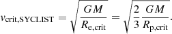
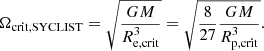
Here Re, crit and Rp, crit are the equatorial radius and the polar radius of a critically rotating star, respectively. The factor 2/3 comes from the relation Re, crit = 3/2Rp, crit in a critically rotating star, in the framework of the Roche approximation. Critical velocity can also be expressed in terms of angular velocity, which in the SYCLIST models is
In general, the variation of the polar radius due to rotation is marginal, such that Rp, crit/RP ≃ 1 is a good approximation, where RP is the polar radius of a star rotating at an arbitrary rate. Therefore, it is possible to calculate Ωcrit, SYCLIST and vcrit, SYCLIST without having a numerical model of a critically rotating star. This definition takes into account the fact that a star will increase its radius as it approaches critical rotation.
However, the MESA stellar models, including our newly computed models and the MESA Isochrones & Stellar Tracks (MIST) models2, adopt a different definition, in which the current equatorial radius Re is used. The critical linear and angular velocities are then defined as:
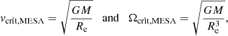
respectively, which are denoted by vorb and Ωorb in Rivinius et al. (2013). This definition indicates the orbital velocity at the equator of a rotating star. As has been stated in Rivinius et al. (2013), a star rotates critically when its equatorial velocity equals the orbital velocity at its equator. In the case of a critically rotating star, vcrit, SYCLIST = vcrit, MESA due to the increase of its equatorial radius. But for noncritically rotating stars, the MESA definition is more meaningful when studying fast-rotating stars with disks, because vcrit, MESA describes which velocity is required for a rotating star to eject material.
The critical velocity fraction is more frequently used than the absolute value of rotational velocity when describing how quickly a star rotates. Under the SYCLIST definition, the critical linear velocity fraction does not equal the critical angular velocity fraction. The relation between them is given by:
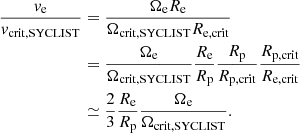
Here ve and Ωe are the equatorial linear and angular velocities, respectively. Under the MESA definition, the fractional linear and angular velocities are identical, that is ve/vcrit, MESA = Ωe/Ωcrit, MESA. Except for the extreme cases of zero rotation and critical rotation, we have ve/vcrit, MESA < ve/vcrit, SYCLIST < Ωe/Ωcrit, SYCLIST.
In this work, we always mean the MESA definition when referring to critical rotation, that is vcrit = vcrit, MESA, because we mainly use our MESA models to investigate the role of rotation in splitting the cluster MS. But in order to compare our models with the SYCLIST models, we use Eq. (11) in Rivinius et al. (2013) to convert the critical velocity fraction of the SYCLIST models to the value under the MESA definition.
It is worth noting that the SYCLIST stellar models undergo a relaxation phase at the very beginning of their MS evolution, lasting for a few percent of their MS lifetimes, during which their rotational velocities decrease dramatically as meridional circulation transports angular momentum from their outer layers to their inner layers (Ekström et al. 2008). The decrease of the surface rotational velocity is more substantial in models with higher initial velocities. In particular, the SYCLIST model formally labeled as ωlabel = Ωe/Ωcrit, SYCLIST = 0.9 has Ωe/Ωcrit, SYCLIST ∼ 0.8 after such relaxation phase, which corresponds to ve/vcrit, MESA ∼ 0.5. Therefore, we stress that the SYCLIST models that are formally labeled as extreme rotation are in fact not rotating that fast.
3. Input physics and assumptions in stellar models
We use the single stellar models described in detail in Wang et al. (2022), which are extended from the models in Schootemeijer et al. (2019). The models are computed by the detailed one-dimensional stellar evolution code MESA, version 12115, (Paxton et al. 2011, 2013, 2015; Paxton et al. 2019). The models include differential rotation, rotationally induced internal mixing and magnetic angular momentum transport. In this section, we briefly summarize the most relevant assumptions in the following and compare them with those used in SYCLIST and MIST models.
The stellar structure of a rapidly rotating star deviates from spherical symmetry due to the presence of the centrifugal force. In a one-dimensional stellar evolution code, stellar structure equations are solved on the isobaric shells that are assumed to have constant angular velocities (Meynet & Maeder 1997). In the MESA code, two factors fT and fP, are introduced to correct temperature and pressure of a rotating star, such that the regular form of the equations of nonrotating stars is retained (Endal & Sofia 1976; Paxton et al. 2013). In the older versions of the MESA code, fT and fP are limited to specific values to ensure numerical stability, which limits the accuracy of computing the stellar models rotating at more than 60% of their critical velocities. However, in version 12115, which is the one we use, a new implementation of the centrifugal effects allows for a precise calculation of the stellar models rotating up to 90% of their critical velocities (Paxton et al. 2019).
We use the standard mixing-length theory to model convection with a mixing length parameter of α = l/HP = 1.5, where HP is the local pressure scale height. The boundary of the convective core is determined by the Ledoux criterion. We adopt step overshooting that extends the convective zone by αOVHP, where αOV varies with mass (see Hastings et al. 2021; Wang et al. 2022 for detail). In the SYCLIST modes, the same method is used with a fixed αOV of 0.1. In the MIST models, an exponentially decaying diffusion coefficient is applied, which is roughly equivalent to αOV = 0.2 in the context of step overshooting. A larger convective overshooting parameter will result in a larger convective core and thus a longer MS lifetime. We adopt a semiconvection mixing efficiency parameter of αSC = 10 (Schootemeijer et al. 2019), and a thermohaline mixing efficiency of αth = 1 (Cantiello & Langer 2010).
Rotationally enhanced mixing is modeled as a diffusive process (Heger et al. 2000), with fc scaling the efficiency of composition mixing with respect to angular momentum transport, and fμ describing the stabilizing effect of mean molecular weight gradients. We adopt values of fc = 1/30 (Chaboyer & Zahn 1992; Marchant et al. 2016) and fμ = 0.1 (Yoon et al. 2006), while the MIST models use the same fc, but a different fμ of 0.05. A smaller fμ value means a more efficient rotational mixing even in the presence of a stabilizing chemical composition gradient. The effects of the dynamical and secular shear instabilities, the Goldreich–Schubert–Fricke instability, and the Eddington-Sweet circulations are included. In the SYCLIST models, a more efficient diffusive-advective approach is taken when modeling rotational mixing, which makes their fast rotators hotter and mroe luminous than our models and than the MIST models with the same initial parameters. We implement the Tayler–Spruit dynamo (Spruit 2002) to transport angular momentum in our MESA models, which imposes a strong coupling between the contracting core and the expanding envelope during stars’ MS evolution. As a consequence, our MESA models rotate nearly as solid bodies. This process is not considered in the SYCLIST models, and consequently, the SYCLIST models rotate differentially and spin down more quickly at the stellar surface than the MESA models (Choi et al. 2016; Hastings et al. 2020). Differential rotation in the SYCLIST models induces shear mixing within the adjacent layers, which also leads to efficient rotational mixing. Despite the difference of these parameters, they are all able to explain some observations but struggle with others (see Choi et al. 2016, for example), meaning that current observations cannot uniquely constrain the uncertain physics in stellar models.
We compute single-star models with both LMC-like metallicity ZLMC = 0.004841 and SMC-like metallicity ZSMC = 0.002179 according to Brott et al. (2011). Our single-star models have initial masses between 1.05 and 19.95 M⊙, which securely covers the magnitude range of MS stars in the LMC cluster NGC 1818, with intervals of log M/M⊙ = 0.04. For each mass, we have nine evolutionary tracks with initial rotational velocities Wi = ve/vcrit, MESA ranging from 0 to 0.8, in intervals of 0.1. Our models start from the zero-age MS (ZAMS) and end when their central helium is depleted.
We notice that our MESA models do not achieve thermal equilibrium initially, which causes wobbles in the stellar radius, and in turn affects their critical and rotational velocities. Unlike in the SYCLIST models, the change of the rotational velocity during this relaxation period is marginal in our MESA models, due to the implementation of a strong core-envelope coupling. To eliminate this uncertain phase, we redefine the ZAMS state as the time when 3% of hydrogen is burnt in the core. We use the rotational velocity ve/vcrit,MESA at that time as the initial velocity Wi. Then we perform interpolation to obtain stellar models with specified Wi values from 0 to 0.75, in intervals of 0.05. To construct isochrones from our stellar models, we use the method described in Wang et al. (2020) to obtain the stellar properties at certain ages. We convert stellar luminosity and temperature to magnitude in the HST/WFC3 F814W filter and a color. For the color we use the difference between the magnitudes in the HST/WFC3 F336W and F814W filters, using the method described in Wang et al. (2022).
To compare our models with the SYCLIST models, we first obtain the appropriate SYCLIST evolutionary tracks and isochrones, with marked ωlabel from 0.0 to 0.95, from their website. We then redefine the SYCLIST models’ ZAMS phase and their initial rotational velocities using the method in Sect. 2. We also interpolate the SYCLIST models to obtain the models rotating at precisely the required values. For the MIST models, only the models with Wi = 0.0 and Wi = 0.4 are available to the public, thus we do not do any redefinition and interpolation to them. This does not affect our comparison, because the MIST models have the same definition of critical velocity as our MESA models, and meanwhile the effect of their initial relaxation phase before 3% H consumption is negligible. We need to point out that in the SYCLIST models, metallicities ZLMC, SYCLIST = 0.006 and ZSMC, SYCLIST = 0.002 are tailored for LMC and SMC stars. The MIST models have multiple metallicities available. We chose two values that are closest to the adopted values in our MESA models, which are ZLMC, MIST = 0.0452 and ZSMC, MIST = 0.00254 for the LMC and SMC stars, respectively. We also need to stress that, apart from the different metallicities, the abundance ratio of the heavy elements are also different in the SYCLIST models and our MESA models. The SYCLIST models simply use solar-scaled abundance ratios, while our models follow the initial chemical compositions in Brott et al. (2011) that are intended to match the observations of the OB stars in the LMC and SMC in the VLT-FLAMES survey (Evans et al. 2005).
4. Results and discussions
4.1. Rotationally induced color variation
We have mentioned in Sect. 1 that the effects of rotation can change stellar effective temperature, luminosity, and lifetime. Previous studies usually inferred the spins for the red and blue MS stars by comparing the photometric observations with the isochrones of stellar models with different rotation (Milone et al. 2018; Gossage et al. 2019; Wang et al. 2022). However, isochrone fitting is a nontrivial task due to many free parameters, including age, initial rotation, distance modulus, and reddening. There is a more straightforward way to infer the spins of the red and blue MS stars in the first place, that is to calculate the color difference of the stellar models with different initial rotational velocities and then compare it with the observed color split of the red and blue MSs in young star clusters. This experiment is not as sensitive to the adopted age, distance modulus, and reddening as isochrone fitting. After acquiring rotational velocities for the red and blue MS stars through this method, we inspect our results by performing isochrone fits to cluster stars in the CMD.
To obtain the observed color split of the red and blue MSs in young star clusters, we utilize previous analyses on the fraction of stars in each MS in three clusters, namely NGC 1755 (see Fig. 5 in Milone et al. 2016), NGC 2164 (see Fig. 13 in Milone et al. 2018) and NGC 1866 (see Fig. 6 in Milone et al. 2017). In these studies, the stellar density distribution as a function of color (mF336W − mF814W) has been scrutinized. We treat the color that has the highest density of the red and blue MS stars as the color of the corresponding population, and then calculate their color difference. We use the magnitude intervals given in these studies. We only take into account the unevolved and less-evolved observed stars, because the split MS feature is prominent among these stars. Meanwhile, focusing on the unevolved and less-evolved stars, which have not been affected by stellar evolution processes, allows us to identify the impact of stellar rotation. The results are shown by the dots with error bars in the last three panels of Fig. 1, with different panels corresponding to different clusters. We convert the apparent magnitude of the observed stars to the absolute magnitude using the distance moduli and reddening values provided in Milone et al. (2018).
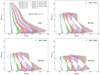 |
Fig. 1. Color difference between the rotating and nonrotating MS stellar models with an LMC metallicity as a function of absolute magnitude MF814W, 0 at four different ages, which are the zero-age and the derived ages for three young LMC clusters NGC 1755 (80 Myr), NGC 2164 (100 Myr) and NGC 1866 (200 Myr) (Milone et al. 2018). The solid, dashed, and dotted lines denote our MESA models, the SYCLIST models and the MIST models, respectively, color-coded by their initial rotational rates. The formally labeled fractional critical angular velocities of the SYCLIST models in their web interface are shown in parentheses. Shaded areas show the Δcolor range occupied by stars with orientations that are between pole-on and equator-on. The dots with error bars in the last three panels indicate the color difference between the red and blue MSs of the abovementioned three clusters (see Fig. 5 in Milone et al. 2016 for NGC 1755, Fig. 13 in Milone et al. 2018 for NGC 2164 and Fig. 6 in Milone et al. 2017 for NGC 1866, respectively). We only consider the unevolved stars below the cluster turnoff (see text). The error bars on the x-axis mean photometric errors while the error bars on the y-axis correspond to magnitude intervals. |
As to the stellar models, we calculate the color separation, Δ color = Δ(mF336W−mF814W), of the isochrones of rotating single-star models and the isochrones of nonrotating single-star models in the color–magnitude diagram at four evolutionary times, that is zero age and the derived ages for the abovementioned three observed clusters. We include our MESA models, the SYCLIST models and the MIST models. The results are shown in Fig. 1.
For our MESA models, we also examine the effect of the inclination of rotation axis on the color of the stellar models with Eqs. (44) and (45) in Paxton et al. (2019). The results are shown by the shaded areas in Fig. 1, with the left and right borderline denoting the pole-on and the equator-on case, respectively. As anticipated, at zero age, the projection effect of gravity darkening is more significant in more rapidly rotating stars. However, the projection effect of gravity darkening also contributes more at high magnitudes. We stress that it is merely a geometric consequence, since the isochrones of the stellar models with different initial rotational velocities have larger horizontal color differences at higher magnitudes (see the red shaded area in the right panel of Fig. 2). At older ages, the effect of gravity darkening becomes significant near the turn-off region. The reason is that gravity darkening either makes a star hotter and brighter (pole-on), or cooler and dimmer (equator-on); therefore, its net effect shifts a star in the CMD almost along the isochrone. Hence, the net effect of gravity darkening is only visible when an isochrone bends toward the right and becomes almost vertical in the turn-off region (also see the red shaded area in the right panel of Fig. 2).
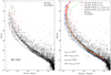 |
Fig. 2. Isochrone fitting to the main-sequence stars in the LMC cluster NGC,1818. Left: distribution of the main-sequence stars in NGC 1818 observed by HST. The black and red dots are normal MS stars and the stars with a brightness excess in the Hα narrow band filter, respectively. The gray error bars on the left indicate 1σ photometric uncertainties at corresponding magnitudes. Right: isochrone fitting to the red and blue MSs of NGC 1818, using the SYCLIST models and our MESA models. For the SYCLIST models, we take the fit in Milone et al. (2018), using 40 Myr isochrones of the nonrotating models and the models with labeled 90% of critical angular velocities (roughly equal to 50% of critical linear velocities under the MESA definition) to fit the observed blue and red MSs, indicated by the solid orange and the dashed green lines, respectively. While for our MESA models, we employ 30 Myr isochrones of the nonrotating models and the models with 50% of critical linear velocities to fit the observed blue and red MSs, denoted by the solid red and the dashed blue lines, respectively. The adopted distance modulus and reddening in each fit are listed. The red shaded area depicts the projection effect (gravity darkening) on the red solid line. The small gray arrow shows how an isochrone would move if E(B − V)=0.05 is added. |
Figure 1 yields three conclusions. Firstly, for the unevolved and less-evolved stellar models in which rotation only plays a role through the centrifugal force, the same initial velocity differences lead to nearly the same color variations in all the three model sets. Secondly, after the ZAMS, the color difference between the rotating and nonrotating models is different in different model sets. Among the three model sets, the SYCLIST models adopt the strongest rotational mixing efficiency (see Sect. 3 and Appendix A). It can be seen that the Δcolor values of the SYCLIST models become smaller than that of our MESA models and the MIST models near the turnoff. In some cases, Δcolor is even negative, meaning that the corresponding SYCLIST rotating models are bluer than their nonrotating models. The adopted rotational mixing efficiency in the MIST models is slightly larger than that in our MESA models (see Sect. 3 and Appendix A). As a consequence, the Δcolor values of the MIST models are between those of the SYCLIST models and our MESA models near the cluster turnoff. The last conclusion is that the color difference between the models with ∼50% of critical rotation, rather than the previously proposed near-critical rotation (D’Antona et al. 2017; Milone et al. 2018), and the models with zero rotation is adequate to retrieve the color split of the observed red and blue MSs in young star clusters. This is consistent with the previous results based on the MESA models (Gossage et al. 2019; Wang et al. 2022). From the star formation point of view, half of the critical rotational velocity agrees with the results of hydrodynamic simulations that take into account the gravitational torques between stars and disks (Lin et al. 2011). We remind the reader that 50% of the critical rotational velocity under the MESA definition roughly equals 60% of critical linear velocity and 75% of critical angular velocity under the definition in the SYCLIST models.
We notice that other combinations of initial rotational velocities are also able to explain the color difference of the observed red and blue MS stars. In Appendix B, we show that Wi ∼ 0.55 and Wi ∼ 0.6 are required to explain the red MS stars, if the blue MS stars have Wi = 0.2 and Wi = 0.3, respectively. Meanwhile, Wang et al. (2022) showed that Wi ∼ 0.65 and Wi ∼ 0.35 can also explain the red and blue MSs in young star clusters. We do not consider even faster rotation for the blue MS stars, otherwise it contradicts the spectroscopically measured low velocity of the blue MS stars in NGC 1818 (see Sect. 4.4).
4.2. Isochrone fitting of the double main sequences in NGC 1818
In the following, we perform isochrone fitting to the red and blue MSs in the LMC cluster NGC 1818 using our findings in Sect. 4.1 that these double MSs can be explained by the stellar models with ∼50% and ∼0% of their initial critical rotational velocities. The left panel of Fig. 2 displays the distribution of the stars with (red dots) and without (black dots) Hα excess in the MS region of NGC 1818. We analyze this cluster because it exhibits a clear double MS feature, and has spectroscopic measurements for the rotational velocity of the stars in different MSs. In the right panel of this figure, we show isochrone fitting based on both our MESA models and the SYCLIST models. We first replicate the isochrone fitting shown in Milone et al. (2018), in which 40 Myr isochrones of the SYCLIST models with ωlabel = 0.9 and ωlabel = 0.0 are used. The adopted distance modulus and reddening are listed both in the figure and in Table 1. As we have mentioned, ωlabel = 0.9 in the SYCLIST models roughly correspond to Wi = 0.5 under the MESA definition.
Models and parameters used in isochrone fittings to NGC 1818.
As to our MESA models, we adapt the isochrone age, distance modulus and reddening, such that the isochrone of our Wi = 0.5 MESA models (solid red line) fits the observed red MS as well as the SYCLIST isochrone, in a visual inspection. We find that a younger age is required when using our MESA models to achieve a satisfactory fit compared to using the SYCLIST models. This is because extensive rotational mixing makes fast-rotating SYCLIST models appear younger, indicating again that different physics assumptions in stellar models can give rise to different results in cluster age estimation. In this figure, we also display the impact of gravity darkening and inclination on our MESA isochrone of the fast-rotating-star models in the CMD. As explained in Sect. 4.1, the influence of gravity darkening in the CMD is only visible in the cluster turn-off area.
We notice that the adopted distance modulus μ = 18.28 for our MESA models is smaller than the measured value for the LMC (μ = 18.49 ± 0.06) (Pietrzyński et al. 2013; Inno et al. 2016). Distance moduli of 18.49 and 18.28 correspond to distances of 49.9 kpc and 45.3 kpc. The diameter of the LMC estimated in Gaia Collaboration (2018) is around 5.2 kpc, meaning that the spatial extent of the LMC clusters is inconsistent with the small value of the adopted distance modulus. We stress here that the adopted distance modulus is sensitive to metallicity and chemical composition of the employed stellar models. Meanwhile, the adopted bolometric correction table also affects the derived distance modulus. Moreover, compared to the distance modulus, the position of an isochrone in the CMD depends more on the adopted reddening. The mean measured reddening of the LMC is E(B − V)=0.113 ± 0.060 mag (Joshi & Panchal 2019). The gray arrow in the right panel of Fig. 2 demonstrates in which direction the isochrones will move in the CMD if reddening is increased by 0.05. In summary, we state that our adopted distance modulus and reddening are in the acceptable range.
Figure 2 supports our previous result that, in both our MESA models and the SYCLIST models, 50% and 0% of critical rotation can explain the best discernible part of the observed red and blue MSs below the cluster turnoff. Our MESA models and the SYCLIST models show different behavior in the turn-off area. The isochrone of the fast-rotating SYCLIST models crosses with that of the slowly-rotating stellar models, as a consequence of strong rotational mixing. In contrast, the isochrone of our fast-rotating MESA models is always redder than the isochrone of our slowly-rotating-star models. It seems that our MESA isochrones match the spread distribution of the turn-off stars better, as the SYCLIST isochrones miss the observed blue MS stars between 16 and 17.5th magnitude in the F814W filter. However, considering the fact that the cluster turn-off area may contain a mixture of stars, including single stars, pre- and post-interaction binaries, we cannot assess these two model sets based on current photometric observations. A plausible way to constrain rotational mixing is to measure the chemical abundance of the H-burning products at the stellar surface. We explore the surface He and N enrichment of our MESA models and the SYCLIST models in Sect. 4.3.
We show in Appendix B that other combinations of rotational velocities can produce equally satisfying isochrone fittings as Fig. 2. This again means that the precise rotational velocity of the cluster stars cannot be solely determined by photometric observations. Nevertheless, the conclusion that moderate and slow rotation is required to explain the split MSs in young star clusters is rigid.
The stars redder than the isochrones of the fast-rotating-star models can be understood by the unresolved binaries containing two fast-rotating components. The presence of a secondary star shifts an observed star to a redder and brighter position in the CMD. The Hα emitters, which are widely considered to rotate at or close to their critical rotational velocities, occupy the reddest part of the CMD, extending ∼2 mag from the cluster turnoff. We discuss the formation of these stars in Sect. 4.5. At last, the stars bluer than the isochrones of the slowly-rotating-star models in Fig. 2 are explained as MS merger products (Wang et al. 2020, 2022). In addition to their slow rotation, MS merger products appear bluer also because of rejuvenation.
4.3. Surface chemical composition
Massive stars burn H through the CNO cycle, in which the rate of the reaction between 14N and 1H is the slowest. This leads to nitrogen enhancement in the layers where nuclear burning takes (or has taken) place. Rotational mixing may take these layers that are enriched in 14N, as well as the H burning ashes He, to the stellar surface. Hence, surface chemical composition abundance can be used as a probe of the strength of rotational mixing. In Fig. 2, we show that our MESA isochrones and the SYCLIST isochrones can fit the split MS in young star clusters equally well, regardless of the different adopted rotational mixing efficiencies. In this section we seek clues to assess these two model sets – or, being more precise, to constrain the strength of rotational mixing – by studying the surface abundance of nitrogen and helium in different stellar models.
Figure 3 shows the surface He and N abundances of the stellar models that are employed in building the isochrones in the right panel of Fig. 2. It can be seen that the rotationally induced surface N enhancement of our MESA models and the SYCLIST models is almost the same (∼10%) at the cluster turnoff. However, a significant enhancement of surface He abundance is only seen in the SYCLIST fast-rotating models. The different behavior of the surface He and N enrichment may be due to the fact that He is produced more slowly than N. When He is produced, a strong chemical composition gradient is created on top of the convective core, which suppresses further mixing of He to the stellar surface in our MESA models, but plays a less important role in the SYCLIST models. The significant surface He enhancement in the SYCLIST fast-rotating models near the cluster turnoff explains their higher temperature. Despite a scarcity of detailed measurements of He abundance of the stars in young star clusters, Carini et al. (2020) found similar surface He abundances for the red and blue MS stars in the turn-off area of the young SMC star cluster NGC 330, which may argue against efficient rotational mixing. Nevertheless, their results should be taken with a grain of salt, given their low S/N, resolution and small sample size. Further observations on more stars in more star clusters are in high demand for our understanding of rotational mixing. We note that recent asteroseismology studies inferred near-rigid rotation in late-B and AF stars (Aerts 2021), and a small amount of differential rotation in massive stars (Bowman 2020), which seems to support our MESA models with efficient angular momentum transfer in the stellar interior.
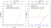 |
Fig. 3. Current surface He (left) and N (right) abundances as a function of magnitude for our MESA models and the SYCLIST models that are used to build the isochrones in Fig. 2. The upper two x-axes show the corresponding mass derived from our MESA models and the SYCLIST models with rapid rotation. |
We have shown that stellar models with Wi = 0.5 exhibit a remarkable surface N enrichment at the end of their MS evolution, in both model sets. In the following, we examine whether the stellar models with other initial velocities also have a surface N enrichment at their TAMS. The results are shown in Fig. 4, with the left and the right panel corresponding to our MESA TAMS models appropriate for the LMC and SMC metallicities, respectively. It can be seen that the stellar models with higher initial velocities and larger initial masses will have larger surface N abundances at their TAMS, which agrees well with the findings in Hastings et al. (2020). Our results indicate that single stars born with spins larger than 40% of their critical values will exhibit a significant N enrichment at the end of their MS evolution.
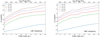 |
Fig. 4. Surface N abundances for our MESA models with the LMC metallicity (left) and the SMC metallicity (right) at the end of their main sequences when 1% of H is left in the stellar center. The x-axis shows the initial mass of the stellar models, with the corresponding cluster turn-off ages shown on the top x-axis. Solid lines with different colors indicate different initial rotational rates. |
4.4. Comparison with the spectroscopic measurements of the rotational velocity of the stars in NGC 1818
By studying photometric observations, we have drawn the conclusion that the red and blue MSs in young star clusters are comprised of the stars with natal spins of 50%–65% and 0%–35% of the critical velocities, respectively. Recently, several high-resolution spectroscopic studies have been performed in young and intermediate-age clusters, providing an unprecedented opportunity to directly measure the rotational rate of the red and the blue MS stars (Dupree et al. 2017; Kamann et al. 2018, 2020; Bastian et al. 2018; Marino et al. 2018; Bodensteiner et al. 2021). Among them, NGC 1818, the cluster we study in this work, is so far, the youngest cluster that has detailed velocity measurements for the stars in different MSs (Marino et al. 2018).
The left panel of Fig. 5 is a zoomed-in version of the CMD of the NGC 1818 MS stars which have magnitudes between 17 and 19. We mark the MS stars whose velocities have been measured spectroscopically in Marino et al. (2018). In the lower right panel, we display the observed v sini of these MS stars as a function of magnitude, and compare them with the stellar models. The average measured velocities for the red and the blue MS stars are 202 ± 23 km s−1 and 71 ± 10 km s−1, respectively, with the red MS stars having a more dispersed velocity distribution. This provides compelling evidence that rotation is responsible for the split MS, with the red MS stars rotating faster than the blue MS stars. The large velocity dispersion of the red MS stars may be attributed to their large intrinsic velocities in combination with the effect of inclination. It is worth noting that all the three red MS stars fainter than ∼18.5th mag are reported to be slow rotators. Marino et al. (2018) argued that the accuracy of the velocity measurement for these faint stars may be affected by their large systematic errors. The Be stars are shown to have the largest v sini values on average. In the upper right panel of this figure, the solid steps show the sum of the number of the observed MS stars in different velocity bins in each population.
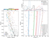 |
Fig. 5. Comparison between the predicted and the observed rotational velocities. Left: a zoom-in image of the main-sequence stars in NGC 1818 which have magnitudes between 17 and 19. The black and red dots correspond to the normal main-sequence stars and Hα emitters, respectively. The open symbols mark the stars that have spectroscopic rotational velocity measurements (Marino et al. 2018), with color indicating their measured projected rotational velocity vsin i values. Here i is the inclination. The red main-sequence stars, blue main-sequence stars, and Be stars with Hα emission lines are designated by triangles, squares and asterisks, respectively. Lower right: comparison between the model predicted average surface equatorial velocity and the spectroscopic measurements. The open symbols with error bars correspond to the observations, using the same symbol types as the left panel. The solid lines and dashed lines represent the average surface equatorial velocity (times π/4 to account for a random orientation) of our MESA models at 30 Myr and the SYCLIST models at 40 Myr (the ages used in our isochrone fitting). Color coding is the same as in Fig. 1. Upper right: comparison between our theoretical predicted vsini distributions (color dotted steps) and the observed vsini distributions of the red (solid black steps) and the blue (solid gray steps) main-sequence stars. For the theoretical predictions, we perform a Monte Carlo simulation by assuming a random orientation angle distribution and normalize the results to a total number of 15 for each initial rotation, which is similar to the number of the blue (14) and red main-sequence (16) stars that have spectroscopic observations. |
To compare with the observations, we display the velocities of our MESA models and the SYCLIST models in the right panels of Fig. 5. In the lower right panel, the red lines demonstrate the average surface rotational velocity (times π/4 to account for a random orientation) of the Wi = 0.5 stellar models along the isochrones that are used to fit the red MS in the right panel of Fig. 2, as a function of magnitude. Then we also display the results for the stellar models that have the same ages but different initial velocities (see other color lines). Consistent with our findings from photometric observations, the current surface velocity of the stellar models with Wi ∼ 0.5 agrees well with the mean observed rotational velocity of the red MS stars (202 ± 23 km s−1). But the three fastest rotating red MS stars can only be explained by the stellar models with initial velocities larger than ∼70% of their critical values, assuming sini = π/4. As to the blue MS stars, the spectroscopic observations report slow, yet clearly non-zero velocities (∼10 − 35% of their critical velocities). In the upper right panel of Fig. 5, we show the number distribution of our MESA models as a function of their velocities with dashed steps. To do this, we again assume a random orientation for our models. We employ our MESA models with Wi = 0.2, 0.5 and 0.6 and consider a Salpeter IMF with the exponent of −2.35 (Salpeter 1955). We generate 106 stellar models and then normalize them to a total number of 15 for each rotational velocity. This number is chosen such that it is similar to the number of the spectroscopically studied red (16) and blue (14) MS stars. Comparing with the observations, we conclude that current velocity of our stellar models with Wi ∼ 0.5 − 0.6 and the stellar models with Wi ∼ 0.2 cover the velocity range of the observed red and blue MS stars well, respectively. The mismatch between the peak of the star model distribution and the observation may be attributed to the small sample size of this observation. Hence, further spectroscopic observations of more stars in this cluster and the stars in other clusters are in high demand to thoroughly constrain the rotation of the cluster MS stars.
4.5. Implications for the origin of Be stars
Currently, two plausible ways have been proposed for the formation of Be stars. The first one is the so-called single-star channel, in which a rotating single star achieves near-critical rotation toward the end of its MS evolution, due to angular momentum transport from the contracting core to the expanding envelope (Ekström et al. 2008; Hastings et al. 2020). The second way is the so-called binary channel, in which the accretor in a binary system spins up during Roche-lobe overflow (Pols et al. 1991; Langer 2012; Wang et al. 2020). The detection of Be/X-ray binaries comprised of a Be star and a compact object (Raguzova & Popov 2005; Liu et al. 2006) and Be+sdO binaries (Peters et al. 2008; Wang et al. 2017; Schootemeijer et al. 2018; Wang et al. 2021) provide direct evidence for the binary channel. However, which fraction of the Be stars has a binary origin is still unknown (Pols et al. 1991; van Bever & Vanbeveren 1997; Shao & Li 2014). Meanwhile, Bodensteiner et al. (2020) found a lack of MS companions to Be stars, which indicates that the binary channel could dominate Be star formation. The Hα emitters detected in young star clusters may deliver new insights into the origin of Be stars. Hastings et al. (2020) stated that the detection of Be stars several magnitudes fainter than the cluster turnoff may advocate the major role of binary interaction in producing Be stars, because the single-star channel can only lead to the Be stars near the cluster turnoff, unless stars are born with extremely high spins. Because they adopted an initial rotational velocity distribution based on the observations of early B stars in the LMC (Dufton et al. 2013) and they used different stellar models (Brott et al. 2011) from ours, we find it helpful to reinvestigate the contribution of single-star evolution in producing Be stars in young star clusters with our MESA models, considering our findings that the red MS stars are born with 50–65% of their critical rotational velocities.
In Fig. 6 we show the surface critical rotational velocity fraction v/vcrit of our LMC models whose magnitudes are between 0.1 and 3 mag (in the F814W filter) below the cluster turnoff. We only consider the stellar models which have initial spins higher than 40% of their critical values, because the stellar models rotating more slowly only change their rotational velocities marginally during their MS evolution and cannot give rise to Be stars. We consider star clusters with ages from 10 to 100 Myr, which are covered well by our stellar models. Nevertheless, our conclusion should apply to star clusters as old as those with cluster ages corresponding to a turn-off mass of around 2.5 M⊙, below which magnetic braking may play a vital role in determining stars’ initial rotational velocities.
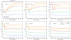 |
Fig. 6. Surface critical velocity fraction v/vcrit of our LMC models with different magnitudes as a function of cluster age. Each panel shows the result for the stellar models with a given magnitude, indicated in the legend. MTO denotes the absolute F814W magnitude of the cluster turnoff. In each panel, different colors correspond to the stellar models with different initial rotational velocities. We show the turn-off mass of the clusters with corresponding ages on the top x-axis in the first panel. |
The last panel of Fig. 6 demonstrates that the stellar models three magnitudes below the cluster turn-off luminosity almost retain their initial rotational velocities. Only the stellar models in clusters younger than ∼30 Myr evolve to slightly higher critical rotational velocity fractions, because the stellar models three magnitudes below the cluster turnoff in such young star clusters are in later evolutionary phases, that is, have consumed more hydrogen, compared to those in older star clusters. The other panels in this figure represent the results for brighter stars. It can be seen that in clusters older than ∼60 Myr, v/vcrit increases with stellar brightness monotonically and even reach close to 1 near the cluster turnoff. While in clusters between 10 and 60 Myr, there is a “U-shape” feature for the stellar models with Wi ≥ 0.6. The right side of the “U-shape” feature is caused by strong stellar winds due to the bi-stability jump, which have a larger impact on more massive stars. While the left side of the “U-shape” feature is a combined effect of a later evolutionary phase of the corresponding stellar models and a smaller impact of the enhanced stellar winds due to the bi-stability jump, because the related massive stellar models are only affected by the bi-stability jump at the very end of their MS evolution. However, whether the bi-stability jump indeed exists and how it affects stellar evolution is still debated (Björklund et al. 2022). We explain this in more detail in Appendix C.
Figure 6 shows that the contribution of single-star evolution to the Be stars in young star clusters depends on how fast single stars initially rotate and how fast B stars have to rotate to become Be stars. Unlike the binary channel that mainly produces near critically rotating Be stars (Wang et al. 2020), the single-star channel gives rise to stars of various rotational velocities. Given the fact that how fast Be stars rotate is disputed (Yudin 2001; Cranmer 2005; Zorec et al. 2016), we only provide some instructive discussions. We have concluded that the red MS stars in young star clusters have 50–65% of their critical rotational velocities. Figure 6 illustrates that the stellar models with Wi = 0.5 cannot give rise to Be stars if we consider 70% of the critical rotational velocity as the threshold for a star to be a Be star, unless in very young star clusters (∼10 Myr). We do not consider an even lower velocity threshold for Be stars, because otherwise the red MS stars may be born as Be stars according to their derived initial spins, which contradicts the observations that Hα emitters are only found within 2–3 mag below the cluster turnoff. If the initial rotational velocity for the red MS stars can be as high as 65% of their critical values, single star evolution is able to explain the Be stars as faint as 2 mag below the cluster turnoff, given a Be star velocity threshold of 70% of critical rotational velocity. But it becomes hard to explain the Be stars with the single-star channel if the Be star velocity threshold is higher than 80% of critical rotation. Near the cluster turn-off region it is stellar winds that prevent stellar models from being Be stars, while below the cluster turn-off stars do not have enough time to evolve to very high spins.
In summary we find that, from the theoretical side, the significance of the role of single-star evolution in producing Be stars in young star clusters depends on the uncertain stellar wind and the uncertain rotational velocity required to form Be stars. Though Wang et al. (2020, 2022) showed that binary evolution can explain the luminosity range of the observed Hα emitters in young star clusters, and Hastings et al. (2021) found that binary interaction alone is able to explain the luminosity range and number fraction of the observed Be stars in young star clusters based on a simple analytical analysis, we cannot exclude the possibility that the single-star channel produces Be stars. Accurate estimation of the spins of Be stars should be useful since, as we have mentioned above, Be stars stemming from the single-star channel should have a larger spin range than those originating from the binary channel. In addition, Be stars originating from the single-star channel usually have a visible surface N enrichment (see Sect. 4.3). On the contrary, the Be stars formed in binary systems may bear a normal N abundance, because the progenitors of these Be stars, that is the accretors, rotate at normal speed until mass transfer starts, at which time a strong chemical composition gradient that can impede a further mixing has been established. But whether binary-evolution-induced Be stars have N enrichment may also depend on the accretion efficiency, as the N enriched layers of the donor stars may remain on the accretors.
We show the results for the SMC models in Fig. C.1. We attain a similar conclusion in the SMC models, but, in general, the SMC models reach higher velocities than their LMC counterparts as a consequence of weaker wind mass loss.
5. Summary and conclusions
There is a growing consensus that a bimodal distribution of rotation rates causes the split MSs in young star clusters. Previous studies proposed that the red and blue MSs are comprised of near-critical rotating stars and nonrotating stars, respectively, by comparing the SYCLIST models with photometric observations. However, the suggestion that most of the stars are born with near-critical rotation contradicts the spectroscopically measured velocity of both cluster and field stars. Gossage et al. (2019) and Wang et al. (2022) argued that the red MS stars should rotate at around half of their critical velocities. In this work, we reinvestigated how much rotation is needed to explain the color split of the observed double MSs in young star clusters, considering our newly computed MESA models, the SYCLIST and the MIST models. We pointed out that it is a misconception that the SYCLIST models formally labeled as rotating at 90% of their critical angular velocities are rotating close to their critical rotational velocity, because of the early relaxation stage of the models and different definitions of critical rotation. We indeed found consistency between our MESA models and the SYCLIST models. Moreover, we found that the cluster MS stars follow a bi-modal velocity distribution, with the majority born with spins of 50–65% of critical rotation constituting the red MS, while a smaller yet significant fraction of stars born with 0–35% of critical rotation constitute the blue MS. This does not only agree with the bimodal velocity distribution found for field B and A type stars (Dufton et al. 2013; Zorec & Royer 2012), but also matches the spectroscopically measured velocities of the red and the blue MS stars in NGC 1818 (Marino et al. 2018).
For our analysis, we found it most useful to focus on the unevolved stars well below the MS turnoff, because near the turnoff, gravity darkening as well as single- and binary-star evolution effects can blur the picture. We show that model sets which use different assumptions about rotational mixing lead to the same results when studying the unevolved stars, but predict different turn-off features. For example, fast-rotating SYCLIST models that adopt efficient rotational mixing are bluer than their slowly-rotating counterparts in the turn-off region. In contrast, in our MESA models and in the MIST models, in which strong rotational mixing is inhibited by chemical composition gradients, fast-rotating models always remain redder than their slowly-rotating counterparts. Current sparse spectroscopic observations find that fast-rotating stars are in general redder than the slowly-rotating ones even near the cluster turnoff, which may support inefficient rotational mixing (Dupree et al. 2017; Marino et al. 2018; Kamann et al. 2020). The surface nitrogen abundance is significantly enhanced in both, MESA and SYCLIST fast-rotating models, but the helium abundance is only enhanced in the fast-rotating SYCLIST models. Spectroscopic measurements of the surface chemical composition of stars in the turn-off region may be able to put tighter constraints on the strength of rotational mixing.
The knowledge of the initial spin distribution of the cluster stars bears important conclusions for their later evolution. Consistent with previous studies, our single-star models increase their critical velocity fraction as a consequence of their contracting core during hydrogen burning. We found that if the rotation-velocity threshold for a star to be a Be star is as low as 70% of the critical velocity, our LMC models starting with 50–65% of their critical velocity can evolve into Be stars before the end of core hydrogen burning. However, for a threshold larger than 80% of critical velocity, it depends on the cluster age whether the initially rapidly rotating single-star models can become Be stars during their MS evolution. A major factor that may prevent stellar models from rotating critically is the strong mass loss due to the bi-stability jump. As discussed above, whether the bi-stability jump exists is disputed. Nevertheless, the uncertain wind mass loss does not affect our finding that in most cases the initially moderately rotating stars (red MS stars) cannot reproduce the Be stars as faint as 2–3 mag below the cluster turnoff. The detection of these faint Be stars in young star clusters implies that binary evolution is an indispensable part of Be star formation, while single-star evolution may still play a role in producing Be stars near the cluster turnoff.
Our conclusion that the vast majority of stars are born with moderately rapid or with slow rotation also affects our understanding of post-MS stars. It implies, that according to our models, rotational mixing may affect the surface abundances of trace elements like boron or nitrogen. But otherwise, rotation is not affecting the evolution of the stars, their post-MS life, supernova type, or the remnant mass in an important way. We might still expect differences in the advanced evolution of blue and red MS stars, perhaps due to different binary properties or different magnetic fields, which would reward study with appropriate stellar models and investigation in future observational campaigns.
Acknowledgments
We thank Dominic Bowman for useful discussions on how asteroseismology constrains the rotational structure of stars. We thank Sebastian Kamann and Nate Bastian for their stimulating discussions. S.d.M. and S.J. acknowledge partial funding by the Netherlands Organization for Scientific Research (NWO) as part of the Vidi research program BinWaves (project number 639.042.728). This work has received funding from the European Research Council (ERC) under the European Union’s Horizon 2020 research innovation programme (Grant Agreement ERC-StG 2016, No 716082 ‘GALFOR’, PI: Milone, http://progetti.dfa.unipd.it/GALFOR), and from MIUR through the FARE project R164RM93XW SEMPLICE (PI: Milone) and the PRIN program 2017Z2HSMF (PI: Bedin).
References
- Aerts, C. 2021, Rev. Mod. Phys., 93, 015001 [Google Scholar]
- Bastian, N., & de Mink, S. E. 2009, MNRAS, 398, L11 [NASA ADS] [CrossRef] [Google Scholar]
- Bastian, N., Cabrera-Ziri, I., Niederhofer, F., et al. 2017, MNRAS, 465, 4795 [NASA ADS] [CrossRef] [Google Scholar]
- Bastian, N., Kamann, S., Cabrera-Ziri, I., et al. 2018, MNRAS, 480, 3739 [NASA ADS] [CrossRef] [Google Scholar]
- Björklund, R., Sundqvist, J. O., Singh, S. M., Puls, J., & Najarro, F. 2022, A&A, accepted [arXiv:2203.08218] [Google Scholar]
- Bodensteiner, J., Shenar, T., & Sana, H. 2020, A&A, 641, A42 [NASA ADS] [CrossRef] [EDP Sciences] [Google Scholar]
- Bodensteiner, J., Sana, H., Wang, C., et al. 2021, A&A, 652, A70 [NASA ADS] [CrossRef] [EDP Sciences] [Google Scholar]
- Bowman, D. M. 2020, Front. Astron. Space Sci., 7, 70 [Google Scholar]
- Brandt, T. D., & Huang, C. X. 2015, ApJ, 807, 25 [NASA ADS] [CrossRef] [Google Scholar]
- Brott, I., de Mink, S. E., Cantiello, M., et al. 2011, A&A, 530, A115 [NASA ADS] [CrossRef] [EDP Sciences] [Google Scholar]
- Cantiello, M., & Langer, N. 2010, A&A, 521, A9 [NASA ADS] [CrossRef] [EDP Sciences] [Google Scholar]
- Carini, R., Biazzo, K., Brocato, E., Pulone, L., & Pasquini, L. 2020, AJ, 159, 152 [NASA ADS] [CrossRef] [Google Scholar]
- Chaboyer, B., & Zahn, J. P. 1992, A&A, 253, 173 [NASA ADS] [Google Scholar]
- Choi, J., Dotter, A., Conroy, C., et al. 2016, ApJ, 823, 102 [Google Scholar]
- Correnti, M., Goudfrooij, P., Bellini, A., Kalirai, J. S., & Puzia, T. H. 2017, MNRAS, 467, 3628 [NASA ADS] [Google Scholar]
- Cranmer, S. R. 2005, ApJ, 634, 585 [NASA ADS] [CrossRef] [Google Scholar]
- D’Antona, F., Di Criscienzo, M., Decressin, T., et al. 2015, MNRAS, 453, 2637 [NASA ADS] [Google Scholar]
- D’Antona, F., Milone, A. P., Tailo, M., et al. 2017, Nat. Astron., 1, 0186 [CrossRef] [Google Scholar]
- de Jager, C., Nieuwenhuijzen, H., & van der Hucht, K. A. 1988, A&AS, 72, 259 [NASA ADS] [Google Scholar]
- Dufton, P. L., Langer, N., Dunstall, P. R., et al. 2013, A&A, 550, A109 [NASA ADS] [CrossRef] [EDP Sciences] [Google Scholar]
- Dupree, A. K., Dotter, A., Johnson, C. I., et al. 2017, ApJ, 846, L1 [NASA ADS] [CrossRef] [Google Scholar]
- Ekström, S., Meynet, G., Maeder, A., & Barblan, F. 2008, A&A, 478, 467 [Google Scholar]
- Ekström, S., Georgy, C., Eggenberger, P., et al. 2012, A&A, 537, A146 [Google Scholar]
- Endal, A. S., & Sofia, S. 1976, ApJ, 210, 184 [NASA ADS] [CrossRef] [Google Scholar]
- Endal, A. S., & Sofia, S. 1978, ApJ, 220, 279 [NASA ADS] [CrossRef] [Google Scholar]
- Evans, C. J., Smartt, S. J., Lee, J. K., et al. 2005, A&A, 437, 467 [NASA ADS] [CrossRef] [EDP Sciences] [Google Scholar]
- Gaia Collaboration (Helmi, A., et al.) 2018, A&A, 616, A12 [NASA ADS] [CrossRef] [EDP Sciences] [Google Scholar]
- Georgy, C., Ekström, S., Granada, A., et al. 2013, A&A, 553, A24 [NASA ADS] [CrossRef] [EDP Sciences] [Google Scholar]
- Girardi, L., Eggenberger, P., & Miglio, A. 2011, MNRAS, 412, L103 [NASA ADS] [Google Scholar]
- Gossage, S., Conroy, C., Dotter, A., et al. 2019, ApJ, 887, 199 [NASA ADS] [CrossRef] [Google Scholar]
- Hastings, B., Wang, C., & Langer, N. 2020, A&A, 633, A165 [NASA ADS] [CrossRef] [EDP Sciences] [Google Scholar]
- Hastings, B., Langer, N., Wang, C., Schootemeijer, A., & Milone, A. P. 2021, A&A, 653, A144 [NASA ADS] [CrossRef] [EDP Sciences] [Google Scholar]
- Heger, A., Langer, N., & Woosley, S. E. 2000, ApJ, 528, 368 [NASA ADS] [CrossRef] [Google Scholar]
- Huang, W., Gies, D. R., & McSwain, M. V. 2010, ApJ, 722, 605 [Google Scholar]
- Inno, L., Bono, G., Matsunaga, N., et al. 2016, ApJ, 832, 176 [Google Scholar]
- Joshi, Y. C., & Panchal, A. 2019, A&A, 628, A51 [NASA ADS] [CrossRef] [EDP Sciences] [Google Scholar]
- Kamann, S., Bastian, N., Husser, T. O., et al. 2018, MNRAS, 480, 1689 [Google Scholar]
- Kamann, S., Bastian, N., Gossage, S., et al. 2020, MNRAS, 492, 2177 [Google Scholar]
- Keller, S. C., & Bessell, M. S. 1998, A&A, 340, 397 [NASA ADS] [Google Scholar]
- Langer, N. 2012, ARA&A, 50, 107 [CrossRef] [Google Scholar]
- Li, C., de Grijs, R., Deng, L., & Milone, A. P. 2017, ApJ, 844, 119 [CrossRef] [Google Scholar]
- Lin, M.-K., Krumholz, M. R., & Kratter, K. M. 2011, MNRAS, 416, 580 [NASA ADS] [Google Scholar]
- Liu, Q. Z., van Paradijs, J., & van den Heuvel, E. P. J. 2006, A&A, 455, 1165 [NASA ADS] [CrossRef] [EDP Sciences] [Google Scholar]
- Maeder, A., & Meynet, G. 2000, ARA&A, 38, 143 [Google Scholar]
- Marchant, P., Langer, N., Podsiadlowski, P., Tauris, T. M., & Moriya, T. J. 2016, A&A, 588, A50 [NASA ADS] [CrossRef] [EDP Sciences] [Google Scholar]
- Marino, A. F., Przybilla, N., Milone, A. P., et al. 2018, AJ, 156, 116 [NASA ADS] [CrossRef] [Google Scholar]
- Meynet, G., & Maeder, A. 1997, A&A, 321, 465 [NASA ADS] [Google Scholar]
- Milone, A. P., Marino, A. F., D’Antona, F., et al. 2016, MNRAS, 458, 4368 [NASA ADS] [CrossRef] [Google Scholar]
- Milone, A. P., Marino, A. F., D’Antona, F., et al. 2017, MNRAS, 465, 4363 [NASA ADS] [CrossRef] [Google Scholar]
- Milone, A. P., Marino, A. F., Di Criscienzo, M., et al. 2018, MNRAS, 477, 2640 [Google Scholar]
- Nieuwenhuijzen, H., & de Jager, C. 1990, A&A, 231, 134 [NASA ADS] [Google Scholar]
- Niederhofer, F., Georgy, C., Bastian, N., & Ekström, S. 2015, MNRAS, 453, 2070 [NASA ADS] [CrossRef] [Google Scholar]
- Paxton, B., Bildsten, L., Dotter, A., et al. 2011, ApJS, 192, 3 [Google Scholar]
- Paxton, B., Cantiello, M., Arras, P., et al. 2013, ApJS, 208, 4 [Google Scholar]
- Paxton, B., Marchant, P., Schwab, J., et al. 2015, ApJS, 220, 15 [Google Scholar]
- Paxton, B., Smolec, R., Schwab, J., et al. 2019, ApJS, 243, 10 [Google Scholar]
- Peters, G. J., Gies, D. R., Grundstrom, E. D., & McSwain, M. V. 2008, ApJ, 686, 1280 [Google Scholar]
- Pietrzyński, G., Graczyk, D., Gieren, W., et al. 2013, Nature, 495, 76 [Google Scholar]
- Pols, O. R., Cote, J., Waters, L. B. F. M., & Heise, J. 1991, A&A, 241, 419 [NASA ADS] [Google Scholar]
- Raguzova, N. V., & Popov, S. B. 2005, Astron. Astrophys. Trans., 24, 151 [Google Scholar]
- Rivinius, T., Carciofi, A. C., & Martayan, C. 2013, A&ARv, 21, 69 [Google Scholar]
- Salpeter, E. E. 1955, ApJ, 121, 161 [Google Scholar]
- Schootemeijer, A., Götberg, Y., de Mink, S. E., Gies, D., & Zapartas, E. 2018, A&A, 615, A30 [NASA ADS] [CrossRef] [EDP Sciences] [Google Scholar]
- Schootemeijer, A., Langer, N., Grin, N. J., & Wang, C. 2019, A&A, 625, A132 [NASA ADS] [CrossRef] [EDP Sciences] [Google Scholar]
- Shao, Y., & Li, X.-D. 2014, ApJ, 796, 37 [Google Scholar]
- Spruit, H. C. 2002, A&A, 381, 923 [CrossRef] [EDP Sciences] [Google Scholar]
- van Bever, J., & Vanbeveren, D. 1997, A&A, 322, 116 [NASA ADS] [Google Scholar]
- Vink, J. S., de Koter, A., & Lamers, H. J. G. L. M. 2001, A&A, 369, 574 [NASA ADS] [CrossRef] [EDP Sciences] [Google Scholar]
- von Zeipel, H. 1924, MNRAS, 84, 665 [NASA ADS] [CrossRef] [Google Scholar]
- Wang, L., Gies, D. R., & Peters, G. J. 2017, ApJ, 843, 60 [Google Scholar]
- Wang, C., Langer, N., Schootemeijer, A., et al. 2020, ApJ, 888, L12 [NASA ADS] [CrossRef] [Google Scholar]
- Wang, L., Gies, D. R., Peters, G. J., et al. 2021, AJ, 161, 248 [Google Scholar]
- Wang, C., Langer, N., Schootemeijer, A., et al. 2022, Nat. Astron., 6, 480 [NASA ADS] [CrossRef] [Google Scholar]
- Yang, W., Bi, S., Meng, X., & Liu, Z. 2013, ApJ, 776, 112 [NASA ADS] [CrossRef] [Google Scholar]
- Yoon, S. C., Langer, N., & Norman, C. 2006, A&A, 460, 199 [NASA ADS] [CrossRef] [EDP Sciences] [Google Scholar]
- Yudin, R. V. 2001, A&A, 368, 912 [NASA ADS] [CrossRef] [EDP Sciences] [Google Scholar]
- Zorec, J., & Royer, F. 2012, A&A, 537, A120 [NASA ADS] [CrossRef] [EDP Sciences] [Google Scholar]
- Zorec, J., Frémat, Y., Domiciano de Souza, A., et al. 2016, A&A, 595, A132 [NASA ADS] [CrossRef] [EDP Sciences] [Google Scholar]
Appendix A: Examples of stellar evolution in the HRD
Figure A.1 displays the evolutionary tracks of 5 M⊙ models with different initial rotational velocities in the HRD. The left and the right panels correspond to the LMC and SMC metallicity, respectively. We take into account our MESA models, the SYCLIST models and the MIST models. We have redefined the initial critical velocity fraction for the SYCLIST models, such that it matches the definition used in our MESA models (see Sec. 3). As a reference, we show the formally labeled critical angular velocity fraction of the SYCLIST models in brackets. As mentioned in Sec. 3, the SYCLIST models use a larger metallicity Z appropriate for the LMC stars than our MESA models and the MIST models. As a consequence, the SYCLIST ZAMS models are cooler than the corresponding MESA models in this work and the MIST models at the same velocities. Whereas all three model sets adopt similar metallicity tailored for the SMC stars, therefore, their ZAMS models occupy similar positions in the HRD.
It can be seen in Fig. A.1 that at the ZAMS, when evolutionary effects have not kicked in, the fast-rotating models are cooler than the slowly-rotating models in all three model sets, with similar rotation difference resulting in similar temperature variation. This means that the implementation of the impact of centrifugal force in the three model sets is consistent. Nevertheless, after the ZAMS, the models in different model sets evolve differently, even for the nonrotating-star models. The discrepancy of the evolutionary tracks of the nonrotating stars is caused by different internal mixing. For a 5 M⊙ star, αOV roughly equals 0.1, 0.15 and 0.2 in terms of step overshooting in the SYCLIST models, our MESA models and the MIST models, respectively. Consequently, the SYCLIST nonrotating-star models have the lowest turn-off luminosities and the shortest MS lifetimes, while the MIST models are opposite.
Whereas the diverse evolution of the rotating-star models in different model sets is mainly due to different rotationally induced mixing efficiencies. In contrast to our MESA models and the MIST models, in which the fast-rotating models are always cooler than their slowly-rotating counterparts, the evolutionary tracks of the SYCLIST fast-rotating-star models cross that of the nonrotating models near the end of the MS evolution. This is because in the SYCLIST models, helium is efficiently mixed into the stellar surface even in the presence of a chemical composition gradient. Figure A.2 compares relative enhancement of the surface He abundance of different stellar models. It can be seen that rotational mixing is the strongest in the SYCLIST models, but modest in the MIST models and negligible in our MESA models. It is worth noting that rotational mixing increases the MS lifetime of the SYCLIST rotating models by an overall amount of ∼ 25% (Ekström et al. 2012), while it only increases the MS lifetime of our MESA and the MIST rotating models modestly.
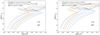 |
Fig. A.1. Evolutionary tracks of 5 M⊙ stellar models with LMC-like (left) and SMC-like (right) metallicities. The solid blue, dashed orange and dotted purple lines denote our MESA models, the SYCLIST models, and the MIST models, respectively. The adopted metallicity Z in different model sets are listed in the legend. In each model set, stellar evolutionary tracks from left to right correspond to models with increasing initial rotational velocity, with values listed in the legend. Numbers in the parentheses indicate the formally labeled fractional critical angular velocities in the SCYLIST web interface. |
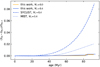 |
Fig. A.2. Surface helium enhancement of 5 M⊙ SMC stellar models as a function of stellar age. The y-axis shows the increase of the surface helium abundance of the stellar models with respect to their initial abundance. Here XHe and XHe, 0 are the current surface helium abundance and the initial surface helium abundance of the stellar models, respectively. The orange solid line corresponds to our nonrotating MESA models, while the solid, dashed, and dotted blue lines correspond to our MESA models, the SYCLIST models, and the MIST models that initially rotate at 40% of their critical velocities. |
Appendix B: Degeneracy in explaining the split main sequence as the effect of rotation
Degeneracy exits in interpreting the observed split MS in young star clusters as the effect of rotation, because different combinations of slow and fast rotation can retrieve the observed color separation between the red and blue MSs equally well. Figures. B.1 and B.2 are similar to Fig. 1, but Δcolor is calculated by using the isochrones of the Wi = 0.20, Wi = 0.30 star modes as the baselines. In these three cases, Wi ∼ 0.55, Wi ∼ 0.60 are required to explain the observed color separation between the red and blue MSs, respectively. Wang et al. (2022) also use Wi ∼ 0.65 and Wi ∼ 0.35 to fit the red and blue MSs in young star clusters.
In Fig. B.3, we perform isochrone fittings to the red and the blue MS stars in NGC 1818, using our MESA models with the abovementioned initial velocities. After adjusting distance modulus and reddening, we attain isochrone fittings that are as good as those shown in the right panel of Fig. 2, which implies that photometric observations are not enough to constrain stars’ precise rotation. Further spectroscopic observations are encouraged.
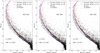 |
Fig. B.3. Same as Fig. 2, but we only show our MESA models and use pairs of isochrones of the Wi = 0.55 and Wi = 0.20 (left), the Wi = 0.60 and Wi = 0.30 (middle), and the Wi = 0.65 and Wi = 0.35 (right) models to fit the observed red and blue main sequences in NGC 1818. |
Appendix C: Surface velocity of the main-sequence models
In this appendix, we continue our discussion in Sec. 4.5 on how will our finding, that the majority of the stars should be born with moderate rotation, change our perception of Be star formation. First of all, we display Fig. C.1, which is similar to Fig. 6, but for the SMC models. In the following, we explain more about this figure and Fig 6 by showing some evolutionary examples of our MESA models and the SYCLIST models. The left panel of Fig. C.2 shows the evolutionary tracks of the selected stellar models in the HRD. The gray shaded area indicates the temperature zone where the stellar mass loss rate in our MESA models is affected by the bi-stability jump. The bi-stability jump temperature is set by eqs. 14 and 15 in Vink et al. (2001). The gray shaded area is a buffer zone with a temperature range of 10% of the bi-stability jump temperature. In this buffer zone, the mass loss rate is computed by interpolating between the winds for hot stars (Vink et al. 2001) and the winds for cool stars (i.e., the maximum value between the mass loss rate computed from Vink et al. (2001) and Nieuwenhuijzen & de Jager (1990)). The right panels of this figure show the mass loss history and the surface velocity evolution of the selected stellar models. We see that our 15 M⊙ LMC model with Wi = 0.7 achieves near critical-rotation at ∼12 Myr and then suddenly spins down to v/vcrit ∼ 0.55, which roughly equals the spin of our LMC model with Wi = 0.4 at the TAMS, due to strong stellar winds. The first peak of the mass loss rate of this star model is caused by critical rotation, while the later steady increase and the plateau between ∼12.5 and 13.75 Myr is due to the bi-stability jump. The bi-stability jump related stellar winds have a larger impact on the stellar models with higher initial velocities. Nevertheless, the 15 M⊙ SMC star model with Wi = 0.7 does not spin down as much as its LMC counterpart because it enters the bi-stability jump temperature zone later and therefore spends less time with the enhanced stellar wind mass loss. A similar feature of a velocity bump before the end of MS evolution is also seen in the 15 M⊙ models in Hastings et al. (2020).
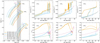 |
Fig. C.2. The left panel shows the evolutionary tracks of the rotating single-star models in different model sets in the Hertzsprung-Russell diagram. The thick orange lines correspond to our MESA models with higher initial rotational velocity, with solid and dashed lines denoting the LMC metallicity and the SMC metallicity, respectively. While the thick blue lines represent our MESA models with lower initial rotational velocity. The thin purple and green lines denote the SYCLIST models that have initial fast and slow spins, respectively. The mass of the stellar models are listed. The gray shaded area indicates the temperature region in which we consider the bi-stability jump related stellar wind for our MESA models. The other three columns of panels illustrate the evolution of mass loss rate and critical velocity (see Eq.3) fraction as a function of stellar age, for three different masses. The meaning of the lines are the same as in the left panel. |
The behavior of the 12 M⊙ models is similar to the 15 M⊙ models, but the TAMS spin of the 12 M⊙ LMC model with Wi = 0.7 is slightly larger than that of the 15 M⊙ counterpart, due to less intense stellar winds. Differently, the 10 M⊙ models reach the bi-stability jump temperature at an early time. The enhanced stellar winds prevent our MESA models from rotating critically, but they are not sufficient to significantly brake the stellar models. Again in this case, the SMC models achieve the bi-stability jump temperature later, and therefore, have higher surface velocities during their MS evolution than their LMC counterparts. Stars less massive than 10 M⊙ start to get rid of the effect of the bi-stability jump and can reach near critical rotation at their TAMS, as their wind mass loss rates are quite low even in the bi-stability jump regime. Figure C.2 helps us understand why the initially fast-rotating-star models in certain mass ranges cannot reach as high velocity as in other mass ranges, which is the feature seen in Fig. 6. In contrast to our MESA models, all the selected SYCLIST models do not experience such a spin down, because they adopt de Jager et al. (1988) winds that do not include the bi-stability jump. We do not attempt to assess the mass loss recipes in different model sets because stellar wind is one of the least constrained physics in astronomy, but we mean to demonstrate that initially moderately rotating single stars are able to reach higher velocities, depending on the competition between angular momentum transport from the stellar center to the stellar surface and angular momentum lost accompanied by stellar winds.
At last, we directly examine the current surface rotational velocity of the stellar models to explore if single star evolution can interpret the observed Be stars in NGC 1818. We have exhibited current velocity of the stellar models in the lower right panel of Fig. 5, but it is in terms of vsini and only for the models ∼1.5 magnitudes fainter than the cluster turnoff. Here we show current critical rotation fraction of the stellar models as a function of their apparent magnitude in Fig C.3. The red solid and dashed lines are the stellar models that are employed in fitting the red MS stars in NGC 1818 (i.e., the stellar models that are used in constructing the red and orange solid lines in the right panel of Fig. 2). The other lines represent the results for the stellar models with other initial velocities, using the same distance moduli and reddenings. In general, v/vcrit increases steadily from high magnitude (unevolved part) to low magnitude (evolved part) until the turn-off magnitude, at which v/vcrit increases dramatically. The turn-over at around 16.5th magnitude for our MESA models with Wi ≥ 0.6 is caused by the spin-down of the turn-off stars caused by the bi-stability jump. Figure C.3 directly shows that the stars ∼1.5 magnitude fainter than the cluster turn-off magnitude almost retain their initial spins. It can be seen that even for the initially rapidly rotating stars (∼60% of critical velocities), single star evolution can only contribute to the Be stars at most 1.5 magnitude below the cluster turnoff, given a Be star velocity threshold of 70% of break-up values. To explain the origin of the fainter Be stars, binary interaction is needed.
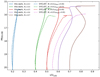 |
Fig. C.3. Current surface rotational rates for our MESA models (solid line) and the SYCLIST models (dashed line). The adopted model age, distance modulus and reddening for each model set are the same as the right panel of Fig. 2. Color coding is the same as Fig. 1. |
All Tables
All Figures
|
Fig. 1. Color difference between the rotating and nonrotating MS stellar models with an LMC metallicity as a function of absolute magnitude MF814W, 0 at four different ages, which are the zero-age and the derived ages for three young LMC clusters NGC 1755 (80 Myr), NGC 2164 (100 Myr) and NGC 1866 (200 Myr) (Milone et al. 2018). The solid, dashed, and dotted lines denote our MESA models, the SYCLIST models and the MIST models, respectively, color-coded by their initial rotational rates. The formally labeled fractional critical angular velocities of the SYCLIST models in their web interface are shown in parentheses. Shaded areas show the Δcolor range occupied by stars with orientations that are between pole-on and equator-on. The dots with error bars in the last three panels indicate the color difference between the red and blue MSs of the abovementioned three clusters (see Fig. 5 in Milone et al. 2016 for NGC 1755, Fig. 13 in Milone et al. 2018 for NGC 2164 and Fig. 6 in Milone et al. 2017 for NGC 1866, respectively). We only consider the unevolved stars below the cluster turnoff (see text). The error bars on the x-axis mean photometric errors while the error bars on the y-axis correspond to magnitude intervals. |
| In the text | |
|
Fig. 2. Isochrone fitting to the main-sequence stars in the LMC cluster NGC,1818. Left: distribution of the main-sequence stars in NGC 1818 observed by HST. The black and red dots are normal MS stars and the stars with a brightness excess in the Hα narrow band filter, respectively. The gray error bars on the left indicate 1σ photometric uncertainties at corresponding magnitudes. Right: isochrone fitting to the red and blue MSs of NGC 1818, using the SYCLIST models and our MESA models. For the SYCLIST models, we take the fit in Milone et al. (2018), using 40 Myr isochrones of the nonrotating models and the models with labeled 90% of critical angular velocities (roughly equal to 50% of critical linear velocities under the MESA definition) to fit the observed blue and red MSs, indicated by the solid orange and the dashed green lines, respectively. While for our MESA models, we employ 30 Myr isochrones of the nonrotating models and the models with 50% of critical linear velocities to fit the observed blue and red MSs, denoted by the solid red and the dashed blue lines, respectively. The adopted distance modulus and reddening in each fit are listed. The red shaded area depicts the projection effect (gravity darkening) on the red solid line. The small gray arrow shows how an isochrone would move if E(B − V)=0.05 is added. |
| In the text | |
|
Fig. 3. Current surface He (left) and N (right) abundances as a function of magnitude for our MESA models and the SYCLIST models that are used to build the isochrones in Fig. 2. The upper two x-axes show the corresponding mass derived from our MESA models and the SYCLIST models with rapid rotation. |
| In the text | |
|
Fig. 4. Surface N abundances for our MESA models with the LMC metallicity (left) and the SMC metallicity (right) at the end of their main sequences when 1% of H is left in the stellar center. The x-axis shows the initial mass of the stellar models, with the corresponding cluster turn-off ages shown on the top x-axis. Solid lines with different colors indicate different initial rotational rates. |
| In the text | |
|
Fig. 5. Comparison between the predicted and the observed rotational velocities. Left: a zoom-in image of the main-sequence stars in NGC 1818 which have magnitudes between 17 and 19. The black and red dots correspond to the normal main-sequence stars and Hα emitters, respectively. The open symbols mark the stars that have spectroscopic rotational velocity measurements (Marino et al. 2018), with color indicating their measured projected rotational velocity vsin i values. Here i is the inclination. The red main-sequence stars, blue main-sequence stars, and Be stars with Hα emission lines are designated by triangles, squares and asterisks, respectively. Lower right: comparison between the model predicted average surface equatorial velocity and the spectroscopic measurements. The open symbols with error bars correspond to the observations, using the same symbol types as the left panel. The solid lines and dashed lines represent the average surface equatorial velocity (times π/4 to account for a random orientation) of our MESA models at 30 Myr and the SYCLIST models at 40 Myr (the ages used in our isochrone fitting). Color coding is the same as in Fig. 1. Upper right: comparison between our theoretical predicted vsini distributions (color dotted steps) and the observed vsini distributions of the red (solid black steps) and the blue (solid gray steps) main-sequence stars. For the theoretical predictions, we perform a Monte Carlo simulation by assuming a random orientation angle distribution and normalize the results to a total number of 15 for each initial rotation, which is similar to the number of the blue (14) and red main-sequence (16) stars that have spectroscopic observations. |
| In the text | |
|
Fig. 6. Surface critical velocity fraction v/vcrit of our LMC models with different magnitudes as a function of cluster age. Each panel shows the result for the stellar models with a given magnitude, indicated in the legend. MTO denotes the absolute F814W magnitude of the cluster turnoff. In each panel, different colors correspond to the stellar models with different initial rotational velocities. We show the turn-off mass of the clusters with corresponding ages on the top x-axis in the first panel. |
| In the text | |
|
Fig. A.1. Evolutionary tracks of 5 M⊙ stellar models with LMC-like (left) and SMC-like (right) metallicities. The solid blue, dashed orange and dotted purple lines denote our MESA models, the SYCLIST models, and the MIST models, respectively. The adopted metallicity Z in different model sets are listed in the legend. In each model set, stellar evolutionary tracks from left to right correspond to models with increasing initial rotational velocity, with values listed in the legend. Numbers in the parentheses indicate the formally labeled fractional critical angular velocities in the SCYLIST web interface. |
| In the text | |
|
Fig. A.2. Surface helium enhancement of 5 M⊙ SMC stellar models as a function of stellar age. The y-axis shows the increase of the surface helium abundance of the stellar models with respect to their initial abundance. Here XHe and XHe, 0 are the current surface helium abundance and the initial surface helium abundance of the stellar models, respectively. The orange solid line corresponds to our nonrotating MESA models, while the solid, dashed, and dotted blue lines correspond to our MESA models, the SYCLIST models, and the MIST models that initially rotate at 40% of their critical velocities. |
| In the text | |
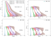 |
Fig. B.1. Same as Fig. 1, but color differences are calculated with respect to the Wi = 0.2 models. |
| In the text | |
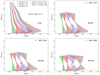 |
Fig. B.2. Same as Fig. 1, but color differences are calculated with respect to the Wi = 0.3 models. |
| In the text | |
|
Fig. B.3. Same as Fig. 2, but we only show our MESA models and use pairs of isochrones of the Wi = 0.55 and Wi = 0.20 (left), the Wi = 0.60 and Wi = 0.30 (middle), and the Wi = 0.65 and Wi = 0.35 (right) models to fit the observed red and blue main sequences in NGC 1818. |
| In the text | |
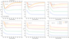 |
Fig. C.1. Similar as Fig. 6, but for the SMC models. |
| In the text | |
|
Fig. C.2. The left panel shows the evolutionary tracks of the rotating single-star models in different model sets in the Hertzsprung-Russell diagram. The thick orange lines correspond to our MESA models with higher initial rotational velocity, with solid and dashed lines denoting the LMC metallicity and the SMC metallicity, respectively. While the thick blue lines represent our MESA models with lower initial rotational velocity. The thin purple and green lines denote the SYCLIST models that have initial fast and slow spins, respectively. The mass of the stellar models are listed. The gray shaded area indicates the temperature region in which we consider the bi-stability jump related stellar wind for our MESA models. The other three columns of panels illustrate the evolution of mass loss rate and critical velocity (see Eq.3) fraction as a function of stellar age, for three different masses. The meaning of the lines are the same as in the left panel. |
| In the text | |
|
Fig. C.3. Current surface rotational rates for our MESA models (solid line) and the SYCLIST models (dashed line). The adopted model age, distance modulus and reddening for each model set are the same as the right panel of Fig. 2. Color coding is the same as Fig. 1. |
| In the text | |
Current usage metrics show cumulative count of Article Views (full-text article views including HTML views, PDF and ePub downloads, according to the available data) and Abstracts Views on Vision4Press platform.
Data correspond to usage on the plateform after 2015. The current usage metrics is available 48-96 hours after online publication and is updated daily on week days.
Initial download of the metrics may take a while.