| Issue |
A&A
Volume 669, January 2023
|
|
|---|---|---|
| Article Number | A61 | |
| Number of page(s) | 15 | |
| Section | Cosmology (including clusters of galaxies) | |
| DOI | https://doi.org/10.1051/0004-6361/202244658 | |
| Published online | 06 January 2023 | |
Forecasts for cosmological measurements based on the angular power spectra of AGN and clusters of galaxies in the SRG/eROSITA all-sky survey
1
Max Planck Institute for Astrophysics, Karl-Schwarzschild-Str 1, Garching b. München 85741, Germany
e-mail: This email address is being protected from spambots. You need JavaScript enabled to view it.
2
Kazan Federal University, Department of Astronomy and Satellite Geodesy, 420008 Kazan, Russia
3
Space Research Institute, Russian Academy of Sciences, Profsoyuznaya 84/32, 117997 Moscow, Russia
Received:
2
August
2022
Accepted:
2
November
2022
Abstract
Context. The eROSITA X-ray telescope aboard the Spectrum-Roentgen-Gamma (SRG) orbital observatory, in the course of its all-sky survey, is expected to detect about three million active galactic nuclei (AGNs) and approximately one hundred thousand clusters and groups of galaxies. Such a sample, clean and uniform, complemented with redshift information, will open a new window into the studies of the large-scale structure (LSS) of the Universe and the determination of its cosmological parameters.
Aims. The purpose of this work is to assess the prospects of cosmological measurements with the eROSITA sample of AGNs and clusters of galaxies. We assumed the availability of photometric redshift measurements for eROSITA sources and explored the impact of their quality on our forecasts.
Methods. As the LSS probe, we use the redshift-resolved angular power spectrum of the density fluctuations of objects. We employed a Fisher-matrix formalism and assumed flat ΛCDM cosmology to forecast the constraining power of eROSITA samples of AGNs and clusters of galaxies. We computed the LSS-relevant characteristics of AGNs and clusters in the framework of the halo model and their X-ray luminosity functions. As the baseline scenario, we considered the full four-year all-sky survey and investigated the impact of reducing the survey length to two years.
Results. We find that the accuracy of photometric redshift estimates has a more profound effect on cosmological measurements than the fraction of catastrophic errors. Under realistic assumptions about the photometric redshift quality, the marginalised errors on the cosmological parameters achieve 1 − 10% accuracy depending on the cosmological priors used from other experiments. The statistical significance of Baryon acoustic oscillation detection in angular power spectra of AGNs and clusters of galaxies considered individually achieves 5 − 6σ. Our results demonstrate that the eROSITA sample of AGNs and clusters of galaxies used in combination with currently available photometric redshift estimates will provide cosmological constraints on a par with dedicated optical LSS surveys.
Key words: X-rays: galaxies / X-rays: galaxies: clusters / large-scale structure of Universe
© The Authors 2023
 Open Access article, published by EDP Sciences, under the terms of the Creative Commons Attribution License (https://creativecommons.org/licenses/by/4.0), which permits unrestricted use, distribution, and reproduction in any medium, provided the original work is properly cited.
This article is published in open access under the Subscribe-to-Open model.
Open Access funding provided by Max Planck Society.
1. Introduction
The distribution of matter in the Universe is not uniform. Galaxies form the so-called cosmic web, comprising filaments, walls, and voids, which make up the large-scale structure (LSS) of the Universe (Dodelson 2003; Eisenstein et al. 2005; Beutler et al. 2011; Alam et al. 2017). Mapping the LSS yields a wealth of important information about cosmological parameters, the evolution of density perturbations, the growth of structures, and the mass-energy content of the Universe (Tegmark et al. 2004; Percival et al. 2010; Blake et al. 2011; Padmanabhan et al. 2012; Abbott et al. 2022a,b). The LSS is traced not only by normal galaxies but also by active galactic nuclei (AGNs) and clusters of galaxies.
The large-scale structure has been probed by several wide-angle optical galaxy surveys such as SDSS (Sloan Digital Sky Survey)1, DES (Dark Energy Survey2), 2dF (2dF Galaxy Redshift Survey3). Using spectroscopic or photometric redshifts of the objects, such surveys unveil the 3D distribution of visible matter in the Universe, permitting us to measure its power spectrum and to detect and quantify various cosmologically significant effects such as baryon acoustic oscillations (BAOs, Sunyaev & Zeldovich 1970; Peebles & Yu 1970) and redshift-space distortions (RSD, Kaiser 1987). These data allow one to measure cosmological parameters (Cole et al. 2005; Eisenstein et al. 2005; Abbott et al. 2022a,b; Alam et al. 2021). Planned space missions and ground-based facilities, such as Euclid4, the Vera Rubin observatory5, the Dark Energy Spectroscopic Instrument6, and the Nancy Grace Roman Telescope7 will dramatically increase the number of objects available for cosmological studies, potentially increasing the accuracy of cosmological measurements.
To date, all cosmologically significant large-scale structure surveys have been conducted in visible light. However, the selection of galaxies and quasars in optical wavelengths is complicated by a number of effects, such as contamination by stars and nearby galaxies, absorption, and several others. On the contrary, X-ray surveys represent an efficient tool for identifying accreting supermassive black holes – indeed, AGNs constitute the majority of sources detected in extragalactic X-ray surveys (e.g., Brandt & Hasinger 2005; Sunyaev et al. 2021). Deep (but relatively narrow, up to ∼25 sq. degrees) X-ray surveys performed by XMM-Newton and Chandra observatories demonstrated the feasibility and usefulness of studying the clustering of X-ray-selected AGNs (Allevato et al. 2011, 2019; Mountrichas et al. 2016; Kolodzig et al. 2017, 2018). Furthermore, hot intracluster medium shines in X-rays by which means one can detect a cluster of galaxies without actually registering individual galaxies. X-ray data allow the determination of cluster mass and temperature, quantities essential for astrophysics and cosmology (e.g., Vikhlinin et al. 2009a,b; Allen et al. 2011). Thus, X-ray-selected samples present a reasonably clean and complete flux-limited census of extragalactic objects – AGNs and clusters of galaxies – for which number density is sufficient to study the LSS.
The SRG orbital X-ray observatory (Sunyaev et al. 2021) was launched into the halo orbit around the Sun-Earth Lagrangian L2 point on July 13, 2019, and on December 12, 2019 an all-sky survey began, which was planned to continue for four years, until December 2023. So far, the eROSITA telescope has completed 4.4 full sky surveys and currently is in safe mode. The SRG observatory continues science observations in the interests of the Mikhail Pavlinsky ART-XC telescope – the second science instrument aboard the SRG observatory.
In the course of the full four-year all-sky survey, the eROSITA telescope (Predehl et al. 2021) aboard SRG is expected to detect, in the 0.5 − 2 keV energy range, ∼3 million AGNs with a median redshift of z ∼ 1 (Kolodzig et al. 2013b) and ∼105 clusters of galaxies with a median redshift of z ∼ 0.4 (Merloni et al. 2012; Pillepich et al. 2012). Cosmological measurements and the nature of dark energy are the main scientific drivers of the mission (Sunyaev et al. 2021). To this end, a significant role will be played by the measurements of the mass function of clusters of galaxies based on their X-ray properties. Cosmological studies can be also conducted using the 3D distribution of quasars and clusters of galaxies. The enormous size of the X-ray-selected AGN sample makes their study especially meaningful in this context; as shown earlier, BAOs will be clearly detectable in the eROSITA AGN sample (Hütsi et al. 2014; Kolodzig et al. 2013a). Prospects of cosmological studies with clusters of galaxies have been previously investigated by Pillepich et al. (2012); however, the potential role of AGNs remained unexplored.
The purpose of the present paper is to fill this gap and to forecast the accuracy of cosmological measurements based on AGN samples detected in the SRG/eROSITA all-sky survey. To facilitate the comparison with AGNs and previous works and to investigate the power of combined AGN-cluster estimates, we also present results of similar calculations for clusters of galaxies. In our calculations, we used the characteristics of eROSITA performance measured in-flight during the first two years of the survey, and realistic, already achieved parameters of the photometric redshift estimates of AGNs and clusters of galaxies.
The paper is structured as follows. We assess the usefulness of AGNs and clusters for large-scale structure studies in the presence of photometric redshift errors in Sect. 2. In Sect. 3, we describe the calculations of redshift distributions and linear bias factors of both tracers, as well as the model for photo-z scatter in distance measurements. We explain formalism for computing the two-point correlation function and Fisher matrix forecasts in Sect. 4. Section 5 presents our forecast for BAO detectability and cosmological precision. We discuss our findings and place the results in the context of current cosmological probes in Sect. 6. We conclude in Sect. 7. In Appendix A, we justify the usage of the Fisher matrix method by comparing its predictions with the posterior distribution calculated with the Markov chain Monte Carlo algorithm.
We use decimal logarithms throughout the paper and assume fiducial cosmological parameters, H0 = 70 km s−1 Mpc−1, Ωm = 0.3, Ωb = 0.05, σ8 = 0.8, and ns = 0.96 for flat ΛCDM cosmology. Mass is in units of M500c. Cosmological calculations of distances, halo model, biases, and so on are done in the Core Cosmology Library (CCL8, Chisari et al. 2019). Unless stated otherwise, angular power spectra are calculated with the Code for Anisotropies in the Microwave Background (CAMB9, Lewis & Challinor 2011).
2. Initial feasibility study
The 3D distribution of matter is usually analysed with two-point statistics. A common choice is the power spectrum, which shows the amplitude of density fluctuation on a given co-moving scale, and its errors are directly related to the ability of the survey to sample the LSS. Hütsi et al. (2014) showed that the density of AGNs in the eROSITA survey would provide sufficient signal-to-noise ratio at the median redshift of z = 1.
The capability of a survey to probe the LSS depends on the volume of the Universe observed given the power spectrum of tracer objects and their redshift distribution. This is quantified by the effective volume of a survey, Veff (Eisenstein et al. 2005):
where Ω is a solid angle of a survey, 𝒩(z) is the spatial number density, Ptr(k) is the tracer power spectrum, and  is the differential co-moving volume. Differential volume is calculated with the formula
  [Mpc3 sr−1], where r is the co-moving radial distance, H(z) is a Hubble parameter, and c is the speed of light. The details of the calculation of redshift distribution and power spectrum are in the next section. The error on the power spectrum is proportional to the
  assuming Gaussian statistics and independent bins in k space. The effective volume for the spectroscopic eROSITA sample of AGNs was calculated in Kolodzig et al. (2013a) and shown to be larger than those of some of the optical surveys. In the present paper, we go one step further and include clusters of galaxies and the effects of photometric redshift errors.
We utilised the model of Hütsi (2010) to take into account the power suppression on small scales due to the photo-z errors. The power spectrum of tracers is found as
where b(z) is the linear bias factor, P(k, z)CDM is the power spectrum of dark matter,and spatial suppression scale  (c is the speed of light, H(z) is the Hubble constant at given z, and σz = σ0(1 + zeff) is the photometric redshift error). zeff is taken as 1 for AGNs and 0.4 for clusters. σ0 is a free parameter that depends on the quality of the optical follow-up. We restrict 0.5 < z < 2.5 and 0.1 < z < 0.8 for AGNs and clusters, respectively, assuming 65% of the sky used in the analysis. Photo-z scatter, σ0, is varied between 0 and 0.05.
We show the results in Fig. 1. The effective volume for an AGN sample drops from ∼50 to less than ∼2 h−3 Gpc3 between k = 0.01 and k = 0.2 h Mpc−1. For clusters, the figures are ∼4 and ∼0.2 h−3 Gpc3. It can be seen that on very large scales (small k) the AGN sample is more efficient than clusters, even when the photo-z errors are large. In the area of moderate scales (k = 0.05 − 0.2), the relative performance of both tracers depends significantly on the quality of photo-z. For instance, even though AGNs are much more numerous (2 mil), with the σ0 = 0.05 they would be outperformed by a much smaller number of clusters (90k) with σ0 < 0.005. Typically one may expect σ0 = 0.03 for AGNs and 0.01 for clusters. In this configuration, the effective volumes at BAO scales are comparable.
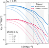 |
Fig. 1. Effective volume as a function of co-moving scale probed by AGNs and clusters (solid and dashed lines, respectively) in the eROSITA all-sky survey. The thicker the line, the better the quality of photo z. The grey band illustrates the scales where the BAO feature is prominent, and the vertical dashed line shows the position of the first peak. |
We therefore expect that both tracers suffer significantly from the loss of the photometric redshift precision and that the AGN and cluster samples would provide roughly comparable results and complement each other.
3. Modelling details
In this section, we illustrate our calculations of redshift distributions and number counts (Sect. 3.1), linear bias factors (Sect. 3.2), and the model for photometric redshift (Sect. 3.3).
3.1. X-ray luminosity functions
To the power spectrum shape, we need to know the space number densities of AGNs and clusters. With the knowledge of the X-ray luminosity function (XLF) of AGN ϕ(logL, z) and the flux limit of the survey, we calculated the distribution of AGNs with redshift. We used the XLF measured in Hasinger et al. (2005) with an exponential cutoff for z > 2.7 (Brusa et al. 2009); for details of calculations, see Kolodzig et al. (2013b).
The shape of the AGN XLF is the following:
![Mathematical equation: $$ \begin{aligned} \phi (L,z) = K_0 \left[ \left( \frac{L}{L_*} \right)^{\gamma _1} + \left( \frac{L}{L_*} \right)^{\gamma _2} \right]^{-1}\times e(L,z), \end{aligned} $$](/articles/aa/full_html/2023/01/aa44658-22/aa44658-22-eq7.gif)
where factor
 (1)
(1)
and cutoff redshift
 (2)
(2)
All parameters were taken from Hasinger et al. (2005), Table 5, LDDE model. The cutoff over redshift 2.7 is done as in Kolodzig et al. (2013b), i.e. ϕ(L, z)→ϕ(L, 2.7) × 100.43(2.7 − z) for z > 2.7.
The redshift distribution n(z), per deg2, is found as
where  is the differential co-moving volume, S is the flux limit of the survey (we adopt 10−14 erg s−1 cm−2), and the smallest observed luminosity Lmin at given redshift z is found as
  (rL is the luminosity distance). The k correction was done assuming a photon index of Γ = 1.9 and no absorption. We multiply the XLF by a factor of 1.3 to match the predicted sky number density of AGNs at a flux limit of 10−14 erg s−1 cm−2 with observations (i.e. ∼90 AGN/deg2; see e.g., Georgakakis et al. 2008).
The resulting AGN distribution is shown in Fig. 2 (panel A). The distribution peaks at z ≈ 1 and yields ≈2474000 AGN on 65.8% of the sky. This sky fraction corresponds to the extragalactic sky |b|> 15 deg. During the calculations of the effective volume in the previous section, the spatial number density of objects was found as  .
.
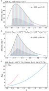 |
Fig. 2. Panels a, b: redshift distributions of AGN and cluster tracers. The black dashed line in each panel shows the total distribution of objects, while solid lines show the distributions of objects in photo-z bins (the corresponding vertical stripes show the boundaries of the bins in the photo-z space). The parameters for the photometric redshift scatter are shown in each panel. Panel c: effective linear bias factors of tracer populations as a function of z. |
To calculate the distribution of clusters of galaxies, we invoke the halo model approach. We start from the halo mass function n(M, z) of Tinker et al. (2008) and the fixed mass-luminosity relation of X-ray clusters calibrated in Vikhlinin et al. (2009a, Eq. (22))10. We used k correction assuming the thermal plasma model apec with temperature from Vikhlinin et al. (2009a, Table 3, free slope). The minimum mass for integration is taken as 5 × 10¹³h−1 M⊙ 11 since the ML relation is not well-known for lower masses. The redshift distribution is then found as
where, as before, Mmin(S, z) is the minimum observable mass at a given redshift, and Mmax is the maximum mass considered (1016h−1 M⊙). As the limiting flux we assume 4.4 × 10⁻¹⁴ erg s−1 cm−2 (for extended source detection, see Pillepich et al. 2012, Fig. 4).
Such a flux limit produces the redshift distribution shown in panel b) in Fig. 2, with the break at z ≈ 0.3 due to the minimum mass cut. On 65.8% of the sky, one would detect ≈93 400 clusters, with ≈900 of them at z > 1. Approximately 52 200 would have masses of M > 1014h−1 M⊙ , and 3100 clusters with M > 3 × 10¹⁴h−1 M⊙.
3.2. Linear bias factors
Active galactic nuclei and clusters live in dark matter halos. Halos are biased tracers of the underlying dark matter distribution, and they are more clustered.
The bias factors of X-ray-selected AGNs at different redshifts were measured with XMM-Newton data (Allevato et al. 2011) and were found to be consistent with the biasing of dark matter halos with the mass similar to that of the galaxy group, MDMH ∼ 1013 h−1 M⊙. We therefore used the model (fitting formulae) of Tinker et al. (2010) for the bias beff(z) of dark matter halos with mass of 2 × 10¹³h−1 M⊙. The bias is shown in panel c) of Fig. 2.
For X-ray clusters, we used the halo model with effective bias given by the average bias of halos weighed with their number density:
We show the effective bias of the cluster population in Fig. 2, panel c. At the peak redshift of the sample, the bias factor is ∼3. This is consistent with the bias measurements with the two-point correlation functions of ∼200 X-ray-selected galaxy clusters from the XMM-Newton XXL survey (Marulli et al. 2018). We limited our calculations for clusters of galaxies by a redshift of 0.8, as explained in Sect. 4. Correspondingly, we do need to construct a bias model for clusters beyond this redshift value.
3.3. Photometric redshift model
Photometric redshifts have poorer accuracy than redshifts based on spectroscopic data. However, it is compensated by the possibility to estimate redshifts for a much larger number of objects. A common approach to analysing photometric-redshift data sets is to bin objects in the redshift space so that one ‘integrates out’ the effects of photo-z errors. The width of the bins is chosen to be a few times the photo-z scatter at a given z. The true underlying distribution of redshifts (spec-z) would be smoothed in those bins by random errors (i.e. scatter zspec − zphot). We used the model of Hütsi et al. (2014) for Gaussian photometric redshift errors (see their Eq. (7)) with two parameters: σ0, which controls the scatter, and ffail – the catastrophic errors fraction. The smoothed shape of the ith redshift bin n(i) ( ) is given by
![Mathematical equation: $$ \begin{aligned} n^{(i)}(z)=n(z)&\left[\left(1-f_{\text{ fail}}\right) \frac{{\text{ erf}}\left(\frac{z_{\mathrm{p} _{2}}^{(\mathrm{i} )}-z}{\sqrt{2} \sigma (z)}\right)-{\text{ erf}}\left(\frac{z_{\mathrm{p} _{1}}^{(\mathrm{i} )}-z}{\sqrt{2} \sigma (z)}\right)}{1+{\text{ erf}}\left(\frac{z}{\sqrt{2} \sigma (z)}\right)}\right.\\&\left.+f_{\text{ fail} } \frac{z_{p_{2}}^{(i)}-z_{p_{1}}^{(i)}}{z_{p}^{\max }}\right], \end{aligned} $$](/articles/aa/full_html/2023/01/aa44658-22/aa44658-22-eq17.gif)
where σ(z)=σ0(1 + z) is the scatter and  is the maximum redshift of the sample.
The diluted bins of the photometric redshift selection of AGNs or clusters for fiducial values of parameters σ0 and ffail are shown in Fig. 2 on panels a) and b) with coloured solid lines. The coloured vertical strips correspond to the bin’s borders in photo-z space, and the solid line of the respective colour shows the true underlying distribution in spec-z space. As the redshift bin width, we use Δz = σ(z) at a given redshift if not stated otherwise. We illustrate the effect of photometric redshift errors in Fig. 3, where we plot the dilution of a redshift bin for various values of σ0.
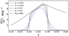 |
Fig. 3. Effect of photometric redshift errors on the redshift distribution of clusters of galaxies. The black dashed line shows the true distribution of clusters of galaxies over redshift. Thick solid lines show the observed distribution of clusters from the redshift bin 0.2 < z < 0.3 over photometric redshift for various values of σ0. The value of ffail is fixed at 0.05. |
Multi-wavelength data and the availability of rich spectroscopic information for large samples of objects allow efficient training of the models for source classification and photo-z evaluation. The SRGz machine learning system for classification and photometric redshift estimation is being developed by the Russian eROSITA consortium (Meshcheryakov et al., in prep.; see also Borisov et al. 2022; Belvedersky et al. 2022). SRGz is capable of determining photometric redshift probability density distribution of individual X-ray-selected AGNs with an accuracy better than σ0 ∼ 0.05 and the outlier fraction better than ∼10%. The accuracy of photo-z for galaxy clusters is nearly an order of magnitude better. In our analysis, we assumed that the photometric redshift error and fraction of catastrophic failures are known. These quantities and their redshift dependence are usually provided by the photometric redshift estimation code, based on the analysis of verification samples of objects whose redshifts are measured in spectroscopic observations. Our approach is similar, for example, to that used in Sereno et al. (2015). In the calculations below, we assumed the photo-z accuracy that is within the reach of the current version of the SRGz system.
4. Angular power spectrum and Fisher matrices
In this section, we describe the computation of angular power spectra (Sect. 4.1) and the calculation of Fisher matrices (Sect. 4.2).
4.1. Angular power spectrum
The angular power spectrum (APS) is a Fourier counterpart of the two-point angular correlation function. The benefit of using angular correlations is that one does not assume fiducial cosmology to analyse data.
The angular power spectrum of sources in i and jth redshift bins is calculated as follows:
where P(k, z = 0) is the matter 3d power spectrum at present time and  is a projection kernel of bin i. Secondly, we use
where r is a comoving radial distance, jℓ is the spherical Bessel function of order ℓ, f(i) is the normalised redshift distribution of ith bin, and g and beff are linear growth and bias factors, respectively.
Calculations of angular power spectra are done in CAMB and include the effects of redshift space distortions. The matter power spectrum is calculated by CAMB in the linear regime, while bias factors and redshift distributions are found as described in Sect. 3. We applied the Limber approximation (Simon 2007) at ℓ > 110 for both tracers. We used logarithmic bins in ℓ. A minimum multipole number, ℓ = 10, is used in all calculations due to the effects of the sky mask at lower multipoles. To not include non-linear effects in our analysis, we restricted ℓ < 500 (150) for AGN (cluster) samples (Kolodzig et al. 2013a; Hütsi et al. 2014). For the same reason, we used 0.5 (0.1) as the minimum redshift of a cosmological sample of AGN (clusters), whilst the maximum is 2.5 (0.8) due to the scarcity of objects at higher redshifts.
We used the following analytical formula for the Gaussian covariance matrix of angular power spectra:
with fsky being the fraction of the sky observed and Cij including the shot noise (1/N, where N is a surface density in the bin) if i = j. We treated partial sky coverage lightly with the factor fsky, whereas in reality the covariance between different modes would be introduced, especially for sky masks of complex shape. In the case of extragalactic sky |b|> 15° considered here, this effect can be neglected in this calculation.
To accelerate computations, we ignored cross-correlation between the bins that are spaced far apart (more than 3σ(z)). We remind the reader that the width of the redshift bin Δz is adjusted so that Δz = σ0(1 + z) for given photo-z scatter parameter σ0 unless stated otherwise.
4.2. Fisher matrix
We made use of the angular power spectra to derive errors in the determination of cosmological parameters with the Fisher matrix formalism.
Fisher matrices approximate the posterior distribution of the parameters of interest with multidimensional Gaussian distribution (Tegmark 1997; Tegmark et al. 1997; Dodelson 2003). We used the following formula for a Fisher matrix, assuming a Gaussian distribution of data points and constant covariance:
where Fi, j is a Fisher matrix, i, j are the indices of cosmological parameters of interest, Cℓ is a data vector, and Covℓ is data covariance. Our model includes all five cosmological parameters of flat ΛCDM: dark matter density fraction Ωc, baryon density fraction Ωb, reduced Hubble constant h, slope of primordial power spectrum ns, and the amplitude parameter σ8. Derivatives and covariance matrices were calculated in fiducial cosmology. We transformed the Fisher matrices so that instead of dark matter density Ωc, we used matter density Ωm = Ωc + Ωb, and we added priors to the matrix if needed (Coe 2009).
We found derivatives numerically using NUMDIFFTOOLS library12 with the jacobian of data vector calculated with step 5 × 10⁻⁴ and two-point central finite difference.
We do not include uncertainties of the redshift distribution n(z), bias beff(z), or M-L relation for clusters of galaxies in our simulations. We assumed that these quantities would be measured from the eROSITA all-sky survey with sufficient accuracy. In particular, as it was demonstrated in Kolodzig et al. (2013b), Comparat et al. (2019), the AGN XLF and bias b(z) will be accurately measured from the all-sky survey data. The M-L relation for clusters of galaxies also plays an important role in cosmological measurements with clusters (e.g., Pillepich et al. 2012). To this end, eROSITA is planned to measure this relation with high precision in the dedicated pointed phase after the all-sky survey ends.
After the Fisher matrix Fi, j is calculated, its inverse can be used as the covariance matrix of the parameters, from which one obtains marginalised errors (Tegmark et al. 1997; Coe 2009). In Appendix A, we compare the marginalised errors and credibility contours returned by the Fisher analysis and by the Markov chain Monte Carlo (MCMC) algorithm of posterior sampling and demonstrate that they produce consistent results.
In Fig. 4, we show the angular power spectrum examples for AGNs and clusters. In addition, we show logarithmic derivatives with respect to all cosmological parameters.
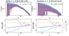 |
Fig. 4. Example of angular power spectra of AGNs (left panels) and clusters (right panels). In the top panels, the auto-spectrum of the first redshift bin is shown in blue (bin 0.9 < z < 0.99 for AGNs and 0.40 < z < 0.41 for clusters), and the cross-spectra of the first redshift bin with the second bin (0.99 < z < 1.09 for AGNs and 0.41 < z < 0.43 for clusters) in red. Horizontal lines show the level of Poisson noise for auto-spectra. In the bottom panels, the derivatives of those power spectra (solid and dashed lines, respectively) are shown with respect to parameters in the plot’s legend. Parameters of photometric redshift errors are σ0 = 0.05 and 0.01, ffail = 0.05 and 0.02 for AGNs and clusters, respectively. |
5. Forecast results
In the following section, we describe the main results of the paper: the significance of BAO detection in AGN and cluster distributions (Sect. 5.1) and the forecast on the cosmological constraining power of SRG/eROSITA samples of AGN and clusters of galaxies (Sect. 5.2).
To investigate the impact of photo-z errors, we used a grid of parameters, σ0 and ffail: σ0 = 0.005, 0.01, 0.015, 0.02, 0.03, 0.05, 0.07, 0.1, 0.2, 0.3 and ffail = 0.01, 0.02, 0.05, 0.1, 0.2 for clusters, and we did the same for AGNs, except for the AGNs we did not do calculations for: σ0 = 0.005 and 0.01. Redshift bin sizes are Δz = σ0(1 + z) except for the case of σ0 = 0.005, where we used redshift bins Δz = 1.3 × σ0(1 + z) to reduce the size of the matrices involved. We assumed the sky survey of fsky = 0.658 down to fluxes of 10−14 erg s−1 cm−2 (4.4 × 10⁻¹⁴ erg s−1 cm−2) and used objects in the redshift range of 0.5 < z < 2.5 (0.1 < z < 0.8) for AGNs (clusters). The total cosmological sample size would be ≈1.97 million AGNs and ≈88 000 clusters.
5.1. Baryon acoustic oscillations
We start from the question of whether BAOs would be detectable in the distribution of AGNs and clusters depending on the quality of photo z. A similar task was done in Hütsi et al. (2014) for the AGN population.
For BAO detection, we used the following technique: given the smooth model for the 3D matter power spectrum (template without BAO wiggles, NW superscript) we find the χ2 difference between data vectors Cℓ for a model with and without BAOs (i.e. confidence in units of σ):
As for the calculations of BAO significance, we used angular power spectra calculated by the CCL library (in contrast to the CAMB calculations done in the remainder of the paper) and compare the APS obtained with the matter power spectrum of Eisenstein and Hu, with and without wiggles (Eisenstein & Hu 1998) in Limber approximation.
The results of the exercise are presented in Fig. 5. We show contours of the significance of BAO detection as a function of both σ0 and ffail, along with cross-sections of such a surface with planes of constant σ0 or ffail.
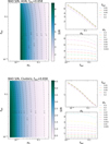 |
Fig. 5. Significance of BAO detection (S/N) in the sample of AGNs (top sub-figure) and clusters (bottom). In the left panel, the contours of significance are shown as a function of photo-z accuracy for parameters σ0 and ffail. In the right panels, the cross-sections with constant ffail (top) and σ0 (bottom) are shown. |
One can immediately see that in our regime for both tracers the photo-z scatter parameter has a greater impact on the performance (BAO detectability) than the catastrophic error fraction. Namely, the decrease of σ0 from 0.1 to 0.03 leads to the increase in the significance of BAO detection from ∼3σ to ∼6σ (assuming ffail = 0.01 for the AGN sample). Our results are in line with the work of (Hütsi et al. 2014; see their Fig. 7), notwithstanding the difference in implementation. For the AGN sample, the BAO significance achieves ∼7 − 8σ if σ0 = 0.015 (1.5%), but for a more realistic σ = 0.03 (3%) the figure is ∼5 − 6σ with little dependence on ffail. For clusters with σ0 = 0.005 (0.5%, which is quite a reasonable accuracy level of photo-z for clusters), the significance is ∼4 − 5σ.
Overall, we conclude that the detection of BAOs with photometric-quality z is plausible for both AGNs and clusters. The comparable statistical significance of BAO detection in both samples is also consistent with our expectation from the preliminary analysis based on effective volumes (Sect. 2).
5.2. Cosmological parameters
For each configuration of the photo-z quality, we calculated the Fisher matrix F of the cosmological parameters and the information content number called the figure of merit (FoM):
Hence, for every pair σ0,ffail, one obtains a Fisher matrix and the FoM.
Before we proceed with the effects of photo-z quality on the forecast, we show one example for the case σ0 = 0.03, 0.005 and ffail = 0.1, 0.01 for AGNs and clusters, respectively (see Fig. 6). We added a relatively weak Gaussian prior (0.1) to parameter h for this illustration. The value in parentheses is the standard deviation of the prior distribution and is indicated for other priors in the rest of the paper.
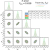 |
Fig. 6. Expected error ellipses of cosmological parameters from the analysis of AGNs and galaxy clusters in the complete eROSITA all-sky survey. Photometric redshift quality σ0 = 0.03, 0.005 and ffail = 0.1, 0.01 for AGNs and clusters, respectively. Prior 0.1 on h is added to the Fisher matrix. The corner plot shows the results derived from the Fisher matrix of clusters (blue), AGNs (orange), and combined (green) samples. The table shows the percentage errors on the parameters and the value for the FoM. |
We show expected error ellipses from the analysis of both samples separately and combined (i.e. adding two Fisher matrices). The figure also shows the table with the expected marginalised error percentages. Both AGNs and cluster samples give comparable errors on all the cosmological parameters. More importantly, the combination of AGN with clusters increases the FoM of the former by 0.6. This is due to the partial alleviation of the parameter degeneracy.
The parameter σ8 is well constrained because the error on the amplitude of the signal directly yields the constraints on the amplitude of fluctuations σ8. Parameters Ωc and ns have a level of accuracy better than ∼5% because they control the overall shape of the matter power spectrum and the prior added to h, which lifted the degeneracy with ns and Ωc. Ωb is not well constrained since the significance of baryonic effects on the angular power spectrum is limited.
We made such a forecast for each combination of photo-z precision parameters and condense the result in Fig. 7 using FoM as the proxy for the quality of the forecast. We assumed no priors for this calculation.
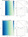 |
Fig. 7. Quality of cosmological constraints (FoM) in the sample of AGNs (top sub-figure) and clusters (bottom). In the left panel, the contours of quality are shown as a function of photo-z parameters σ0 and ffail. In the right panels, the cross-sections with constant ffail (top) and σ0 (bottom) are shown. |
As with BAOs, photo-z scatter σ0 affects the analysis quality dramatically, while ffail has a less profound influence on the result. For instance, a decrease of σ0 from 0.1 to 0.03 increases the FoM from ∼8.5 to ∼10 for AGNs with ffail = 0.01. For clusters FoM ∼ 6.5 with σ0 = 0.05 and FoM ∼ 9 if σ0 = 0.005. We conclude that the quality of cosmological analysis pivots on the σ0 parameter.
Table 1 shows the quality of the forecast for several cases of photometric redshift parameters. For a ‘conservative’ case, we chose the following parameters: σ0 = 0.01, 0.05 and ffail = 0.02, 0.1 for clusters and AGNs, respectively. For an ‘optimistic’ case, we choose σ0 = 0.005, 0.03 and ffail = 0.01, 0.1. We show options without prior information, with a wide prior on the reduced Hubble constant h (0.1) and, in particular, the prior knowledge of parameters h (0.0054) and ns (0.0042) derived from the Planck CMB experiment data (CMB+lensing, see Table 1 in Planck Collaboration VI 2020, last column). This demonstrates that the combination of the LSS probed by eROSITA and the independent data from other experiments may significantly enhance the resulting constraints.
SRG/eROSITA forecasts.
6. Discussion
6.1. Comparison with dedicated cosmological surveys
6.1.1. BAO
In Sect. 5.1, we predict that assuming realistic accuracy of photo-z determination – σ0 = 0.03 and 0.005 for AGNs and clusters, respectively, significant baryonic oscillations would be detected in the SRG/eROSITA all-sky survey in the distribution AGNs (redshift range of 0.5 < z < 2.5, about 2 million sources) and clusters of galaxies (redshift range 0.1 < z < 0.8, about 90 000 sources). Those figures are to be compared with the progress made so far in detecting the baryonic features at other wavelengths and using other LSS tracers.
Baryon acoustic oscillation peaks in galaxy distribution were detected for the first time in SDSS data (Eisenstein et al. 2005; Hütsi 2006) and have been routinely observed ever since (Ross et al. 2015; Alam et al. 2021).
There are many detections of BAOs with spectroscopic quality information at different redshifts. SDSS galaxies observed in the Baryon Oscillation Spectroscopic Survey (BOSS13) provide BAO detection in the redshift range of 0.2 < z < 0.75 from the sample of 1.2 million galaxies (Alam et al. 2017). The extended BOSS programme (eBOSS14) pushed the redshift range further, 0.6 < z < 1.1, with ∼400 k luminous red galaxies and ∼200 k emission line galaxies (Gil-Marín et al. 2020; Raichoor et al. 2021; Bautista et al. 2021; de Mattia et al. 2021). The SDSS observed the BAOs in the distribution of quasar (0.8 < z < 2.2 with ∼350 k objects) and Ly−α systems (210 k quasars at z > 2.1), see Neveux et al. (2020), du Mas des Bourboux et al. (2020), Hou et al. (2021).
Photometric data samples include the BAO detection in SDSS photometric catalogues (0.2 < z < 0.6, ∼600 k galaxies; Padmanabhan et al. 2007; Crocce et al. 2011; Seo et al. 2012). Recent results from the Dark Energy Survey provide evidence for baryonic wiggles in the distribution of ∼7 million galaxies with photo-z quality σ0 = 0.03 in redshift range 0.6 < z < 1.1 (Abbott et al. 2022b).
For clusters, BAO were tentatively (∼2σ) detected in SDSS photometric cluster catalogue with some ∼10 000 objects at z < 0.3 (Estrada et al. 2009; Hütsi 2010) for the first time. The significance of the detection has increased with the advent of better data, that is, ∼3.7σ detection with ∼80 k SDSS clusters at z < 0.5 with spectroscopic redshifts in the work of Hong et al. (2016); see also Moresco et al. (2021).
Considering all of the above, it is clear that the SRG/eROSITA sample of AGNs and clusters would provide sufficiently precise measurements of BAO (and the corresponding sound horizon scales) to expand and complement current experiments, and to provide a cross-check of clustering measurements. It may not be as efficient as SDSS or DES galaxies at a low-redshift regime (z < 0.6 − 0.7), but due to the satisfactory density of high-redshift objects, it may compete with BAO findings in eBOSS emission line galaxies and quasar distribution (see also Fig. 9 in Kolodzig et al. 2013a).
For clusters of galaxies, the SRG/eROSITA sample of X-ray-selected clusters would provide clear detection of BAO even with photometric quality redshifts with significance comparable to or exceeding the current statistical power of spectroscopic sample of clusters from SDSS.
6.1.2. Cosmological parameters
In Sect. 5.2, we forecast the precision of determination of cosmological parameters from the angular clustering of AGNs and clusters in the all-sky eROSITA survey. We show that under realistic assumptions about the accuracy of the photo-z one can achieve ∼1 − 20% marginalised errors on the cosmological parameters. The errors can be further reduced by a factor of ∼2 − 3 if using prior information from other experiments.
In Table 2 we compare SRG/eROSITA forecasts with other cosmological probes. In addition to the cosmological parameters discussed earlier, to ease comparison with other LSS surveys, we calculate uncertainty on the parameter of clustering amplitude S8 = σ8(Ωm/0.3)0.5. For comparison, in the two top lines of the table, we repeat the eROSITA combined AGN and clusters of galaxies forecast from the second half of Table 1. We show both forecasts made with and without the Planck priors h (0.0054) and ns (0.0042; Planck Collaboration VI 2020). The accuracy of cosmological parameter determination from the Planck data is shown in the third line of the table. Notably, the combined eROSITA sample in combination with Planck priors leads to improvement in the precision of determination for h, ns, and σ8 compared to Planck-only data.
Comparison of SRG/eROSITA forecasts with other cosmological probes.
Some of the LSS experiments use different LSS tracers (Alam et al. 2021). For example, Loureiro et al. (2019) used spectroscopic SDSS BOSS data of ∼1.3 million galaxies (0.15 < z < 0.8). The results (their Table 4) are listed in the fourth line in Table 2. X-ray samples, used without Planck priors, would have tighter errors on the parameter Ωm and S8, approximately similar uncertainty on Ωb and larger error margins for h and ns.
The ongoing Dark Energy Survey (DES) measures the shapes and positions of millions of galaxies. DES uses cosmic shear and clustering of galaxies as the effective cosmological probe of the matter fluctuation amplitude and density. We show their results (Y3, Table II in Abbott et al. 2022a) for flat ΛCDM from the DES data alone and with a combination of BAO and RSD measurements, supernovae, and CMB data. We see that SRG data alone provide better constraints on the matter density and perform worse for σ8 (we note in our forecast we that did not fix the other three parameters of the model). If compared with the combination of the DES and other probes, it is seen that the combination of eROSITA data and Planck prior for two parameters would perform comparably, having similar errors on h, and ns, larger errors on Ωm, Ωb, and S8, and a slightly smaller error on σ8. We also show the forecast results (Euclid Collaboration 2020) for the Euclid probe for the case of photometric galaxy clustering and weak lensing (their Table 9, optimistic settings for GCph+WL). As expected, Euclid will outperform eROSITA constraints without priors.
The above comparison demonstrates that samples of AGNs and clusters of galaxies from the SRG/eROSITA all-sky survey combined with the currently available photo-z estimates provide a sufficiently powerful cosmological LSS probe. They compete in statistical power with those derived from the dedicated cosmological large-scale structure surveys in the optical band. The statistical power of the eROSITA X-ray-selected samples will increase further if and when the accuracy of redshift determination achieves spectroscopic quality. This appears to be feasible, in principle, for clusters of galaxies that require the acquisition of ∼105 optical spectra. For AGNs, where ∼106 new optical spectra need to be obtained, this may be a more difficult task for the more distant future.
The calculations for cluster mass function were performed in Pillepich et al. (2012). We used the results for the fixed M-L relation for clusters of galaxies. They took the accuracy of photo-z into account by setting the redshift bin width at 0.05(1 + z) and the assumed sky coverage of fsky = 0.658, and they also used the Fisher matrix formalism. Comparing the last row of Table 2 with the first two rows and with Table 1, one can conclude that the cluster mass function is an equally important cosmological tool. When both are used without any priors, the mass-function-based measurement would be ∼5 times more accurate in measuring Ωm than the LSS-based one (which is to be expected). However, all other cosmological parameters are determined more accurately, by a factor of ∼1.5 − 3.5 in the LSS-based measurement (Clusters+AGN). Expressed in terms of the FoM, the cluster-mass function is expected to achieve FoM ≈ 10.1, which should be compared with FoM ≈ 9.8 − 10.4 for an LSS-based measurement (Table 1). The power of the cluster-mass-function method increases significantly when combined with the Planck priors.
Finally, it should be noted that the cluster-mass function is prone to systematic errors in mass determination, whereas the LSS-based measurement does not include systematic uncertainties of comparable amplitude (at least for AGNs) and therefore should be more robust. As discussed in Pillepich et al. (2012), the FoM of cosmological analysis degrades dramatically when the uncertainty in the M-L relation is included.
6.2. Dependence on the parameters of the all-sky survey
The SRG satellite performs a full scan of the sky in six months (Sunyaev et al. 2021), and it is planned to conduct eight all-sky surveys in the course of the mission. After the 4.4 already completed surveys, eROSITA achieved the record all-sky sensitivity of ∼15 times better than that reached in the previous all-sky survey performed by the ROSAT satellite in 1990 (Truemper 1982; Voges et al. 1999). It is therefore interesting to access the quality of cosmological measurements that can be achieved before the completion of the full survey.
To this end, we reran our calculations, changing the limiting flux of the survey to the values corresponding to two years of the survey (named eRASS4) and to three years (eRASS6). For point sources, these values are 1.45 × 10⁻¹⁴ (eRASS4) and 1.25 × 10⁻¹⁴ (eRASS6) erg s−1 cm−2, see (Kolodzig et al. 2013b). Changing the limiting flux affects the redshift distribution of tracer objects and, more importantly, their number density within redshifts of interest. For eRASS4,6,8 the number of sources is 1 051 773, 1 346 620, and 1 914 915, respectively (0.5 < z < 2.5). In Table 3, the forecast (with a wide prior in h and photo-z parameters σ0 = 0.03 and ffail = 0.1) is shown for these limiting fluxes. FoM values between eRASS4 and eRASS8 differ by 0.8, and the errors on the cosmological parameters increase by a factor of ∼1.5 − 2.
SRG/eROSITA forecasts for different survey parameters.
We also investigated the impact of the survey area on the forecast. We started by considering the case when only data from half of the extragalactic sky is used in calculations. We neglected the effects of the mode coupling in angular power spectra of half-sky masked data and simply change the sky area surveyed by a factor of two. In addition, we present a forecast for the survey with the area of 9000 deg2, which approximately corresponds to the footprint of the SDSS survey where the model of photo z would be better calibrated (at least for the AGN sample).
The scaling of Fisher matrices with fsky is trivial, Fi, j ∝ fsky, hence the marginalised errors scale as the inverse square root of the sky area. We illustrate in Table 3 the results for the fiducial eRASS8 AGN setup and show errors on cosmological parameters obtained for different sky areas used in the analysis. It can be seen that for the one half of the extragalactic sky  the results differ from the all-extragalactic case by a factor of
  , and the FoM differs by 0.75, whereas for the 9k deg2 case the errors are larger by approximately a factor of two, and the FoM value is smaller by 1.2.
7. Conclusions
We investigated the potential of X-ray-selected samples of AGNs and clusters of galaxies (to be) detected in the SRG/eROSITA all-sky survey to serve as a cosmological probe. We focused on the ability to detect BAOs and to constrain cosmological parameters under the assumption of the availability of photometric redshifts of realistically achievable quality. Our main results are given in Sects. 5.1 and 5.2.
Using the model of Hütsi et al. (2014) of photometric redshift scatter, we show that for both BAOs and the cosmological forecast, the redshift scatter parameter σ0 has more influence on the quality of cosmological constraints than the fraction of catastrophic errors ffail (Figs. 5 and 7)
We demonstrate that under reasonable assumptions regarding the quality of photo z (σ0 = 0.03 and 0.005 for AGNs and clusters of galaxies, respectively), it is possible to detect BAOs with a significance level of ∼5 − 6σ and ∼4 − 5σ in the distribution of AGNs and clusters, respectively. This is comparable with the BAO detections in large-scale structure surveys for galaxies and clusters (Sect. 6.1.1).
A Fisher matrix analysis of angular power spectra under the same assumptions yields the following: (i) a joint analysis of AGNs and cluster data alleviates some of the degeneracies and reduces errors on the cosmological parameters by a factor of ∼1.5 (Fig. 6); (ii) solely X-ray data constrain cosmological parameters with the accuracy in the ∼5 − 25% range without priors and in the ∼0.5 − 10% range with Planck priors (Table 1); (iii) X-ray-selected samples of SRG/eROSITA AGNs, and clusters of galaxies used alone or in combination with other data provide a powerful cosmological probe that represents stiff competition for the dedicated cosmological surveys such as SDSS or DES (Sect. 6.1.2 and Table 2).
Comparing with the results of Pillepich et al. (2012), we conclude that cosmological measurements based on the mass function of clusters of galaxies are expected to provide an ∼5 times more accurate measurement of Ωm than the LSS-based one. However, all other cosmological parameters are determined by a factor of ∼1.5 − 3.5 more accurately in the clustering-based measurement of AGNs and clusters of galaxies. Both methods give comparable values of the FoM (Tables 1 and 2).
We investigated the dependence of our forecasts on the survey parameters – its area and depth (Sect. 6.2, Table 3)15. We demonstrate16 that even with incomplete sky coverage or limited exposure SRG/eROSITA all-sky survey data17 still produce competitive results.
We ignore the scatter in this relation for simplicity, but uncertainties in this relation have a profound effect on the cosmological analysis, see Pillepich et al. (2012).
5 × 10¹³ h−1 M⊙ = 7.14 × 10¹³ M⊙ in our fiducial cosmology.
Acknowledgments
We are grateful to the referee for useful comments which improved the presentation of findings. SDB acknowledges support from and participation in the International Max-Planck Research School (IMPRS) on Astrophysics at the Ludwig-Maximilians University of Munich (LMU). SDB acknowledges partial support by the subsidy 671-2020-0052 allocated to Kazan Federal University for assignments in scientific activities. MG and RS acknowledge the partial support of this research by grant 21-12-00343 from the Russian Science Foundation. Software: CAMB (Lewis & Challinor 2011), CCL (Chisari et al. 2019), NumPy (Harris et al. 2020), Matplotlib (Hunter 2007), SciPy (Virtanen et al. 2020), Pandas (The pandas development team 2020), ChainConsumer, COBAYA (Torrado & Lewis 2021), AstroPy (Astropy Collaboration 2018), HEALPix (Górski et al. 2005), HEALPy (Zonca et al. 2019). The code used to produce the results of the paper would be available shortly after the publication. Data: no data is used for this paper.
References
- Abbott, T. M. C., Aguena, M., Alarcon, A., et al. 2022a, Phys. Rev. D, 105, 023520 [CrossRef] [Google Scholar]
- Abbott, T. M. C., Aguena, M., Allam, S., et al. 2022b, Phys. Rev. D, 105, 043512 [CrossRef] [Google Scholar]
- Alam, S., Ata, M., Bailey, S., et al. 2017, MNRAS, 470, 2617 [Google Scholar]
- Alam, S., Aubert, M., Avila, S., et al. 2021, Phys. Rev. D, 103, 083533 [NASA ADS] [CrossRef] [Google Scholar]
- Allen, S. W., Evrard, A. E., & Mantz, A. B. 2011, ARA&A, 49, 409 [Google Scholar]
- Allevato, V., Finoguenov, A., Cappelluti, N., et al. 2011, ApJ, 736, 99 [NASA ADS] [CrossRef] [Google Scholar]
- Allevato, V., Viitanen, A., Finoguenov, A., et al. 2019, A&A, 632, A88 [NASA ADS] [CrossRef] [EDP Sciences] [Google Scholar]
- Astropy Collaboration (Price-Whelan, A. M. et al.) 2018, AJ, 156, 123 [Google Scholar]
- Bautista, J. E., Paviot, R., Vargas Magaña, M., et al. 2021, MNRAS, 500, 736 [Google Scholar]
- Belvedersky, M. I., Meshcheryakov, A. V., Medvedev, P. S., & Gilfanov, M. R. 2022, Astron. Lett., 48, 109 [NASA ADS] [CrossRef] [Google Scholar]
- Beutler, F., Blake, C., Colless, M., et al. 2011, MNRAS, 416, 3017 [NASA ADS] [CrossRef] [Google Scholar]
- Blake, C., Kazin, E. A., Beutler, F., et al. 2011, MNRAS, 418, 1707 [NASA ADS] [CrossRef] [Google Scholar]
- Borisov, V., Meshcheryakov, A., & Gerasimov, S. 2022, in Astronomical Data Analysis Software and Systems XXX, ASP Conf. Ser., 532, 231 [NASA ADS] [Google Scholar]
- Brandt, W. N., & Hasinger, G. 2005, ARA&A, 43, 827 [NASA ADS] [CrossRef] [Google Scholar]
- Brusa, M., Comastri, A., Gilli, R., et al. 2009, ApJ, 693, 8 [Google Scholar]
- Chisari, N. E., Alonso, D., Krause, E., et al. 2019, ApJS, 242, 2 [Google Scholar]
- Coe, D. 2009, ArXiv e-prints [arXiv:0906.4123] [Google Scholar]
- Cole, S., Percival, W. J., Peacock, J. A., et al. 2005, MNRAS, 362, 505 [Google Scholar]
- Comparat, J., Merloni, A., Salvato, M., et al. 2019, MNRAS, 487, 2005 [Google Scholar]
- Crocce, M., Gaztañaga, E., Cabré, A., Carnero, A., & Sánchez, E. 2011, MNRAS, 417, 2577 [NASA ADS] [CrossRef] [Google Scholar]
- de Mattia, A., Ruhlmann-Kleider, V., Raichoor, A., et al. 2021, MNRAS, 501, 5616 [NASA ADS] [Google Scholar]
- Dodelson, S. 2003, Modern Cosmology (Amsterdam, Netherlands: Academic Press) [Google Scholar]
- du Mas des Bourboux, H., Rich, J., & Font-Ribera, A., et al. 2020, ApJ, 901, 153 [CrossRef] [Google Scholar]
- Eisenstein, D. J., & Hu, W. 1998, ApJ, 496, 605 [Google Scholar]
- Eisenstein, D. J., Zehavi, I., Hogg, D. W., et al. 2005, ApJ, 633, 560 [Google Scholar]
- Estrada, J., Sefusatti, E., & Frieman, J. A. 2009, ApJ, 692, 265 [NASA ADS] [CrossRef] [Google Scholar]
- Euclid Collaboration (Blanchard, A. et al.) 2020, A&A, 642, A191 [NASA ADS] [CrossRef] [EDP Sciences] [Google Scholar]
- Georgakakis, A., Nandra, K., Laird, E. S., Aird, J., & Trichas, M. 2008, MNRAS, 388, 1205 [Google Scholar]
- Gil-Marín, H., Bautista, J. E., Paviot, R., et al. 2020, MNRAS, 498, 2492 [Google Scholar]
- Górski, K. M., Hivon, E., Banday, A. J., et al. 2005, ApJ, 622, 759 [Google Scholar]
- Harris, C. R., Millman, K. J., van der Walt, S. J., et al. 2020, Nature, 585, 357 [NASA ADS] [CrossRef] [Google Scholar]
- Hasinger, G., Miyaji, T., & Schmidt, M. 2005, A&A, 441, 417 [NASA ADS] [CrossRef] [EDP Sciences] [Google Scholar]
- Hong, T., Han, J. L., & Wen, Z. L. 2016, ApJ, 826, 154 [NASA ADS] [CrossRef] [Google Scholar]
- Hou, J., Sánchez, A. G., Ross, A. J., et al. 2021, MNRAS, 500, 1201 [Google Scholar]
- Hunter, J. D. 2007, Comput. Sci. Eng., 9, 90 [NASA ADS] [CrossRef] [Google Scholar]
- Hütsi, G. 2006, A&A, 449, 891 [NASA ADS] [CrossRef] [EDP Sciences] [Google Scholar]
- Hütsi, G. 2010, MNRAS, 401, 2477 [CrossRef] [Google Scholar]
- Hütsi, G., Gilfanov, M., Kolodzig, A., & Sunyaev, R. 2014, A&A, 572, A28 [NASA ADS] [CrossRef] [EDP Sciences] [Google Scholar]
- Kaiser, N. 1987, MNRAS, 227, 1 [Google Scholar]
- Kolodzig, A., Gilfanov, M., Sunyaev, R., Sazonov, S., & Brusa, M. 2013a, A&A, 558, A89 [NASA ADS] [CrossRef] [EDP Sciences] [Google Scholar]
- Kolodzig, A., Gilfanov, M., Hütsi, G., & Sunyaev, R. 2013b, A&A, 558, A90 [NASA ADS] [CrossRef] [EDP Sciences] [Google Scholar]
- Kolodzig, A., Gilfanov, M., Hütsi, G., & Sunyaev, R. 2017, MNRAS, 466, 3035 [NASA ADS] [CrossRef] [Google Scholar]
- Kolodzig, A., Gilfanov, M., Hütsi, G., & Sunyaev, R. 2018, MNRAS, 473, 4653 [NASA ADS] [CrossRef] [Google Scholar]
- Lewis, A., & Bridle, S. 2002, Phys. Rev. D, 66, 103511 [Google Scholar]
- Lewis, A., & Challinor, A. 2011, Astrophysics Source Code Library [record ascl:1102.026] [Google Scholar]
- Loureiro, A., Moraes, B., Abdalla, F. B., et al. 2019, MNRAS, 485, 326 [NASA ADS] [CrossRef] [Google Scholar]
- Marulli, F., Veropalumbo, A., Sereno, M., et al. 2018, A&A, 620, A1 [NASA ADS] [CrossRef] [EDP Sciences] [Google Scholar]
- Merloni, A., Predehl, P., Becker, W., et al. 2012, ArXiv e-prints [arXiv:1209.3114] [Google Scholar]
- Moresco, M., Veropalumbo, A., Marulli, F., Moscardini, L., & Cimatti, A. 2021, ApJ, 919, 144 [NASA ADS] [CrossRef] [Google Scholar]
- Mountrichas, G., Georgakakis, A., Menzel, M. L., et al. 2016, MNRAS, 457, 4195 [NASA ADS] [CrossRef] [Google Scholar]
- Neveux, R., Burtin, E., de Mattia, A., et al. 2020, MNRAS, 499, 210 [NASA ADS] [CrossRef] [Google Scholar]
- Padmanabhan, N., Schlegel, D. J., Seljak, U., et al. 2007, MNRAS, 378, 852 [NASA ADS] [CrossRef] [Google Scholar]
- Padmanabhan, N., Xu, X., Eisenstein, D. J., et al. 2012, MNRAS, 427, 2132 [Google Scholar]
- The pandas development team 2020, https://doi.org/10.5281/zenodo.3509134 [Google Scholar]
- Peebles, P. J. E., & Yu, J. T. 1970, ApJ, 162, 815 [NASA ADS] [CrossRef] [Google Scholar]
- Percival, W. J., Reid, B. A., Eisenstein, D. J., et al. 2010, MNRAS, 401, 2148 [Google Scholar]
- Pillepich, A., Porciani, C., & Reiprich, T. H. 2012, MNRAS, 422, 44 [Google Scholar]
- Planck Collaboration VI. 2020, A&A, 641, A6 [NASA ADS] [CrossRef] [EDP Sciences] [Google Scholar]
- Predehl, P., Andritschke, R., Arefiev, V., et al. 2021, A&A, 647, A1 [EDP Sciences] [Google Scholar]
- Raichoor, A., de Mattia, A., Ross, A. J., et al. 2021, MNRAS, 500, 3254 [Google Scholar]
- Ross, A. J., Samushia, L., Howlett, C., et al. 2015, MNRAS, 449, 835 [NASA ADS] [CrossRef] [Google Scholar]
- Seo, H.-J., Ho, S., White, M., et al. 2012, ApJ, 761, 13 [NASA ADS] [CrossRef] [Google Scholar]
- Sereno, M., Veropalumbo, A., Marulli, F., et al. 2015, MNRAS, 449, 4147 [NASA ADS] [CrossRef] [Google Scholar]
- Simon, P. 2007, A&A, 473, 711 [NASA ADS] [CrossRef] [EDP Sciences] [Google Scholar]
- Sunyaev, R. A., & Zeldovich, Y. B. 1970, Ap&SS, 7, 3 [NASA ADS] [Google Scholar]
- Sunyaev, R., Arefiev, V., Babyshkin, V., et al. 2021, A&A, 656, A132 [NASA ADS] [CrossRef] [EDP Sciences] [Google Scholar]
- Tegmark, M. 1997, Phys. Rev. D, 55, 5895 [NASA ADS] [CrossRef] [Google Scholar]
- Tegmark, M., Taylor, A. N., & Heavens, A. F. 1997, ApJ, 480, 22 [NASA ADS] [CrossRef] [Google Scholar]
- Tegmark, M., Blanton, M. R., Strauss, M. A., et al. 2004, ApJ, 606, 702 [Google Scholar]
- Tinker, J., Kravtsov, A. V., Klypin, A., et al. 2008, ApJ, 688, 709 [Google Scholar]
- Tinker, J. L., Robertson, B. E., Kravtsov, A. V., et al. 2010, ApJ, 724, 878 [NASA ADS] [CrossRef] [Google Scholar]
- Torrado, J., & Lewis, A. 2019, Astrophysics Source Code Library [record ascl:1910.019] [Google Scholar]
- Torrado, J., & Lewis, A. 2021, JCAP, 2021, 057 [Google Scholar]
- Truemper, J. 1982, Adv. Space Res., 2, 241 [Google Scholar]
- Vikhlinin, A., Burenin, R. A., Ebeling, H., et al. 2009a, ApJ, 692, 1033 [Google Scholar]
- Vikhlinin, A., Kravtsov, A. V., Burenin, R. A., et al. 2009b, ApJ, 692, 1060 [Google Scholar]
- Virtanen, P., Gommers, R., Oliphant, T. E., et al. 2020, Nat. Methods, 17, 261 [Google Scholar]
- Voges, W., Aschenbach, B., Boller, T., et al. 1999, A&A, 349, 389 [NASA ADS] [Google Scholar]
- Zonca, A., Singer, L., Lenz, D., et al. 2019, J. Open Source Software, 4, 1298 [Google Scholar]
Appendix A: Fisher formalism and MCMC method
There are conditions to be met for the Fisher analysis to yield realistic constraints on the parameters of the model. One such condition is that the posterior probability distribution is a multi-dimensional Gaussian distribution. This is clearly not the case for cosmological models since there are non-linear degeneracies in the parameters. However, one might hope that the resulting errors would be small so that the linear approximation holds and the Fisher matrix method indeed produces a sound forecast.
To test the method, we made a Fisher forecast for the case of AGN (eRASS8, fsky = 0.658) with follow-up quality σ0 = 0.03 and ffail = 0.1 and priors 0.05 on h and 0.01 on ns. Then, we used COBAYA18 code for Bayesian analysis in Cosmology (Torrado & Lewis 2019, 2021) and their implementation of the MCMC Metropolis sampler (Lewis & Bridle 2002) to probe the posterior. We assumed a Gaussian likelihood with appropriate priors and made ’data’ from our data vector, loaded a covariance matrix, and then ran chains until the convergence. In Fig. A.1, we visualise the probability contours of two methods and in Table A.1, we compare the marginalised 68% credible intervals. One can see that under our assumptions the Fisher forecast produces contours and errors consistent with the result of the full MCMC treatment of the problem. Based on the results of this and other similar tests we chose to use the Fisher matrix formalism, which is significantly computationally faster than MCMC, as our baseline tool.
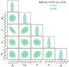 |
Fig. A.1. Error ellipses of cosmological parameter estimation from the angular power spectra for the case of AGNs (σ0 = 0.03, ffail = 0.1) with priors. Blue dashed ellipses are the result of the Fisher forecast, whilst the shaded regions show the result of MCMC sampling done in COBAYA. Darker areas correspond to the 68% probability contour, and the lighter areas to 95%. On the diagonal of the plot grid, the marginalised histograms of the corresponding parameter are shown. The Fisher formalism provides a forecast in good agreement with the MCMC results. |
Table corresponding to Fig. A.1. The values of the mean of the parameters and corresponding marginalised errors are shown for the MCMC method and the Fisher forecast.
All Tables
Table corresponding to Fig. A.1. The values of the mean of the parameters and corresponding marginalised errors are shown for the MCMC method and the Fisher forecast.
All Figures
|
Fig. 1. Effective volume as a function of co-moving scale probed by AGNs and clusters (solid and dashed lines, respectively) in the eROSITA all-sky survey. The thicker the line, the better the quality of photo z. The grey band illustrates the scales where the BAO feature is prominent, and the vertical dashed line shows the position of the first peak. |
| In the text | |
|
Fig. 2. Panels a, b: redshift distributions of AGN and cluster tracers. The black dashed line in each panel shows the total distribution of objects, while solid lines show the distributions of objects in photo-z bins (the corresponding vertical stripes show the boundaries of the bins in the photo-z space). The parameters for the photometric redshift scatter are shown in each panel. Panel c: effective linear bias factors of tracer populations as a function of z. |
| In the text | |
|
Fig. 3. Effect of photometric redshift errors on the redshift distribution of clusters of galaxies. The black dashed line shows the true distribution of clusters of galaxies over redshift. Thick solid lines show the observed distribution of clusters from the redshift bin 0.2 < z < 0.3 over photometric redshift for various values of σ0. The value of ffail is fixed at 0.05. |
| In the text | |
|
Fig. 4. Example of angular power spectra of AGNs (left panels) and clusters (right panels). In the top panels, the auto-spectrum of the first redshift bin is shown in blue (bin 0.9 < z < 0.99 for AGNs and 0.40 < z < 0.41 for clusters), and the cross-spectra of the first redshift bin with the second bin (0.99 < z < 1.09 for AGNs and 0.41 < z < 0.43 for clusters) in red. Horizontal lines show the level of Poisson noise for auto-spectra. In the bottom panels, the derivatives of those power spectra (solid and dashed lines, respectively) are shown with respect to parameters in the plot’s legend. Parameters of photometric redshift errors are σ0 = 0.05 and 0.01, ffail = 0.05 and 0.02 for AGNs and clusters, respectively. |
| In the text | |
|
Fig. 5. Significance of BAO detection (S/N) in the sample of AGNs (top sub-figure) and clusters (bottom). In the left panel, the contours of significance are shown as a function of photo-z accuracy for parameters σ0 and ffail. In the right panels, the cross-sections with constant ffail (top) and σ0 (bottom) are shown. |
| In the text | |
|
Fig. 6. Expected error ellipses of cosmological parameters from the analysis of AGNs and galaxy clusters in the complete eROSITA all-sky survey. Photometric redshift quality σ0 = 0.03, 0.005 and ffail = 0.1, 0.01 for AGNs and clusters, respectively. Prior 0.1 on h is added to the Fisher matrix. The corner plot shows the results derived from the Fisher matrix of clusters (blue), AGNs (orange), and combined (green) samples. The table shows the percentage errors on the parameters and the value for the FoM. |
| In the text | |
|
Fig. 7. Quality of cosmological constraints (FoM) in the sample of AGNs (top sub-figure) and clusters (bottom). In the left panel, the contours of quality are shown as a function of photo-z parameters σ0 and ffail. In the right panels, the cross-sections with constant ffail (top) and σ0 (bottom) are shown. |
| In the text | |
|
Fig. A.1. Error ellipses of cosmological parameter estimation from the angular power spectra for the case of AGNs (σ0 = 0.03, ffail = 0.1) with priors. Blue dashed ellipses are the result of the Fisher forecast, whilst the shaded regions show the result of MCMC sampling done in COBAYA. Darker areas correspond to the 68% probability contour, and the lighter areas to 95%. On the diagonal of the plot grid, the marginalised histograms of the corresponding parameter are shown. The Fisher formalism provides a forecast in good agreement with the MCMC results. |
| In the text | |
Current usage metrics show cumulative count of Article Views (full-text article views including HTML views, PDF and ePub downloads, according to the available data) and Abstracts Views on Vision4Press platform.
Data correspond to usage on the plateform after 2015. The current usage metrics is available 48-96 hours after online publication and is updated daily on week days.
Initial download of the metrics may take a while.