| Issue |
A&A
Volume 667, November 2022
|
|
|---|---|---|
| Article Number | A131 | |
| Number of page(s) | 14 | |
| Section | Extragalactic astronomy | |
| DOI | https://doi.org/10.1051/0004-6361/202244563 | |
| Published online | 17 November 2022 | |
Understanding if molecular ratios can be used as diagnostics of AGN and starburst activity: The case of NGC 1068
1
Leiden Observatory, Leiden University, PO Box 9513, 2300 RA Leiden, The Netherlands
e-mail: butterworth@strw.leidenuniv.nl, viti@strw.leidenuniv.nl, holdship@strw.leidenuniv.nl
2
Department of Physics and Astronomy, University College London, Gower St., London WC1E 6BT, UK
3
Observatorio Astronómico Nacional (OAN-IGN)-Observatorio de Madrid, Alfonso XII, 3, 28014 Madrid, Spain
Received:
21
July
2022
Accepted:
9
September
2022
Context. Molecular line ratios, such as HCN(1−0)/HCO+(1−0) and HCN(4−3)/CS(7−6), are routinely used to identify active galactic nuclei (AGN) activity in galaxies. Such ratios are, however, hard to interpret as they are highly dependent on the physics and energetics of the gas, and hence can seldom be used as a unique, unambiguous diagnostic.
Aims. We used the composite galaxy NGC 1068 as a “laboratory” to investigate whether molecular line ratios between HCN, HCO+, and CS are useful tracers of AGN-dominated gas and determine the origin of the differences in such ratios across different types of gas. Such a determination will enable a more rigorous use of such ratios.
Methods. First, we empirically examined the aforementioned ratios at different angular resolutions to quantify correlations. We then used local thermodynamic equilibrium (LTE) and non-LTE analyses coupled with Markov chain Monte Carlo sampling in order to determine the origin of the underlying differences in ratios.
Results. We propose that at high spatial resolution (< 50 pc) the HCN(4−3)/CS(2−1) is a reliable tracer of AGN activity. We also find that the variations in ratios are not a consequence of different densities or temperature but of different fractional abundances, yielding to the important result that it is essential to consider the chemical processes at play when drawing conclusions from radiative transfer calculations.
Conclusions. From analyses at varying spatial scales, we find that previously proposed molecular line ratios, as well as a new one, have varying levels of consistency. We also determine from an investigation of radiative transfer modelling of our data that it is essential to consider the chemistry of the species when reaching conclusions from radiative transfer calculations.
Key words: astrochemistry / ISM: molecules / galaxies: active / galaxies: ISM / galaxies: Seyfert / galaxies: starburst
© J. Butterworth et al. 2022
 Open Access article, published by EDP Sciences, under the terms of the Creative Commons Attribution License (https://creativecommons.org/licenses/by/4.0), which permits unrestricted use, distribution, and reproduction in any medium, provided the original work is properly cited.
This article is published in open access under the Subscribe-to-Open model. Subscribe to A&A to support open access publication.
1. Introduction
The gas and dust present in the interstellar medium (ISM) within galaxies is not homogeneous; star formation, supernovae events, and active galactic nuclei (AGN) activity may all greatly alter the ISM (see e.g. Meijerink & Spaans 2005; Bayet et al. 2009; Watanabe et al. 2014). In particular, recent studies of nearby external galaxies have shown that the molecular ISM varies at a parsec, as well as at kiloparsec scales, with evidence of different gas components being traced by different molecular species or rotational transitions (Scourfield et al. 2020). The non-homogeneity of the ISM has been observed in galaxies of different types, such as starburst (SB) galaxies (Meier et al. 2015), AGN-dominated galaxies (Audibert et al. 2019), and ultra-luminous infrared galaxies (ULIRGs; Imanishi et al. 2018a).
Molecular line ratio diagnostics are often used to investigate the physics and chemistry of the ISM in all of these environments. For example, as the gas chemistry located in the central, nuclear regions of galaxies is believed to be dominated by X-rays produced by the AGN, in so-called X-ray dominated regions (XDRs), the molecular content of the ISM surrounding such nuclei will greatly differ from that in starburst regions (Usero et al. 2004; García-Burillo et al. 2010). Hence, line ratios of specific molecules have been proposed as indicators of certain energetic or physical processes, for example HCN/HCO+ as a tracer of AGNs (Loenen et al. 2007), HCN/HNC as a mechanical heating tracer (Hacar et al. 2020), and HCN/CO as a density tracer (Leroy et al. 2017). In particular, the “submillimeter-HCN diagram”, first proposed in Izumi et al. (2013) and later expanded upon in Izumi et al. (2016), is a very notable example of the use of molecular line ratios as a probe of AGN-galaxies; this diagram makes use of two line ratios, HCN(4−3)/HCO+(4−3) and HCN(4−3)/CS(7−6), where all of the molecules involved are considered tracers of dense gas. Izumi et al. (2016) observed a clear trend that AGNs, including the Seyfert composite galaxy NGC 1068, tend to show higher HCN/HCO+ and/or HCN/CS than in SB galaxies as long as the observations were at high enough spatial resolutions to separate energetically discrete regions. Izumi et al. (2016) propose a scenario where it is the high temperature that is responsible for the HCN enhancement, whereby neutral-neutral reactions with high reaction barriers are enhanced (Harada et al. 2010), thus leading to the possible enhancement of HCN and the depletion of HCO+ via newly available formation and destruction paths, respectively. However, while of course higher gas temperatures are expected in AGN-dominated regions, these are not unique to these environments, as starburst regions and/or regions where outflows dominate can also harbour high enough temperatures for such enhancement to occur. Additionally, the higher temperatures could increase HCN excitation, relative to HCO+ and CS, without necessarily changing their relative abundances (Imanishi et al. 2018a). Finally, infrared radiative pumping is also a possible explanation of the HCN intensity enhancement relative to HCO+ and CS. Infrared pumping is a result of the emission of 14 μm infrared photons due to the presence of hot dust around AGN. These photons vibrationally excite HCN to the ν2 = 1 state. Upon de-exciting from this state back to the vibrational ground state, ν = 0, the HCN line intensities are thus pumped to higher fluxes (Imanishi et al. 2018a). However, we note that it is also not unlikely that the 12 μm infrared photons can similarly vibrationally excite HCO+, thus nullifying the extent of this effect (Imanishi et al. 2016).
In fact, while Miyamoto et al. (2017) observed a similar variation consistent with the “submillimeter-HCN” diagram between the circumnuclear disc (CND) and the star-forming ring of the Seyfert 2 galaxy NGC 613, indicating that the enhancement of HCN may indeed be more prominent in AGN-dominated gas, some studies have observed HCN/HCO+ enhancements in SB galaxies similar to those observed in AGNs (Harada et al. 2018; König et al. 2018). Furthermore, a statistical study by Privon et al. (2020) surveying a sample of 58 local luminous infrared galaxies and ULIRGs, concluded that an enhancement in the HCN/HCO+(1−0) line ratio could not be shown to be correlated to the AGN activity. They also concluded that HCN/HCO+ ratios are not a dependable method for finding AGN regions in galaxies. Finally, from a chemical point of view the HCN/HCO+ ratio has be shown to be highly dependent on numerous factors, such as density, temperatures, and radiation fields, and cannot alone be used as a unique diagnostic of AGN-dominated galaxies (Viti 2017).
It is clear that for a meaningful analysis of molecular line ratios, one first needs to know whether there are there unique molecular ratios at a specific spatial resolution that trace distinct types of gas and energetics associated with AGN- and SB-dominated galaxies. Additionally, one needs to know if molecular ratios obtained at different spatial resolutions yield different trends.
In order to obtain these answers, we performed a multi-scale investigation into the use of molecular line ratios as tracers, particularly of AGN versus SB activity, by using the galaxy NGC 1068 as a “laboratory”. NGC 1068 is a Seyfert 2 barred spiral galaxy; it is also the archetypal composite AGN/SB galaxy. Its close proximity (∼14 Mpc) and significant brightness (LBol ≈2.5−3.0 × 10¹¹ L⊙; Bland-Hawthorn et al. 1997; Bock et al. 2000) enable studies at many different resolutions, down to parsec scales, with 1″ corresponding to ∼70 pc for reference (García-Burillo et al. 2014, 2016, 2019; Viti et al. 2014; Gallimore et al. 2016; Imanishi et al. 2018b, 2020; Impellizzeri et al. 2019). In Sect. 2 we provide a summary of the data collated for this study. Section 3 presents an analysis of various molecular ratios at both high and low spatial resolution. In Sect. 4 we perform an LTE and non-LTE analysis of the line intensities used for the ratios in Sect. 3, in order to determine whether such an analysis is consistent with the trends implied by the ratios. We summarise our findings in Sect. 5.
2. Data
Despite the plethora of available published data focused on NGC 1068, within this study we focus on the dense gas tracers: HCN, HCO+, and CS. This focus is in an effort to validate previously proposed ratios and diagrams rather than to suggest new ones. We therefore searched published data for observations of these molecules in NGC 1068 and a summary of all of the data utilised within this study is provided in Table 1. Observations from multiple instruments were used, including interferometric observations from Atacama Large Millimetre/submillimetre Array (ALMA) and Plateau de Bure Interferometer (PdBI), and single dish observations from the 15 m diameter James Clerk Maxwell Telescope (JCMT).
Studies.
To supplement these data, we also re-analysed previously published data (Sánchez-García et al. 2022) of HCN(1−0) and HCO+(1−0) emission observations. Both lines were observed with ALMA’s Band 3 receiver during cycle 2 (project-ID: 2013.1.00055.S; PI: S. García-Burillo).
The phase tracking centre was set to  ,
,  (J2000 reference system, as used throughout the paper) in each case, the position of the galaxy’s centre in the SIMBAD Astronomical Database, from the Two-Micron All-Sky Survey (2MASS; Skrutskie et al. 2006). This is offset relative to the galaxy AGN at
  ,
,  by < 1″, and corresponds to a peak in CO emission (García-Burillo et al. 2014). Initial reduction of the data was carried out using the ALMA reduction package CASA (McMullin et al. 2007), and then exported to PYTHON for plotting, making use of the Matplotlib and Astropy. The 1σ threshold was determined in CASA by calculating the rms of the signal over an area towards the centre of the galaxy in a channel with no line detection. The angular resolution obtained using uniform weighting was ∼0.7″ × 0.5″ at a position angle of −86° in the data cube. The conversion factor between Jy beam−1 and K is 32 K Jy beam−1.
2.1. Moment 0 maps
Figures and 2 show the velocity integrated maps at the original spatial resolution for HCO+(1−0) and HCN(1−0), respectively. As can be seen in these two figures, HCN(1−0) is observed to be significantly more prominent in the CND regions than the equivalent HCO+(1−0) emission.
The structure of the CND ring as observed in previous observations (García-Burillo et al. 2014, 2019) at similarly high resolution in CO, CS, and higher J-transitions of HCN and HCO+, is observed in these intensity maps, with the east and west knots showing particularly prominent emission in these lines. The two knots are connected by “bridges” of emission, within which the CND-N and CND-S regions are located. Emission in these “bridges” is seen to be significantly more prominent in HCN(1−0) rather than HCO+(1−0). Within the SB ring regions, however, HCO+ is observed to be most prominent, the notable exception being NSB-c at which significant HCN emission is seen to dominate over the respective HCO+ emission; the implications of this are further elaborated upon in the following section. As both lines were taken from the same data set at the same resolution, their respective rms are both approximately σ = 16 K km s−1 at this resolution.
Moment 0 maps for the remaining high-resolution data can be found in the following papers: the CS(2−1) moment 0 map in Fig. A.1 of Scourfield et al. (2020); CS(7−6) in Fig. A.3 of Scourfield et al. (2020); HCO+(4−3) in Fig. 8 of García-Burillo et al. (2014); a zoomed-in moment 0 map of HCN(4−3) is presented in Fig. 8 of García-Burillo et al. (2014), with a zoomed-out equivalent also available in Appendix B.1, with an accompanying HCO+(4−3) plot in Appendix B.2.
2.2. Comparison between observations
The range of transitions from multiple studies will allow us to approach the analysis of NGC 1068 from both a large-scale view, using the low spatial resolution detections of single dish instruments, and a more zoomed-in one, provided to us via interferometric instruments. The different spatial resolutions make it necessary to ensure that only similarly obtained detections are compared. This is especially true for the higher-resolution observations that cover only a small area of the galaxy. For those observations, the variance over even small distances can be large. An example of such small-scale variation in emission can be seen in the CND in Fig. 1.
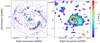 |
Fig. 1. HCO+J(1−0) velocity-integrated moment map. The beam size is shown by the orange ellipse. The lowest contour displayed is 3σ, where σ = 16 K km s−1, with the following contours corresponding to 5σ, 10σ, 20σ, 30σ, 45σ, and 70σ. |
We therefore grouped our data in two ways. Firstly, the archival data were grouped by spatial resolution. Within these groupings, there were variations of resolution of up to a factor of two. Therefore, we deconvolved the intensities by assuming the observation with the lowest resolution was the source size and using the equation
where ISource is the source averaged peak intensity, θs is the source size (as defined by the lowest-resolution observation in the category), θb is the beam size, and IBeam is the original intensity as defined in the archive or paper. This is similar to the approach taken in Kamenetzky et al. (2011), Aladro et al. (2013), Aladro et al. (2015) in order to account for the effect of beam dilution.
The high-resolution data were then further separated by the sub-region on which they were focused. For the low-resolution data, this was not a concern as each observation contained many sub-regions. We list each sub-region in Table 2. The regions in the CND and the SB ring observed within this report are consistent with those observed in Scourfield et al. (2020), with the exception of the region known as NSB-b, as none of the ratios investigated within this report have been observed at a consistent resolution for this region. We note that not all sub-regions listed in Table 2, and shown in Figs. and 2, have been observed at all resolutions for all molecules. As a result, some ratios in some regions are missing at certain resolutions (see Fig. 3). The region NSB-c possesses fewer observed ratios than the other regions, with just a single high-resolution observation (see Table 3). As a result it is not included in the RADEX fitting discussed later in this paper.
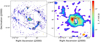 |
Fig. 2. HCN J(1−0) velocity-integrated moment map. The beam size is shown by the orange ellipse. The lowest contour displayed is 3σ, where σ = 16 K km s−1, with the following contours corresponding to 5σ, 10σ, 20σ, 30σ, 45σ, 70σ, 100σ, and 150σ. |
Names and coordinates of the sub-regions of interest across the CND and the SB ring.
3. Molecular line ratios
The combination of archival and new data allows us to investigate molecular line ratios that have been proposed as tracers of different regions as well as to propose a new tracer. In this section, we take an in-depth look at these ratios across the resolutions and sub-region groupings in order to determine which relationships stand up to scrutiny.
3.1. HCN/HCO+
HCN and HCO+ are both dense gas tracers, with HCN(1−0) and HCO+(1−0) having critical densities of ∼105 cm−3 and ∼5 × 104 cm−3 (at ∼10 K, Shirley 2015), respectively. The HCN(1−0)/HCO+(1−0) and HCN(4−3)/HCO+(4−3) ratios have both been proposed as tracers of AGN activity (Kohno 2005; Izumi et al. 2013). Therefore, in this section, we discuss each ratio in turn, with a particular focus on how well the ratio separates AGN regions from SB regions. All the ratios for NGC 1068 are presented in Figs. 3 and 4.
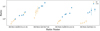 |
Fig. 3. High-resolution (∼40 pc scale) observations of the four ratios investigated in this paper, split into regions located in the CND and the SB ring. Values and uncertainties of the ratio values plotted here are given in Table 3. |
 |
Fig. 4. Data from Fig. 3 with the addition of lower-resolution data (see Table 1) for the two ratios that showed reasonable distinction between the CND and the SB ring regions. |
3.1.1. HCN(1−0)/HCO+(1−0)
An enhancement of HCN(1−0) relative to HCO+(1−0) or CO(1−0) has been proposed as an indicator of AGN activity (Imanishi et al. 2007; Krips et al. 2008; Davies et al. 2012). In fact, Kohno et al. (2001) proposed the HCN diagram; a diagnostic diagram to identify AGN galaxies using this line ratio and the ratio of HCN(1−0)/CO(1−0). However, as detailed in the introduction, some studies find high HCN(1−0)/HCO+(1−0) ratios in SB galaxies (Costagliola et al. 2011) and low values of this ratio in AGNs (Sani et al. 2012), which casts doubt on the use of this ratio to trace AGN activity. In the high-resolution archival data, as well as the new ALMA data we have collated, we typically observe the same distinction in this ratio as in other studies. We find that a HCN(1−0)/HCO+(1−0) ratio of greater than one is located in regions near the AGN, and a ratio less than one is found in those outside of the CND (see Fig. 3). Although it must be noted that at the X-ray matched position of the AGN, the sub-region denoted as AGN, the observed ratios are significantly lower than in the other CND regions, which may be consistent with the conclusion reached by Privon et al. (2020) that HCN(1−0)/HCO+(1−0) does not trace AGN activity directly. We also note that in García-Burillo et al. (2014) and Viti et al. (2014), large HCN(1−0)/HCO+(1−0) (as well as the ratio of higher J) was in fact associated with large scale shocks that were associated with the molecular outlfow, rather than XDR chemistry, a scenario also explored in García-Burillo et al. (2010). Recent galactic studies, such as the study into the prototypical shock region L1157-B1 in Lefloch et al. (2021), have shown a marked increase in HCN abundance relative to H2 in these environments, relative to pre-shock gas.
However, there are significant exceptions. Sub-region NSB-c is not associated with the AGN but has the second largest ratio value. We note, however, that all the lines detected in NSB-c are significantly weaker than those found in the other SB regions.
3.1.2. HCN(4−3)/HCO+(4−3)
Similar to the enhancement of HCN relative to HCO+ observed in their respective J = 1 − 0 transitions, Izumi et al. (2013) found a similar trend for the J = 4 − 3 transitions. This ratio has advantages over the J = 1 − 0 ratio as higher-resolution imaging is more easily achievable, it can be observed to higher distances (up to z ∼ 3 with ALMA), and the transitions have higher critical densities, resulting in lower contamination by foreground or other extended emission (Izumi et al. 2016). HCN(4−3) and HCO+(4−3) possess high and similar critical densities of ncrit, HCN(4 − 3) ≈ 8.5 × 106 cm−3 and ncrit, HCO+(4 − 3)∼106 cm3 (at ∼10 K, Shirley 2015), which means that they are more likely to trace the same component of the dense gas in any observed region.
Figure 3 seems to imply that this ratio does separate AGN and non-AGN regions in our high-resolution data. Moreover, once low-resolution data are included, the ratio continues to distinguish between regions (Fig. 4), albeit with a smaller gap between the two types of region. It must be noted, however, that for region NSB-c, both HCN(4−3) and HCO+(4−3) emission is below the 3σ threshold necessary to derive a reliable intensity ratio. Hence, we cannot be sure whether in NSB-c this ratio follows the same trend as HCN(1−0)/HCO+(1−0).
3.2. HCN/CS
CS is also a commonly used dense gas tracer; CS(1−0) has a critical density of ncrit ∼ 104 cm3 (Shirley 2015). Izumi et al. (2013) present the use of CS as opposed to HCO+ as the molecule with which the HCN enhancement should be measured because earlier studies had shown that the CS abundance varies little between active regions (e.g. near the AGN in the CND) and those in SB regions (Martín et al. 2008, 2009). For this reason, the HCN/CS ratio has been proposed as a possible starburst and AGN tracer. Under XDR conditions, the CS abundance should be unchanged but the HCN abundance is enhanced, leading to an enhancement in the ratio (Krieger et al. 2020).
3.2.1. HCN(4−3)/CS(7−6)
Izumi et al. (2013) state that the intensity ratio between HCN(J = 4 − 3) and CS(J = 7 − 6) was found to be high in AGN galaxies (> 12.7). HCN(4−3) has an excitation temperature of 42.53 K and a critical density of ≈107 cm−3. CS(7−6) has an excitation temperature of 65.8 K and a critical density of ≈106 cm−3 (at ∼10 K, Shirley 2015). Audibert et al. (2021) observed results consistent with those proposed by the Izumi papers in NGC 1808. Despite this, we find that, even at high spatial resolution, this ratio does not clearly distinguish the CND from the SB regions. Considering the uncertainty in the ratios that we calculated, there is significant overlap between the ratio values at positions in each region. Thus, one would not be able to reliably separate an unusually large SB ratio caused by a random error from a large ratio, due to the CND enhancement.
One possible reason for the failure of this ratio, given its previous success, is that Izumi et al. (2013, 2016) used lower-resolution observations than those used here. Hence, they may trace more extended regions. We indeed also typically find that the highest values for this ratio are obtained from the lower-resolution observations in our data. This point is shown quite clearly in Fig. 5, which is a recreation of the sub-millimetre-HCN diagram from Izumi et al. (2016) of the HCN(4−3)/HCO+(4−3) and the HCN(4−3)/CS(7−6) ratios.
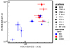 |
Fig. 5. Recreation of the sub-millimetre-HCN diagram from Izumi et al. (2016) using various resolution data across various sub-regions in NGC 1068. The shape of each marker denotes the region it corresponds to and the colour denotes the resolution. |
3.2.2. HCN(4−3)/CS(2−1)
We further investigated the HCN(4−3)/CS(2−1) ratio. For NSB-c, as before, we did not have a strong enough detection for HCN(4−3), and as such we could not derive this ratio for this region. Taking a 3σ upper limit for the HCN(4−3) in this sub-region, we obtained an upper limit for the HCN(4−3)/CS(2−1) ratio of ∼1.4, which is significantly lower than the those observed in the CND regions. Considering all the remaining regions, we find that at high spatial resolution, a clear distinction can be made between the CND and SB regions, as shown in Fig. 3.
This is not surprising if we consider the difference in the lines. The HCN(4−3) transition has an upper state energy of 43 K and a critical density of ∼8.5 × 106 cm−3, whilst the CS(2−1) transition has an upper state energy of 7 K and a critical density of 8 × 104 cm−3. Since the two transitions are likely to be excited under very different gas conditions, this ratio should be able to discriminate between SB and CND regions.
However, Fig. 4 shows that once lower-resolution observations are included, this ratio becomes less reliable. In particular, including low-resolution data adds an SB observation that is the second highest observation of this ratio.
4. Physical and chemical properties of NGC 1068
We have found that the ratio between HCN(4−3) and HCO+(4−3) clearly separates SB and AGN regions in our data. We have also found that the ratio between HCN(4−3) and CS(2−1) is reliable at high resolution. However, these are observed correlations with as yet undetermined underlying physical or chemical cause. In this section, we attempt to find that cause so that these ratios can be more robustly used to probe AGN regions.
To achieve this, we used radiative transfer modelling to infer the gas conditions and molecular column densities at each location for each resolution. We were then able to determine whether there are physical differences in excitation conditions between locations, differences in the underlying chemical abundances, or even a combination of the two as a result of shocks, or processes involving X-rays or cosmic rays. If it is the former, these ratios may only distinguish between regions insofar as the gas temperature and density are typically different. If it is the latter, more detailed chemical modelling is required to determine the cause of the chemical distinction.
4.1. LTE analysis
Using the observed line intensities from the archival data, we were able to estimate the column densities by assuming LTE and by using the same groupings of observations as discussed earlier, devolved to the lowest resolution of that group. The upper state column density of a molecular transition can be approximated to
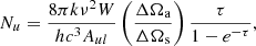
where W is the integrated line intensity, Aul is the Einstein A-coefficient, and τ is the optical depth, which we included as a correction factor for saturated lines. Ωa and Ωs are the solid angles of the antenna and the source, respectively, and together give the beam filling factor. Since we are investigating the regions themselves, we made the assumption that the source completely fills the beam, such that  .
.
We could then use these transition column densities to approximate the total column density of the emitting molecule, N, by using

where Z(T) is the partition function, gu is the statistical weight of level u, and Eu is the excitation energy of level u. To compute the partition function, we made use of molecular data from the Cologne Database for Molecular Spectroscopy (CDMS; Endres et al. 2016). We combined Eqs. (2) and (3) to produce an estimate of the column density for each molecule. We used temperatures in the range 50 K–400 K and computed the column density from each transition independently, with this range of temperatures being based upon previous modelling studies of these regions in Viti et al. (2014) and Izumi et al. (2016). We set τ = 0 for our lines, following the example of Krips et al. (2008). By following this procedure, we obtained a broad range of possible values for the column densities, which act as limits for the grid of radiative transfer models used to obtain non-LTE results in the next section. Table 4 shows the minimum and maximum LTE column density results for each molecule.
Lower and upper limits of column density calculated for each molecule assuming LTE.
4.2. Non-LTE analysis
In order to understand how the physical conditions of the CND regions and the SB regions relate to the possible tracers discussed in this paper, we compared the data with a grid of Large Velocity Gradient (LVG) models. We used RADEX for this task via the SpectralRadex python package1.
RADEX is a non-LTE radiative transfer code developed by van der Tak et al. (2007), which uses the escape probability method (Sobolev 1960). We assumed the sub-regions could be approximated as uniform spheres and computed the line intensities of each molecule for different physical parameters. To do this, we took collisional data between each molecule and H2 from the LAMDA database (Schöier et al. 2005).
We then ran a grid of physical parameters for each molecule. In this grid, we varied the physical parameters over the ranges summarised in Table 5. We based the gas density and kinetic temperature ranges on previous studies of NGC 1068 (Viti et al. 2014; Izumi et al. 2016), while the column density ranges were taken from the LTE analysis in Sect. 4.1. In addition to these parameters, we tried three line widths that cover ranges of typical line widths observed in the SB regions (50 km s−1) and the CND regions (150 km s−1; Scourfield et al. 2020).
Range of physical parameters over which the RADEX models were computed.
We used the resulting line intensities to compute the ratios that we have explored in this paper, namely: HCN(1−0)/HCO+(1−0), HCN(4−3)/HCO+(4−3), HCN(4−3)/CS(7−6), and HCN(4−3)/CS(2−1). We then fit these modelled ratios to their observed values by Markov chain Monte Carlo (MCMC) sampling the χ2 distribution of the parameters. For all parameter combinations, we computed the χ2 statistic:
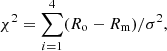
in order to compare goodness of fit. Ro and Rm are the observed and modelled ratios, respectively, and σ is the uncertainty in the observed ratio propagated from the uncertainty in the individual intensities. Assuming a uniform prior, sampling this distribution gives the posterior probability distribution of the parameters.
Our MCMC sampler uses 12 walkers, each performing 100 000 steps, to sample possible parameter combinations. We did this for all combinations of regions and resolutions with at least two of the investigated ratios. The joint posterior distributions of temperature and density are shown in Fig. A.1 for each of the available regions at the highest resolution (∼40 pc scale). Table 6 summarises the parameters of the MCMC fitting of the RADEX models over the entire parameter space for nine of the ten regions studied in Scourfield et al. (2020), with NSB-c being excluded due to a lack of observed ratios, as stated in Sect. 2.2. Neither the CND nor the SB ring regions can be reasonably constrained in the temperature or density planes, at least with regards to showing distinguishing qualities within these parameters. The only two regions in the CND where strong constraints on the gas density can be drawn are the east and west knot regions ( and
and  , respectively). Similarly the SB ring region, NSB-a, has a relatively highly constrained density of
  . The impact of resolution when it comes to the determination of temperature, density, and linewidth, with regards to each region, is negligible as a result of the fact that these parameters are not reasonably constrained at any resolution. However, it must be noted that the density becomes extensively less constrained for all regions as the resolution is diminished; this can be seen in Fig. A.2. Despite the lack of strong constraints, it is clear from this that the best-fit gas densities and temperatures are generally quite similar between the CND and the SB regions. This strongly suggests that we cannot link the difference in ratios between SB and CND regions to either of these quantities. While the results for the temperature are relatively unconstrained, it is notable that the median values (at high resolution) for the SB region appear to be higher than those located in the CND, particularly those in the CND-N and CND-S. However, while typically the CND regions, by virtue of being located closer to the AGN, would be expected to have higher temperatures, it is possible to imagine a scenario of high SB activity that could lead to average temperatures of the order of ∼300 K (typical of galactic hot cores, e.g. Kaufman et al. 1998). On the other hand, we also note that there is significant uncertainty in these obtained temperature values.
Median, 16th, and 84th percentile parameter value results from the MCMC chains resulting from fitting to the observed ratios.
Figures A.3–A.5 display the 1 sigma ranges of the posterior distributions for the column densities of HCN, HCO+, and CS as a result of the ∼40 pc and ∼100 pc data. While there are some general trends towards lower (for HCN) or higher (for HCO+ and CS) column densities in the SB ring regions with respect to the CND regions, especially at the 40 pc scale, there is a significant overlap between the regions.
To account for the fact that the total H2 column density varies across individual regions, and thus may be obscuring an underlying HCN enhancement, we computed the posterior probability distributions of the ratios of the column densities. We did this by taking the ratio of the chains of column density samples for each region and resolution. The resulting 16th and 84th percentile limits of the three ratio distributions are shown in Fig. A.6. What we observe at our highest resolution is that the best fitting RADEX models typically have higher abundances of HCN relative to both HCO+ and CS within the AGN-dominated CND regions when compared to the best fitting models of the SB-dominated SB ring regions. This distinction is maintained somewhat in the lower-resolution (∼100 pc scale) data for HCN relative to HCO+, but not for HCN with respect to CS. The abundances of CS and HCO+ appear to cover relatively similar ranges, regardless of the region observed.
It is therefore the underlying ratio of the HCN/HCO+ and the HCN/CS abundances that distinguish the process characteristics of an AGN-dominated region or galaxy versus that of an SB-dominated region or galaxy. Thus, line ratios are only useful insofar as they probe the column density differences, and therefore multi-line multi-species observations coupled with chemical modelling will always be a more powerful, if not essential, method to discriminate and characterise different types of galaxies, while minimising degeneracy in radiative transfer modelling.
5. Summary and conclusion
By taking NGC 1068 as a “laboratory”, we have investigated whether molecular line ratios are useful tracers of AGN-dominated gas. More importantly we determined the origin of the differences in such ratios across different types of gas. Our main conclusions are the following:
-
For the HCN(1−0)/HCO+(1−0) and HCN(4−3)/CS(7−6) ratios, we observe an overlap in the observed ranges of these ratios between AGN-dominated and SB-dominated regions. For HCN(4−3)/CS(7−6) specifically, we notice that the range of values observed in each of the two types of regions overlapped significantly even at the highest spatial resolution.
-
The HCN(1−0)/HCO+(1−0) ratio first proposed in Kohno (2005) and then put into question by Privon et al. (2020) does appear to show an enhancement in the CND with respect to the SB ring regions for the majority of sub-regions; however, we found an ‘outlier’ in at least one SB region, (NSB-c).
-
HCN(4−3)/HCO+(4−3), on the other hand, seems to be distinctively higher in all the regions closer to the AGN position, at least at higher spatial resolutions. This distinction is even maintained when the ratio is viewed at lower-resolution scales, although the separation does decrease. It is important to note, however, that for NSB-c the HCN(4−3) and HCO+(4−3) lines are too weak, and thus we cannot confirm whether this ratio in this region conforms to the trend stated above.
-
When observed at high spatial resolution, we propose a new ratio as a reliable tracer of AGN activity: the HCN(4−3)/CS(2−1).
-
We investigated the origin of the differences in ratios and found that differences in gas densities and temperatures are not the cause of the differentiation. Upon computing the relative fractional abundances of HCN, HCO+, and CS, we in fact determined that these differences are a consequence of differences in chemical abundances. Hence, it is essential to consider the chemistry of the species (i.e. which chemical processes lead to such abundances) when drawing conclusions from radiative transfer calculations (Viti 2017).
-
As also noted in García-Burillo et al. (2014) and Viti et al. (2014) the elevated HCN(1−0)/HCO+(1−0) and HCN(4−3)/HCO+(4−3) ratios observed throughout the CND can be attributed to the molecular outflow observed in this region. As such, the contribution of mechanical heating and possible shock chemistry in the CND could be possible contributors to the observed HCN enhancement (Kelly et al. 2017; Huang et al. 2022).
In conclusion, we have attempted to evaluate the effectiveness of selected molecular line ratios as tracers of AGN versus SB activity in the galaxy NGC 1068. We have found that previously proposed ratios such as HCN(1−0)/HCO+(1−0) and HCN(4−3)/CS(7−6) do not appear to be sufficient, regardless of the spatial scale investigated, whereas HCN(4−3)/HCO+(4−3) HCN(4−3)/CS(2−1) may show promise at certain resolutions. However, follow up studies, especially of other nearby galaxies, are required in order to confirm our findings. Finally, we find that the observed variances in these ratios are a result of variances in the chemical abundances, and hence chemical modelling is necessary in order to determine the origin of the differences in ratios.
Acknowledgments
This work is part of a project that has received funding from the European Research Council (ERC) under the European Union’s Horizon 2020 research and innovation programme MOPPEX 833460. S.G.B. acknowledges support from the research project PID2019-106027GA-C44 of the Spanish Ministerio de Ciencia e Innovación. This paper makes use of the following ALMA data: (project-ID: 2013.1.00055.S; PI: S. García-Burillo). The published data displayed in the following papers were also used in this study: Sánchez-García et al. (2022), García-Burillo et al. (2008, 2014), Viti et al. (2014), Pérez-Beaupuits et al. (2009), Tan et al. (2018), Scourfield et al. (2020), Takano et al. (2014), Tacconi et al. (1997), Nakajima et al. (2015), Bayet et al. (2009). The authors would like to thank the anonymous referee for constructive comments that improved the original version of the paper.
References
- Aladro, R., Viti, S., Bayet, E., et al. 2013, A&A, 549, A39 [NASA ADS] [CrossRef] [EDP Sciences] [Google Scholar]
- Aladro, R., Martín, S., Riquelme, D., et al. 2015, A&A, 579, A101 [NASA ADS] [CrossRef] [EDP Sciences] [Google Scholar]
- Audibert, A., Combes, F., García-Burillo, S., et al. 2019, A&A, 632, A33 [NASA ADS] [CrossRef] [EDP Sciences] [Google Scholar]
- Audibert, A., Combes, F., García-Burillo, S., et al. 2021, A&A, 656, A60 [NASA ADS] [CrossRef] [EDP Sciences] [Google Scholar]
- Bayet, E., Viti, S., Williams, D. A., Rawlings, J. M. C., & Bell, T. 2009, ApJ, 696, 1466 [NASA ADS] [CrossRef] [Google Scholar]
- Bland-Hawthorn, J., Gallimore, J. F., Tacconi, L. J., et al. 1997, Astrophys. Space Sci., 248, 9 [NASA ADS] [CrossRef] [Google Scholar]
- Bock, J. J., Neugebauer, G., Matthews, K., et al. 2000, AJ, 120, 2904 [NASA ADS] [CrossRef] [Google Scholar]
- Costagliola, F., Aalto, S., Rodriguez, M. I., et al. 2011, A&A, 528, A30 [NASA ADS] [CrossRef] [EDP Sciences] [Google Scholar]
- Davies, R., Mark, D., & Sternberg, A. 2012, A&A, 537, A133 [NASA ADS] [CrossRef] [EDP Sciences] [Google Scholar]
- Endres, C. P., Schlemmer, S., Schilke, P., Stutzki, J., & Müller, H. S. 2016, J. Mol. Spectrosc., 327, 95 [NASA ADS] [CrossRef] [Google Scholar]
- Gallimore, J. F., Elitzur, M., Maiolino, R., et al. 2016, ApJ, 829, L7 [Google Scholar]
- García-Burillo, S., Combes, F., Graciá-Carpio, J., Usero, A., & Guélin, M. 2008, Ap&SS, 313, 261 [CrossRef] [Google Scholar]
- García-Burillo, S., Usero, A., Fuente, A., et al. 2010, A&A, 519, A2 [NASA ADS] [CrossRef] [EDP Sciences] [Google Scholar]
- García-Burillo, S., Combes, F., Usero, A., et al. 2014, A&A, 567, A125 [Google Scholar]
- García-Burillo, S., Combes, F., Ramos Almeida, C., et al. 2016, ApJ, 823, L12 [Google Scholar]
- García-Burillo, S., Combes, F., Ramos Almeida, C., et al. 2019, A&A, 632, A61 [Google Scholar]
- Hacar, A., Bosman, A. D., & van Dishoeck, E. F. 2020, A&A, 635, A4 [NASA ADS] [CrossRef] [EDP Sciences] [Google Scholar]
- Harada, N., Herbst, E., & Wakelam, V. 2010, ApJ, 721, 1570 [NASA ADS] [CrossRef] [Google Scholar]
- Harada, N., Sakamoto, K., Martín, S., et al. 2018, ApJ, 855, 49 [Google Scholar]
- Huang, K. Y., Viti, S., Holdship, J., et al. 2022, A&A, 666, A102 [NASA ADS] [CrossRef] [EDP Sciences] [Google Scholar]
- Imanishi, M., Nakanishi, K., Tamura, Y., Oi, N., & Kohno, K. 2007, ApJ, 134, 2366 [CrossRef] [Google Scholar]
- Imanishi, M., Nakanishi, K., & Izumi, T. 2016, AJ, 152, 218 [Google Scholar]
- Imanishi, M., Nakanishi, K., & Izumi, T. 2018a, ApJ, 856, 143 [Google Scholar]
- Imanishi, M., Nakanishi, K., Izumi, T., & Wada, K. 2018b, ApJ, 853, L25 [NASA ADS] [CrossRef] [Google Scholar]
- Imanishi, M., Nguyen, D. D., Wada, K., et al. 2020, ApJ, 902, 99 [CrossRef] [Google Scholar]
- Impellizzeri, C. M. V., Gallimore, J. F., Baum, S. A., et al. 2019, ApJ, 884, L28 [NASA ADS] [CrossRef] [Google Scholar]
- Izumi, T., Kohno, K., Martín, S., et al. 2013, PASJ, 65, 100 [NASA ADS] [Google Scholar]
- Izumi, T., Kohno, K., Aalto, S., et al. 2016, ApJ, 818, 42 [NASA ADS] [CrossRef] [Google Scholar]
- Kamenetzky, J., Glenn, J., Maloney, P. R., et al. 2011, ApJ, 731, 83 [NASA ADS] [CrossRef] [Google Scholar]
- Kaufman, M. J., Hollenbach, D. J., & Tielens, A. G. G. M. 1998, ApJ, 497, 276 [NASA ADS] [CrossRef] [Google Scholar]
- Kelly, G., Viti, S., García-Burillo, S., et al. 2017, A&A, 597, A11 [NASA ADS] [CrossRef] [EDP Sciences] [Google Scholar]
- Kohno, K. 2005, in The Evolution of Starbursts, eds. S. Hüttmeister, E. Manthey, D. Bomans, & K. Weis, AIP Conf. Ser., 783, 203 [Google Scholar]
- Kohno, K., Matsushita, S., Vila-Vilaró, B., et al. 2001, in The Central Kiloparsec of Starbursts and AGN: The La Palma Connection, eds. J. H. Knapen, J. E. Beckman, I. Shlosman, & T. J. Mahoney, ASP Conf. Ser., 249, 672 [NASA ADS] [Google Scholar]
- König, S., Aalto, S., Muller, S., et al. 2018, A&A, 615, A122 [NASA ADS] [CrossRef] [EDP Sciences] [Google Scholar]
- Krieger, N., Bolatto, A. D., Leroy, A. K., et al. 2020, ApJ, 897, 176 [Google Scholar]
- Krips, M., Neri, R., García-Burillo, S., et al. 2008, ApJ, 677, 262 [NASA ADS] [CrossRef] [Google Scholar]
- Lefloch, B., Busquet, G., Viti, S., et al. 2021, MNRAS, 507, 1034 [CrossRef] [Google Scholar]
- Leroy, A. K., Usero, A., Schruba, A., et al. 2017, ApJ, 835, 217 [NASA ADS] [CrossRef] [Google Scholar]
- Loenen, A. F., Baan, W. A., & Spaans, M. 2007, in Astrophysical Masers and their Environments, eds. J. M. Chapman, & W. A. Baan, 242, 462 [NASA ADS] [Google Scholar]
- Martín, S., Requena-Torres, M. A., Martín-Pintado, J., & Mauersberger, R. 2008, ApJ, 678, 245 [CrossRef] [Google Scholar]
- Martín, S., Martín-Pintado, J., & Mauersberger, R. 2009, ApJ, 694, 610 [CrossRef] [Google Scholar]
- McMullin, J. P., Waters, B., Schiebel, D., Young, W., & Golap, K. 2007, in Astronomical Data Analysis Software and Systems XVI, eds. R. A. Shaw, F. Hill, & D. J. Bell, ASP Conf. Ser., 376, 127 [Google Scholar]
- Meier, D. S., Walter, F., Bolatto, A. D., et al. 2015, ApJ, 801, 63 [NASA ADS] [CrossRef] [Google Scholar]
- Meijerink, R., & Spaans, M. 2005, A&A, 436, 397 [CrossRef] [EDP Sciences] [Google Scholar]
- Miyamoto, Y., Nakai, N., Seta, M., et al. 2017, PASJ, 69, 83 [CrossRef] [Google Scholar]
- Nakajima, T., Takano, S., Kohno, K., et al. 2015, PASJ, 67, 8 [NASA ADS] [CrossRef] [Google Scholar]
- Pérez-Beaupuits, J. P., Spaans, M., van der Tak, F. F. S., et al. 2009, A&A, 503, 459 [NASA ADS] [CrossRef] [EDP Sciences] [Google Scholar]
- Privon, G. C., Ricci, C., Aalto, S., et al. 2020, ApJ, 893, 149 [NASA ADS] [CrossRef] [Google Scholar]
- Sánchez-García, M., García-Burillo, S., Pereira-Santaella, M., et al. 2022, A&A, 660, A83 [NASA ADS] [CrossRef] [EDP Sciences] [Google Scholar]
- Sani, E., Davies, R. I., Sternberg, A., et al. 2012, MNRAS, 424, 1963 [NASA ADS] [CrossRef] [Google Scholar]
- Schöier, F. L., van der Tak, F. F. S., van Dishoeck, E. F., & Black, J. H. 2005, A&A, 432, 369 [Google Scholar]
- Scourfield, M., Viti, S., García-Burillo, S., et al. 2020, MNRAS, 496, 5308 [NASA ADS] [CrossRef] [Google Scholar]
- Shirley, Y. L. 2015, PASP, 127, 299 [Google Scholar]
- Skrutskie, M. F., Cutri, R. M., Stiening, R., et al. 2006, AJ, 131, 1163 [NASA ADS] [CrossRef] [Google Scholar]
- Sobolev, V. V. 1960, Moving Envelopes of Stars (Cambridge: Harvard University Press) [Google Scholar]
- Tacconi, L. J., Gallimore, J. F., Genzel, R., Schinnerer, E., & Downes, D. 1997, Ap&SS, 248, 59 [NASA ADS] [CrossRef] [Google Scholar]
- Takano, S., Nakajima, T., Kohno, K., et al. 2014, PASJ, 66, 75 [NASA ADS] [Google Scholar]
- Tan, Q.-H., Gao, Y., Zhang, Z.-Y., et al. 2018, ApJ, 860, 165 [NASA ADS] [CrossRef] [Google Scholar]
- Usero, A., García-Burillo, S., Fuente, A., Martín-Pintado, J., & Rodríguez-Fernández, N. J. 2004, A&A, 419, 897 [NASA ADS] [CrossRef] [EDP Sciences] [Google Scholar]
- van der Tak, F. F. S., Black, J. H., Schöier, F. L., Jansen, D. J., & van Dishoeck, E. F. 2007, A&A, 468, 627 [NASA ADS] [CrossRef] [EDP Sciences] [Google Scholar]
- Viti, S. 2017, A&A, 607, A118 [NASA ADS] [CrossRef] [EDP Sciences] [Google Scholar]
- Viti, S., García-Burillo, S., Fuente, A., et al. 2014, A&A, 570, A28 [NASA ADS] [CrossRef] [EDP Sciences] [Google Scholar]
- Watanabe, Y., Sakai, N., Sorai, K., & Yamamoto, S. 2014, ApJ, 788, 4 [NASA ADS] [CrossRef] [Google Scholar]
Appendix A: Additional figures
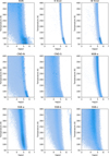 |
Fig. A.1. Resulting joint posterior distributions for temperature and density as produced for the high resolution (∼40 pc scale data) for the nine regions that have enough ratios to fit. The temperasture and density values shown in Table 6 are from distributions visualised in this plot. It must be noted that the median values of these distributions, as shown in Table 6, do not always correspond to the most densely populated areas of the corresponding plot. This is due to the extent of the posterior distribution in the temperature plane. |
 |
Fig. A.2. Resulting joint posterior distributions for temperature and density as produced for the lower resolution (∼100 pc scale data) for the six regions that have enough ratios to fit, at this lower resolution. |
 |
Fig. A.3. 16th to 84th percentile range of the MCMC for the column density of HCN, as found from fitting the observed ratios to those produced by RADEX models. |
 |
Fig. A.4. 16th to 84th percentile range of the MCMC for the column density of HCO+, as found from fitting the observed ratios to those produced by RADEX models. |
 |
Fig. A.5. 16th to 84th percentile range of the MCMC for the column density of CS, as found from fitting the observed ratios to those produced by RADEX models. |
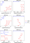 |
Fig. A.6. Produced relative fractional abundances of HCN, HCO+, and CS across the various regions in NGC 1068 at both the 40 pc and 100 pc scale. |
Appendix B: Additional moment 0 maps
B.1. HCN(4-3)
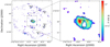 |
Fig. B.1. HCN J(4-3) velocity-integrated moment map. The beam size is shown by the orange ellipse. The lowest contour displayed is 3σ, where σ = 6.8 K km s−1, with the following contours corresponding to 5σ, 10σ, 20σ, 30σ, 45σ, 70σ, 100σ, and 150σ. |
B.2. HCO+(4-3)
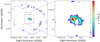 |
Fig. B.2. HCO+ J(4-3) velocity-integrated moment map. The beam size is shown by the orange ellipse. The lowest contour displayed is 3σ, where σ = 6.4 K km s−1, with the following contours corresponding to 5σ, 10σ, 20σ, 30σ, 45σ, 70σ, 100σ, and 150σ. |
All Tables
Names and coordinates of the sub-regions of interest across the CND and the SB ring.
Lower and upper limits of column density calculated for each molecule assuming LTE.
Median, 16th, and 84th percentile parameter value results from the MCMC chains resulting from fitting to the observed ratios.
All Figures
|
Fig. 1. HCO+J(1−0) velocity-integrated moment map. The beam size is shown by the orange ellipse. The lowest contour displayed is 3σ, where σ = 16 K km s−1, with the following contours corresponding to 5σ, 10σ, 20σ, 30σ, 45σ, and 70σ. |
| In the text | |
|
Fig. 2. HCN J(1−0) velocity-integrated moment map. The beam size is shown by the orange ellipse. The lowest contour displayed is 3σ, where σ = 16 K km s−1, with the following contours corresponding to 5σ, 10σ, 20σ, 30σ, 45σ, 70σ, 100σ, and 150σ. |
| In the text | |
|
Fig. 3. High-resolution (∼40 pc scale) observations of the four ratios investigated in this paper, split into regions located in the CND and the SB ring. Values and uncertainties of the ratio values plotted here are given in Table 3. |
| In the text | |
|
Fig. 4. Data from Fig. 3 with the addition of lower-resolution data (see Table 1) for the two ratios that showed reasonable distinction between the CND and the SB ring regions. |
| In the text | |
|
Fig. 5. Recreation of the sub-millimetre-HCN diagram from Izumi et al. (2016) using various resolution data across various sub-regions in NGC 1068. The shape of each marker denotes the region it corresponds to and the colour denotes the resolution. |
| In the text | |
|
Fig. A.1. Resulting joint posterior distributions for temperature and density as produced for the high resolution (∼40 pc scale data) for the nine regions that have enough ratios to fit. The temperasture and density values shown in Table 6 are from distributions visualised in this plot. It must be noted that the median values of these distributions, as shown in Table 6, do not always correspond to the most densely populated areas of the corresponding plot. This is due to the extent of the posterior distribution in the temperature plane. |
| In the text | |
|
Fig. A.2. Resulting joint posterior distributions for temperature and density as produced for the lower resolution (∼100 pc scale data) for the six regions that have enough ratios to fit, at this lower resolution. |
| In the text | |
|
Fig. A.3. 16th to 84th percentile range of the MCMC for the column density of HCN, as found from fitting the observed ratios to those produced by RADEX models. |
| In the text | |
|
Fig. A.4. 16th to 84th percentile range of the MCMC for the column density of HCO+, as found from fitting the observed ratios to those produced by RADEX models. |
| In the text | |
|
Fig. A.5. 16th to 84th percentile range of the MCMC for the column density of CS, as found from fitting the observed ratios to those produced by RADEX models. |
| In the text | |
|
Fig. A.6. Produced relative fractional abundances of HCN, HCO+, and CS across the various regions in NGC 1068 at both the 40 pc and 100 pc scale. |
| In the text | |
|
Fig. B.1. HCN J(4-3) velocity-integrated moment map. The beam size is shown by the orange ellipse. The lowest contour displayed is 3σ, where σ = 6.8 K km s−1, with the following contours corresponding to 5σ, 10σ, 20σ, 30σ, 45σ, 70σ, 100σ, and 150σ. |
| In the text | |
|
Fig. B.2. HCO+ J(4-3) velocity-integrated moment map. The beam size is shown by the orange ellipse. The lowest contour displayed is 3σ, where σ = 6.4 K km s−1, with the following contours corresponding to 5σ, 10σ, 20σ, 30σ, 45σ, 70σ, 100σ, and 150σ. |
| In the text | |
Current usage metrics show cumulative count of Article Views (full-text article views including HTML views, PDF and ePub downloads, according to the available data) and Abstracts Views on Vision4Press platform.
Data correspond to usage on the plateform after 2015. The current usage metrics is available 48-96 hours after online publication and is updated daily on week days.
Initial download of the metrics may take a while.