| Issue |
A&A
Volume 666, October 2022
|
|
|---|---|---|
| Article Number | A132 | |
| Number of page(s) | 9 | |
| Section | Planets and planetary systems | |
| DOI | https://doi.org/10.1051/0004-6361/202244438 | |
| Published online | 19 October 2022 | |
KMT-2017-BLG-0673Lb and KMT-2019-BLG-0414Lb: Two microlensing planets detected in peripheral fields of KMTNet survey
1
Department of Physics, Chungbuk National University,
Cheongju
28644, Republic of Korea
e-mail: cheongho@astroph.chungbuk.ac.kr
2
Korea Astronomy and Space Science Institute,
Daejon
34055, Republic of Korea
3
Max Planck Institute for Astronomy,
Königstuhl 17,
69117
Heidelberg, Germany
4
Department of Astronomy, The Ohio State University,
140 W. 18th Ave.,
Columbus, OH
43210, USA
5
University of Canterbury, Department of Physics and Astronomy,
Private Bag 4800,
Christchurch
8020, New Zealand
6
Center for Astrophysics | Harvard & Smithsonian,
60 Garden St.,
Cambridge, MA
02138, USA
7
Department of Particle Physics and Astrophysics, Weizmann Institute of Science,
Rehovot
76100, Israel
8
Department of Astronomy, Tsinghua University,
Beijing
100084, PR China
9
School of Space Research, Kyung Hee University,
Yongin, Kyeonggi
17104, Republic of Korea
Received:
7
July
2022
Accepted:
12
August
2022
Aims. We investigate the microlensing data collected during the 2017–2019 seasons in the peripheral Galactic bulge fields with the aim of finding planetary signals in microlensing light curves observed with relatively sparse coverage.
Methods. We first sort out lensing events with weak short-term anomalies in the lensing light curves from the visual inspection of all non-prime-field events, and then test various interpretations of the anomalies. From this procedure, we find two previously unidentified candidate planetary lensing events KMT-2017-BLG-0673 and KMT-2019-BLG-0414. It is found that the planetary signal of KMT-2017-BLG-0673 was produced by the source crossing over a planet-induced caustic, but it was previously missed because of the sparse coverage of the signal. On the other hand, the possibly planetary signal of KMT-2019-BLG-0414 was generated without caustic crossing, and it was previously missed due to the weakness of the signal. We identify a unique planetary solution for KMT-2017-BLG-0673. However, for KMT-2019-BLG-0414, we identify two pairs of planetary solutions, for each of which there are two solutions caused by the close-wide degeneracy, and a slightly less favored binary-source solution, in which a single lens mass gravitationally magnified a rapidly orbiting binary source with a faint companion (xallarap).
Results. From Bayesian analyses, it is estimated that the planet KMT-2017-BLG-0673Lb has a mass of 3.7−2.1+2.2 MJ, and it is orbiting a late K-type host star with a mass of 0.63−0.35+0.37 M⊙. Under the planetary interpretation of KMT-2010-BLG-0414L, a star with a mass of 0.74−0.38+0.43 M⊙ hosts a planet with a mass of ~3.2–3.6 MJ depending on the solution. We discuss the possible resolution of the planet-xallarap degeneracy of KMT-2019-BLG-0414 by future adaptive-optics observations on 30 m class telescopes. The detections of the planets indicate the need for thorough investigations of non-prime-field lensing events for the complete census of microlensing planet samples.
Key words: planets and satellites: detection / gravitational lensing: micro
© C. Han et al. 2022
 Open Access article, published by EDP Sciences, under the terms of the Creative Commons Attribution License (https://creativecommons.org/licenses/by/4.0), which permits unrestricted use, distribution, and reproduction in any medium, provided the original work is properly cited.
This article is published in open access under the Subscribe-to-Open model. Subscribe to A&A to support open access publication.
1 Introduction
One of the most important scientific features of planetary microlensing is that it is sensitive to cold planets lying at around or beyond the snow line. Detecting these planets is important because, according to the core-accretion theory of the planet formation (Laughlin et al. 2004), there are abundant solid grains at around the snow line to be accreted into planetesimals that will eventually evolve into gas giants by accreting gas residing in the surrounding disk. It is, in general, difficult to detect these cold planets using other major planet detection methods such as the radial-velocity and transit methods because of the long orbital periods of the planets. Hence, the microlensing method is essential for the demographic studies that encompass planets distributed throughout a wide region of planetary systems (Gaudi 2012).
For the complete demographics of planets, it is important to accurately estimate the planet detection efficiency. The efficiency of microlensing planets is calculated as the ratio of the number of detected planets to the total number of lensing events. If a fraction of planets are missed despite their signals being above a detection threshold, then their frequency would be underestimated, and this would lead to an erroneous evaluation of planet properties.
Strong planetary signals appearing in lensing light curves covered with high cadences and good photometric precision, for example, OGLE-2018-BLG-1269 (Jung et al. 2020a) and KMT-2019-BLG-0842 (Jung et al. 2020b), can be readily identified. However, identifying planetary signals for a subset of lensing events is difficult caused by various reasons, such as very short durations of signals, low photometric precision due to the faintness of the source or the occurrence of planetary signals during low lensing magnifications, weakness of signals due to their non-caustic-crossing nature, and relatively sparse coverage of signals for events detected in low-cadence fields and (or) in the wings of the observing season. In some cases of events produced by high-mass planets lying in the vicinity of the Einstein ring, the planet-induced caustics have a resonant form. In this case, the planetary signals can significantly deviate from the typical form of a short-term anomaly (Gould & Loeb 1992), and this also makes it difficult to immediately identify the planetary signals. Therefore, finding unidentified planetary signals in the data of lensing surveys is important for the accurate estimation of planet frequency.
Searches for unidentified microlensing planets in the data collected by the Korea Microlensing Telescope Network (KMT-Net: Kim et al. 2016) survey have been carried out in two major channels. The first channel is a systematic investigation of the residuals in lensing light curves from the single-lens single-source (1L1S) fits. This approach has been applied to the KMTNet prime-field data obtained in the 2018 and 2019 seasons, leading to the discoveries of dozens of planets: 1 planet (OGLE-2019-BLG-1053Lb) published in Zang et al. (2021), 6 planets (OGLE-2018-BLG-0977Lb, OGLE-2018-BLG-0506Lb, OGLE-2018-BLG-0516Lb, OGLE-2019-BLG-1492Lb, KMT-2019-BLG-0253Lb, KMT-2019-BLG-0953Lb) published in Hwang et al. (2022), 1 planet (OGLE-2018-BLG-0383Lb) published in Wang et al. (2022), 3 planets (KMT-2019-BLG-1042Lb, KMT-2019-BLG-1552Lb, KMT-2019-BLG-2974Lb) published in Zang et al. (2022), and 8 planets (OGLE-2018-BLG-1126Lb, KMT-2018-BLG-2004Lb, OGLE-2018-BLG-1647Lb, OGLE-2018-BLG-1367Lb, OGLE-2018-BLG-1544Lb, OGLE-2018-BLG-0932Lb, OGLE-2018-BLG-1212Lb, and KMT-2018-BLG-2718Lb) published in Gould et al. (2022). This approach is being expanded to the data obtained from the other fields and to those acquired in other seasons, and 6 planets (KMT-2018-BLG-0030Lb, KMT-2018-BLG-0087Lb, KMT-2018-BLG-0247Lb, OGLE-2018-BLG-0298Lb, KMT-2018-BLG-2602Lb, OGLE-2018-BLG-1119Lb) were recently reported from the investigation of the 2018 sub-prime-field data (Jung et al. 2022).
The second approach for exhuming missing planets is visually inspecting planetary signals. Han et al. (2020) found 4 microlensing planets (KMT-2016-BLG-2364Lb, KMT-2016-BLG-2397Lb, OGLE-2017-BLG-0604Lb, and OGLE-2017-BLG-1375Lb) from visually inspecting faint-source events found during the 2016 and 2017 seasons. Han et al. (2021a) inspected anomalies with no caustic-crossing features and identified 3 planets (KMT-2018-BLG-1976Lb, KMT-2018-BLG-1996, and OGLE-2019-BLG-0954). Han et al. (2021b) additionally identified 3 planets (KMT-2017-BLG-2509Lb, OGLE-2017-BLG-1099Lb, and OGLE-2019-BLG-0299Lb) detected via resonant-caustic channels. Han et al. (2022) reexamined high-magnification microlensing events in the 2018 season data and found 1 planet (KMT-2018-BLG-1988Lb) with a very short-duration planetary signal.
This independent visual search for planetary signals complements the AnomalyFinder search and provides a verification sample for evaluating the effectiveness of the AnomalyFinder algorithm. The visual search requires modeling a large number of anomalous events to isolate the ones of interest. The output of the AnomalyFinder is then compared to this modeling to verify that the anomalies have been correctly classified and vet for ambiguous events, such as those that suffer from various types of degeneracy. In addition, planets discovered by-eye but not recovered by the AnomalyFinder search provide important insight into false negatives in that search.
In this work, we report the discovery of a planet (KMT-2017-BLG-0673Lb) and a planet candidate (KMT-2019-BLG-0414Lb). These were both identified from the visual inspection of the KMTNet data obtained in the peripheral fields, toward which the observational cadences are substantially lower than that of the prime fields, and thus planetary signals were sparsely covered. KMT-2019-BLG-0414Lb was also identified by the AnomalyFinder search. However, while the anomaly in KMT-2017-BLG-0673 was found by the algorithm, it was rejected by the operator because the peak data appeared to be “noisy”, which, in fact, was due to the planetary signal. This event demonstrates the importance and complementarity of such by-eye searches.
To present the analyses of the planetary events, we organize the paper as follows. In Sect. 2, we describe the observations of the planetary lensing events and the procedure of data reduction. In Sect. 3, we describe the detailed features of the observed anomalies, and present analyses of the lensing events conducted to explain the anomalies. In particular, we show that there is an alternate, non-planetary, solution for KMT-2019-BLG-0414, in which the anomaly is explained by an orbiting companion of the source (xallarap) and which is disfavored by only ∆χ2 = 4.2. We explain the procedure of modeling and present the lensing parameters constrained by the modeling. In Sect. 4, we specify the source stars of the events and estimate angular Einstein radii. In Sect. 5, we estimate the physical lens parameters by conducting Bayesian analyses of the events. In Sect. 6, we discuss how future adaptive optics (AO) observations on 30 m class telescopes can resolve the planet-xallarap degeneracy for KMT-2019-BLG-0414. We summarize the results found from the analyses in Sect. 7.
2 Observations
Observations of the KMTNet survey are being carried out in different cadences depending on the fields. Six prime fields (KMT01, KMT02, KMT03, KMT41, KMT42, and KMT43) are visited with a 0.5 hr cadence. Each pair of the fields KMT01-KMT41, KMT02-KMT42, KMT03-KMT43 overlaps but are shifted to cover the gaps between chips in one of the two fields (about 15% of the total region) and thus most region of the prime fields are covered with a 0.25 hr cadence. For the other fields, the cadences are lower than that of the prime fields with 1.0 hr cadence for 7 fields (KMT04, KMT14, KMT15, KMT17, KMT18, KMT19, and KMT22), 2.5 hr cadence for 11 fields (KMT11, KMT16, KMT20, KMT21, KMT31, KMT32, KMT33, KMT34, KMT35, KMT37, and KMT38), and 5 hr cadence for 3 fields (KMT12, KMT13, and KMT36). Figure 1 shows the fields covered by the KMTNet survey and the observational cadences of the individual fields.
The two planetary events KMT-2017-BLG-0673 and KMT-2019-BLG-0414 were found in the KMT13 and KMT38 fields, toward which observations were conducted with 5 and 2.5 h cadences, respectively. The equatorial coordinates of the individual events are (RA, Dec) = (17:39:01.69, −33:48:28.91), which correspond to the Galactic coordinates (l, b) = (−4°.882, −1°373), for KMT-2017-BLG-0673, and (RA, Dec) = (17:55:24.70, −21:53:43.94), which correspond to (l, b) = (7°.179, 1°.709), for KMT-2019-BLG-0414. In Fig. 1, we mark the positions of the two lensing events.
Both events were found solely by the KMTNet survey, and there are no data from the other currently working surveys of the Optical Gravitational Lensing Experiment (OGLE: Udalski et al. 2015) and the Microlensing Observations in Astrophysics survey (MOA: Bond et al. 2001). The event KMT-2017-BLG-0673 occurred before the development of the KMTNet AlertFinder algorithm (Kim et al. 2018b), which began operation in the 2018 season, and thus it was identified from the post-season investigation of the data using the KMTNet EventFinder algorithm (Kim et al. 2018a). On the other hand, the event KMT-2019-BLG-0414 was found using the AlertFinder system in the early stage of the event on 2019 April 16 (HJD′ ~ 8589.5), when the apparent source flux was brighter than the baseline by ~0.15 mag.
Observations of both events were done using the three KMT-Net telescopes. The individual KMTNet telescopes are located in three sites of the Southern Hemisphere: Cerro Tololo Inter-american Observatory in Chile (KMTC), the South African Astronomical Observatory in South Africa (KMTS) and the Siding Spring Observatory in Australia (KMTA). Each of these telescopes has a 1.6 m aperture and is equipped with a camera yielding 4 deg2 field of view. Images from the survey were obtained primarily in the I band, and about 9% of images were acquired in the V band for the source color measurement.
Reductions of images and photometry of the events were carried out utilizing the automatized pipeline of the KMTNet survey developed by Albrow et al. (2009). For a subset of the KMTC data sets, additional photometry was conducted using pyDIA code (Albrow 2017) to measure the source colors of the events. The detailed procedure of the source color measurement will be discussed in Sect. 3. For the data used in the analysis, we readjusted the error bars estimated from the photometry pipeline using the method of Yee et al. (2012) so that the data are consistent with their scatter and χ2 per degree of freedom for each data set is unity.
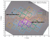 |
Fig. 1 KMTNet fields and cadences. The locations of the events KMT-2017-BLG-0673 and KMT-2019-BLG-0414 are indicated by cross marks. |
3 Light curve analyses
By inspecting the data of the lensing events detected in the peripheral KMTNet fields covered with observational cadences ≥1 h during the 2017–2019 seasons, we found that KMT-2017-BLG-0673 and KMT-2019-BLG-0414 exhibit subtle deviations from the 1L1S models. In Fig. 2, we present the light curves of the two events. From a brief glimpse, the light curves of both events appear to be well described by 1L1S models, which are drawn over the data points. However, a thorough inspection reveal that there exist weak short-term anomalies. We mark the regions of the anomalies for the individual events with grey boxes drawn over the light curves, and the enlarged views of the anomaly regions are shown in Fig. 3 for KMT-2017-BLG-0673 and in Fig. 4 for KMT-2019-BLG-0414.
In the following subsections, we present analyses of both events conducted to explain the observed anomalies in the lensing light curves. As will be discussed, the anomalies are well described by a binary-lens (2L1S) model, in which the mass ratio between the lens components (M1 and M2) is very small.
The 2L1S modeling procedure commonly applied to both events are as follows. In the modeling of each event, we search for a lensing solution, which represents a set of lensing parameters describing the observed lensing light curve. Under the approximation that the relative lens-source motion is rectilinear, a 2L1S event light curve is described by 7 basic parameters. The first three of these parameters (t0, u0, tE) characterize the encounter between the lens and source, and the individual parameters denote the time of the closest lens-source approach, the separation at that time (impact parameter) normalized to the angular Einstein radius θE, and the event time scale, respectively. The event time scale is defined as the time for the source to cross the angular Einstein radius, that is, tE = θE/μ, where μ represents the relative lens-source proper motion. The next three parameters (s, q, α) define the binary lens, and the first two parameters represent the projected separation (scaled to θE) and mass ratio between M1 and M2, respectively, and the third parameter indicates the source trajectory angle defined as the angle between the relative source motion and the binary axis of the lens. The last parameter ρ (normalized source radius), which is defined as the ratio of the angular source radius θ* to θE, characterizes the deformation of a lensing light curve by finite-source effects, which occur during the crossing of a source over the caustic formed by a binary lens.
The searches for the best-fit lensing parameters were carried out in two steps. In the first step, we divided the lensing parameters into two groups, and the binary parameters (s, q) in the first group were searched for via a grid approach with multiple initial values of α evenly divided in the [0 – 2π] range, and the other parameters were found via a downhill approach using a Markov Chain Monte Carlo (MCMC) algorithm. We then construct χ2 maps on the log s–log q–α planes, and identify local solutions on the χ2 maps. In the second step, we refine the individual local solutions by letting all parameters, including s and q, vary. If the degeneracies among different local solutions are severe, we present multiple solutions, and otherwise we present a single global solution.
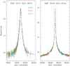 |
Fig. 2 Microlensing light curves of KMT-2017-BLG-0673 and KMT-2019-BLG-0414. The curve drawn over the data points of each light curve is a 1L1S model, and the box indicates the region of the anomaly. The enlarged views of the anomaly regions are shown in Fig. 3 for KMT-2017-BLG-0673 and in Fig. 4 for KMT-2019-BLG-0414. Colors of data points are set to match those of the telescopes marked in the legend. |
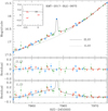 |
Fig. 3 Enlargement of the anomaly region in the lensing light curve of KMT-2017-BLG-0673. The solid and dotted curves drawn over the data points are the 2L1S and 1L1S models, respectively. The residuals from the individual models are shown in the lower two panels. The inset in the top panel shows the lens system configuration, in which the source trajectory (line with an arrow) with respect to the caustic (red figures) is shown. The curve drawn in the bottom panel is the difference between the 2L1S and 1L1S models. |
3.1 KMT-2017-BLG-0673
The anomaly feature of KMT-2017-BLG-0673, shown in Fig. 3, is characterized by a single strong anomaly point at HJD′ ~ 7963.9 (tanom) surrounded by weak positive deviations around tanom during the relatively short time range of 7960 ≲ HJD′ ≲ 7967. The light curve variation at tanom is discontinuous, and this suggests that the anomaly point was produced by the source crossing over a caustic, although the detailed structure of the caustic-crossing feature could not be delineated due to the sparse coverage of the anomaly caused by the low observational cadence of the field.
Considering that the anomaly appears in the peripheral part of the light curve, it is likely that the anomaly was generated by a planetary caustic lying at around the planet-host axis with a separation of uanom ~ s – 1/s from the host (Griest & Safizadeh 1998; Han 2006). In this case, the planet-host separation can be heuristically estimated as
![$s = {1 \over 2}\left[ {{{(u_{{\rm{anom}}}^2 + 4)}^{1/2}} \pm {u_{{\rm{anom}}}}} \right],$](/articles/aa/full_html/2022/10/aa44438-22/aa44438-22-eq4.png) (1)
(1)
where  7964 represents the time of the anomaly. With the values of t0 ~ 797з.3, u0 ~ 0.12, and tE ~ 22 days obtained from the 1L1S modeling conducted by excluding the data points around the anomaly, we find two values of sclose ~ 0.81 and swide ~ 1.24, which correspond to the separations of the close (s < 1.0) and wide (s > 1.0) solutions, respectively.
From the 2L1S modeling, we found a unique solution without any degeneracy. In Table 1, we list the lensing parameters of the solution and the model curve corresponding to the solution is drawn over the data points in Fig. 3. It was found that the 2L1S model improved the fit by ∆χ2 = 584.7 with respect to the 1L1S model. As expected, the anomaly was produced by a low-mass companion with the binary parameters of (s, q) ~ (0.81, 5.6 × 10⁻³). We note that the planet-host separation matches well the value that was heuristically estimated from the location of the anomaly in the lensing light curve.
The lens system configuration, showing the source motion with respect to the caustic, is presented in the inset of the top panel in Fig. 3. It shows that the anomaly was generated by the source passage through one of the two planetary caustics induced by a close planet with s < 1.0. To be noted among the parameters is that the normalized source radius ρ = (7.56 ± 2.32) × 10−3 is measured despite the fact that only a single point covered the caustic. This is possible because the data points lying adjacent to the caustic point provide an extra constraint on the source radius.
A short-term anomaly can also be produced if a source is a binary (Gaudi 1998). We checked this possibility by additionally conducting a binary-source (1L2S) modeling of the light curve. From this modeling, it was found that the 1L2S model yielded a poorer fit to the anomaly than the 2L1S model by ∆χ2 = 30.7, especially in the peripheral region of the anomaly. We, therefore, exclude the 1L2S interpretation of the anomaly. We also checked the feasibility of detecting higher-order effects, including the microlens-parallax effect (Gould 1992) and lens-orbital effect (Batista et al. 2011; Skowron et al. 2011) induced by the orbital motion of Earth and the binary lens, respectively. We found that it was difficult to securely constrain the lensing parameters defining these higher-order effects not only because the event time scale was not long enough but also because the photometry was not sufficiently precise.
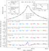 |
Fig. 4 Enlarged view around the anomaly region in the lensing light curve of KMT-2019-BLG-0414. Drawn over the data points are the 1L1S model considering finite-source effects (FSPL), the two 2L1S (solutions 1 and 2) models, and the binary-source model considering xallarap effects (xallarap). The model curves of the two 2L1S models are difficult to be resolved within the line width due to the severe degeneracy between the models. The four bottom panels show the residuals from the individual models. The two left insets in the top panel show the lens-system configurations of the two 2L1S solutions, and the right inset shows the configuration of the xallarap model. The blue and red curves in the bottom panel represent the differences of the 2L1S solutions 1 and 2 from the FSPL model, respectively. |
Lensing parameters of KMT-2017-BLG-0673.
3.2 KMT-2019-BLG-0414
The event KMT-2019-BLG-0414 reached a very high magnification at the peak: Apeak > 200. The anomaly, whose features are shown in Fig. 4, occurred near the peak, and the deviation from the 1L1S model was subtle without any strong signatures, such as would be generated by a caustic crossing. From the inspection of the residual from the 1L1S model, presented in the bottom panel, the feature of the anomaly is characterized by two KMTA points at the peak (HJD′ = 8611.11 and 8611.22) with positive deviations and those around the peak exhibiting slight negative deviations that lasted for about 2.5 days.
From the 2L1S modeling of the light curve, we found 2 sets of planetary solutions with source trajectory angles of α ~ 3.00 (in radian) and ~0.78. We refer to the solutions as 2L1S “solution 1” and “solution 2”, respectively. For each solution, we identified a pair of solutions resulting from the close-wide degeneracy (Griest & Safizadeh 1998; Dominik 1999), and thus there are 4 solutions in total. Regardless of the solution, the estimated mass ratios between the lens components are in the range of [3.3–4.7] × 10−3, indicating that the companion to the lens is a planet. The fit improvement of the 2L1S models with respect to a 1L1S model conducted with the consideration of finite-source effects is ∆χ2 = 90.8, indicating that the planetary signal is securely detected.
In Table 2, we list the lensing parameters of the 4 degenerate planetary 2L1S solutions along with the χ2 values of the fits. The degeneracies among the solutions are very severe with ∆χ2 < 0.2. In Fig. 4, we present the model curves and residuals of solutions 1 and 2. The lens system configurations of the solutions 1 and 2 are shown in the two left insets inserted in the top panel of Fig. 4 where the presented configurations are for the close solutions. Despite the large difference in the source trajectory angle, α ~ 3.00 for solutions 1 and ~0.78 for solution 2, the planet parameters, (s, q) ~ (0.35/2.8, 4.7 × 10⁻³) for solution 1 and (0.42/2.7, 3.3 × 10⁻³) for solution 2, are similar to each other, and thus the caustics of both solutions appear to be similar to each other. For both solutions, the anomaly was produced by the source approach close to the central caustic induced by a planetary companion. The two points with positive deviations appeared when the source approached the cusp of the caustic. Although the normalized source radius cannot be measured because the source did not cross the caustic, the modeling yields an upper limit of ρmax ~ 5 × 10⁻³.
We additionally checked the binary-source origin the anomaly. Under the static 1L2S interpretation without the orbital motion of the source, we found that the anomaly could not be explained by the model because the light curve exhibited both positive and negative deviations, while the 1L2S model could produce only positive deviations. However, a negative deviation can be produced by a xallarap effect, in which a faint source companion induces a variation of the primary source motion by the orbital motion (Griest & Hu 1992; Han & Gould 1997). Following the parameterization of Dong et al. (2009), we thus carried out a xallarap modeling by adding 5 extra parameters of (ξE,N, ξE,E, P, ϕ, i) to those of the 1L1S model. Here (ξE,N, ξE,E) are the north and east components of the xallarap vector ξE, P denotes the orbital period, ϕ is the phase angle, and i represents the inclination of the source orbit. From this modeling, we found a xallarap solution that approximately explained the observed anomaly. We list the lensing parameters of the bestfit xallarap solution in Table 2, and present the model curve, its residual, and the lens system configuration in Fig. 4. According to the model, the source is accompanied by a close faint companion inducing a very short orbital period of ~1 day. Although the xallarap fit is not preferred over the 2L1S solutions, the χ2 difference is minor with ∆χ2 ~ 4.2. We, therefore, consider the xallarap solution as a viable interpretation of the event. Had the Einstein radius of the lens system been measured, the minimum mass of the source companion could be constrained by the relation of  to judge the validity of the xallarap solution, but this constraint could not be applied to the lens system because the normalized source radius could not be measured. Here
  denotes the physical Einstein radius projected on the source plane. We note that the model curves of the 2L1S and xallarap solutions differ from each other in the region not covered by data points, indicating that the degeneracy between the solutions could have been resolved if the event had more continuous coverage. In particular, the two models differ by ~0.1 mag during the KMTC observing window centered on HJD′ ~ 8610.75. Unfortunately, KMTC was weathered out on that night.
4 Source stars and Einstein radii
In this section, we characterize the source stars of the events. Characterizing the source star is important not only to fully describe the event but also to measure the Einstein radius, which is related to the lensing parameter of the normalized source radius by
 (2)
(2)
where the angular source radius can be deduced from the source type. See below for the detailed procedure of the θ* estimation. Measurement of the Einstein radius is important because it is related to the mass M and distance to the lens DL as θE = (κMπrel)1/2, and thus θE can provide an extra constraint on the mass and distance to the lens in addition to the basic observable of the event time scale. Here κ ≡ 4G/c2 AU ≃ 8.14 mas  and πrel represents the relative lens-source parallax, that is,
  , where DS is the distance to the source. We specified the source stars of the events by measuring their color and brightness. In order to estimate the extinction- and reddening-corrected (de-reddened) color and magnitude of the source, (V − I, I)S,0, from the instrumental values, (V − I, I)S, we applied the Yoo et al. (2004) routine. In this routine, the centroid of the red giant clump (RGC) in the color-magnitude diagram (CMD) with its known de-reddened color and magnitude (Bensby et al. 2013; Nataf et al. 2013) was used as a reference for the calibration of the source color and brightness.
Figure 5 shows the CMDs of stars lying in the neighborhood of the source stars of the two events constructed with the photometry data processed using the pyDIA code (Albrow 2017). In each CMD, we mark the positions of the source and RGC cen-troid by a blue dot and a red dot, respectively. Also marked is the position of a blend, which is marked by a green dot, indicating that the blended fluxes of both events are dominated by bright disk stars. We will discuss the nature the blend in the following section. For the estimation of the source position in the CMD, we measured the I- and V-band magnitudes of the source by regressing the data of the individual passbands processed using the pyDIA photometry code with the variation of the lensing magnification. By measuring the offsets in color and magnitude between the source and RGC centroid in the CMD, ∆(V − I, I) = [(V − I, I)S – (V − I, I)RGC], then the de-reddened color and magnitude of the source were estimated as
 (3)
(3)
In Table 3, we list the values of (V − I, I)S, (V − I, I)RGC, (V − I, I)RGC,0, and (V − I, I)0,S for the two lensing events. According to the measured color and magnitude, it was found that the source of KMT-2017-BLG-0673 was a K-type giant and the source of KMT-2019-BLG-0414 was a G-type main-sequence star.
We estimated the source radii of the events by first converting V − I into V − K using the color-color relation of Bessell & Brett (1988), and then derived θ* from the (V − K, V)−θ* relation of Kervella et al. (2004). The estimated angular radii of the source stars are
 (4)
(4)
From the relation in Eq. (2), it is estimated that the angular Einstein radii of the two events are
 (5)
(5)
With the values of the event time scales, the relative lens-source proper motions, μ = θE/tE, are estimated as
 (6)
(6)
For KMT-2019-BLG-0414, we present the lower limits of θE and μ because only an upper limit on ρ is obtained for this event.
Lensing parameters of KMT-2019-BLG-0414.
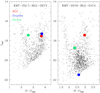 |
Fig. 5 Source locations with respect to the centroids of red giant clump (RGC) in the instrumental color-magnitude diagrams of stars lying in the neighborhood of the source of KMT-2017-BLG-0673 and KMT-2019-BLG-0414 constructed using the pyDIA photometry of KMTC data set. Also marked are the positions of the blend. |
Source properties.
5 Physical lens parameters
The physical parameters of the lens mass and distance are constrained by the lensing observables of tE, θE, and πE, which are related to the physical parameters. The basic parameter of the event time scale was securely measured for both events, the Einstein radius was measured for KMT-2017-BLG-0673, while only a lower limit was obtained for KMT-2019-BLG-0414. However, the microlens parallax could not be measured for either event. Although the partial measurements of the lensing observables make it difficult to uniquely determine M and DL from the relations (Gould 2000)
 (7)
(7)
it is still possible to constrain the physical parameters with the measured observables of the individual events from a Bayesian analysis.
In the Bayesian analysis, we first produced a large number (107) of lensing events by conducting a Monte Carlo simulation based on a Galactic model. The Galactic model defines the matter density, motion, and mass function of Galactic objects. From the physical parameters of the simulated events, we computed the lensing observables of tE,i = DLθE/υ⊥ and θE,i = (κMπrel)1/2. Here υ⊥ represents the transverse speed between the lens and source. We then constructed Bayesian posteriors of the lens mass and distance with a weight assigned to each simulated event computed by wi = exp(−χ2/2), where χ2 = (tE,i − tE)2/σ(tE)2 + (θE,i − θE)2/σ(θE)2, σ(tE) and σ(θE) represent the uncertainties of tE and θE estimated from the modeling, respectively. In the simulation of lensing events, we used the Jung et al. (2021) Galactic model.
In Figs. 6 and 7, we present the posteriors of the host mass and distance to the planetary systems, respectively. For each distribution, the solid vertical line denotes the median value, and the two dotted vertical lines represent the 1er range estimated as 16% and 84% of the distribution. We separately mark posterior distributions of the disk and bulge lens populations with blue and red curves, respectively. In Table 4, we summarize the estimated masses of the host (Mh) and planet (Mp), distances, and projected planet-host separations (a⊥ = sDLθE) for the two planetary systems. For KMT-2019-BLG-0414, we present four sets of parameters corresponding to the four degenerate solutions. We note that the primary mass and distance of KMT-2019-BLG-0414L estimated from the degenerate solutions are alike regardless of the solution because the constraint given by the lower limit of θE is very weak and the other constraint of the event time scales of the degenerate solutions are nearly identical.
It is found that the two planetary systems are very similar to each other in many aspects. First, both systems have planets heavier than the Jupiter of the Solar system with masses Mp ~ 3.7 MJ and ~[2.0−4.5] MJ for KMT-2017-BLG-0673L and KMT-2019-BLG-0414L, respectively. Second, the masses of the planet hosts, Mh ~ 0.6 M⊙ and −0.7 M⊙ for the individual lenses, are also similar to each other. Third, the distances to the systems, DL ~ 5.1 kpc and ~4.4 kpc, indicate that both planetary systems are likely to be in the disk. According to the Bayesian estimation, the probability for the planetary system to be in the disk is ~63% for KMT-2017-BLG-0673L and ~73% for KMT-2019-BLG-0414L.
Prompted by the facts that the lenses of both events are likely to be in the disk and the blended fluxes come from disk stars, we inspected the possibility of the lenses of the events to be the main sources of the blended flux. For this inspection, we examined the reference images taken before the lensing magnification and the difference image taken during the lensing magnification. For KMT-2017-BLG-0673, there exists a star even brighter than the source of a bulge giant at a location with a separation of ~2.2 arcsec from the source, and this degrades the photometry and astrometry of the event together with the high extinction, AI ~ 3.1 mag, toward the field. Nevertheless, we identified a blend lying at a separation of ~0.65 arcsec from the source with a brightness corresponding to the blend. This indicates that the lens is not the main source of the blended flux. For KMT-2019-BLG-0414, the astrometric offset between the centroid of baseline object measured on the reference image, θref = [(fs/fb)θs + θb]/(fs/fb + 1), and the source position measured on the difference image, θs, is ∆θ = |θref − θs| = (79.2 ± 59.2) mas. Here fs and fb represent the flux values of the source and blend, respectively. In the case of KMT-2019-BLG-0414, fb ≫ fs, and thus the centroid shift can be approximated as Δθ ~ |θb − θs|. Considering that the measured astrometric offset is only 1.3 times greater than the uncertainty, it is difficult to firmly exclude the possibility that the lens is the major source of blended light based on the argument of the measurement uncertainty.
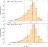 |
Fig. 6 Bayesian posteriors of the host mass for the planetary systems KMT-2017-BLG-0673L (upper panel) and KMT-2019-BLG-0414L (lower panel). The vertical line in each panel represents the median value and the two dotted vertical lines indicate the 1σ range of the distribution. The curves drawn in blue and red represent the contributions of the disk and bulge lens populations, respectively. |
Physical lens parameters
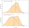 |
Fig. 7 Bayesian posteriors of the distance to the planetary system. Notations are same as those in Fig. 6. |
6 Resolution of KMT-2019-BLG-0414 degeneracy
In this section, we discuss the possibility of resolving the degeneracy between the 2L1S and xallarap solutions of KMT-2019-BLG-0414 by means of AO observations on 30 m class telescopes, which may see first light in about 2030. We give a brief synopsis of the decision tree governing these observations.
In the 2L1S model, ρ < 0.005 at 3σ confidence, which implies, μ > 0.7 mas yr−1 (see Eq. (6)). If μ is really at the threshold of this limit, then several decades would be required to separately resolve the lens and source. However, typical lens-source relative proper motions are substantially higher than this, and therefore, most likely, 30 m-class AO imaging in 2030 will resolve them. This will yield a heliocentric proper motion measurement. One must be careful to correct from heliocentric to geocentric proper motion using
 (8)
(8)
where v⊕,⊥(N, E) = (−0.7, +21.6) km s−1 is the projected velocity of Earth at the peak of the event. However, we ignore this correction in the following simplified treatment. Because tE ≃ yr/5 is well measured in both models, such a proper motion measurement will immediately yield a determination of the Einstein radius: θE =≃ 0.6 mas (μ/3 mas yr−1).
Within the context of the xallarap model, this will yield the semi-major axis of the orbit of the primary, i.e., aprimary = ξθEDS = 1.25 R⊙ (μ/3 mas yr−1), where we have assumed a source distance of DS = 8 kpc. Combined with the period measurement P = 0.9 day, a source-mass estimate of MS = 1 M⊙ and Kepler's Third Law, this will yield the mass of the source companion. For example, for μ = 3 mas yr−1, Mcompanion ~ 0.4 M⊙ (which would account for its lack of photometric signature). However, if μ were measured to be sufficiently large, this might imply photometric signatures from a luminous orbiting companion and (or) eclipses, which might rule out the xallarap scenario.
Assuming that xallarap solutions survive this test, there remains a radial-velocity (RV) test of the xallarap hypothesis. The amplitude of the RV signature would be υ sin i = 2π(aprimary/P) sin i = 70 km s−1 (μ/3 mas yr−1) sin i. The source is IS ~ 21.5 (KS ~ 18.0), so RV signatures of amplitude ≪1 km s−1 should be detectable with 30 m-class AO spectroscopy. If these signatures are not detected, then the xallarap model would become highly implausible because it would require an almost perfectly face-on orbit. For completeness, we note that Gaia DR3 reports a parallax and proper motion for the baseline object of πbase = (1.1 ± 0.4) mas and μbase(E, N) = (−0.4 ± 0.4, −2.3 ± 0.3) mas yr−1. As shown in Fig. 5, the baseline object is dominated by the blend. While the parallax error is large, the low proper motion is also consistent with the blend being a nearby object. This object is most likely dominated by the host or a companion to the host. By the time 30 m-class AO is available, the parallax error will likely be reduced by a factor ~1.7, so Gaia astrometry may substantially aid the interpretation of the AO images.
7 Summary
We presented analyses of two microlensing events KMT-2017-BLG-0673 and KMT-2019-BLG-0414, for which the presence of planets in the lenses were found from the inspection of the microlensing data collected by the KMTNet survey during the 2017-2019 seasons in the peripheral Galactic bulge fields. The planetary signal of KMT-2017-BLG-0673 had been previously missed because of the relatively sparse coverage of the event, and the signal of KMT-2019-BLG-0414 had not been identified due to the weakness of the signal caused by its non-caustic-crossing nature. The detections of the planets indicate the need for thorough investigations of non-prime-field lensing events for the complete census of microlensing planet samples.
For KMT-2017-BLG-0673, we identified a unique planetary solution with lensing parameter of (s, q) ~ (0.81, 5.6 × 10⁻³). It was found that the planetary signal was generated by the source passage through one of the two tiny planetary caustics induced by a planet lying inside the Einstein ring of the planetary system.
For KMT-2019-BLG-0414, on the other hand, we identified two pairs of solutions, for each of which there were two solutions caused by the close-wide degeneracy. Despite the fact that the incidence angles of the two sets of solutions differed from each other, the planet parameters of the projected planet-host separations and mass ratios were similar to each other. Although slightly less favored, the anomaly could also be explained by a model, in which a single lens mass magnified a rapidly orbiting binary source with a faint companion. In Sect. 6, we discussed how the planet/xallarap degeneracy might one day be resolved by AO observations on 30 m class telescopes. Pending such resolution, KMT-2019-BLG-0414Lb should not be included in catalogs of “known planets”.
From the physical parameters estimated by conducting Bayesian analyses based on the observables of the events, it was found that the two planetary systems were similar to each other in many aspects. For both planetary systems, the hosts of the planets are stars with masses lower than the Sun, and they host planets heavier than the Jupiter of the Solar system. Furthermore, both planetary systems reside in the disk of the Galaxy.
Acknowledgements
Work by C.H. was supported by the grants of National Research Foundation of Korea (2020R1A4A2002885 and 2019R1A2C2085965). This work was financially supported by the Research Year of Chungbuk National University in 2021. This research has made use of the KMTNet system operated by the Korea Astronomy and Space Science Institute (KASI) and the data were obtained at three host sites of CTIO in Chile, SAAO in South Africa, and SSO in Australia. J.C.Y. acknowledges support from NSF Grant No. AST-2108414. W.Z. and H.Y. acknowledge the support by the National Science Foundation of China (Grant No. 12133005).
References
- Albrow, M. 2017, MichaelDAlbrow/pyDIA: Initial Release on Github, Versionv1.0.0, Zenodo, https://doi.org/10.5281/zenodo.268049 [Google Scholar]
- Albrow, M., Horne, K., Bramich, D.M., et al. 2009, MNRAS, 397, 2099 [NASA ADS] [CrossRef] [Google Scholar]
- Batista, V., Gould, A., Dieters, S., et al. 2011, A&A, 529, A102 [NASA ADS] [CrossRef] [EDP Sciences] [Google Scholar]
- Bensby, T., Yee, J.C., Feltzing, S., et al. 2013, A&A, 549, A147 [NASA ADS] [CrossRef] [EDP Sciences] [Google Scholar]
- Bessell, M.S., & Brett, J.M. 1988, PASP, 100, 1134 [NASA ADS] [CrossRef] [Google Scholar]
- Bond, I.A., Abe, F., Dodd, R.J., et al. 2001, MNRAS, 327, 868 [NASA ADS] [CrossRef] [Google Scholar]
- Dominik, M. 1999, A&A, 349, 108 [NASA ADS] [Google Scholar]
- Dong, S., Gould, A., Udalski, A., et al. 2009, ApJ, 695, 970 [NASA ADS] [CrossRef] [Google Scholar]
- Gaudi, B.S. 1998, ApJ, 506, 533 [NASA ADS] [CrossRef] [Google Scholar]
- Gaudi, B.S. 2012, ARA&A, 50, 411 [NASA ADS] [CrossRef] [Google Scholar]
- Gould, A. 1992, ApJ, 392, 442 [Google Scholar]
- Gould, A. 2000, ApJ, 542, 785 [NASA ADS] [CrossRef] [Google Scholar]
- Gould, A., & Loeb, A. 1992, ApJ, 396, 104 [Google Scholar]
- Gould, A., Han, C., Zang, W., et al. 2022, A&A, 664, A13 [NASA ADS] [CrossRef] [EDP Sciences] [Google Scholar]
- Griest, K., & Hu, W., 1992, ApJ, 397, 362 [Google Scholar]
- Griest, K., & Safizadeh, N. 1998, ApJ, 500, 37 [Google Scholar]
- Han, C. 2006, ApJ, 638, 1080 [Google Scholar]
- Han, C., & Gould, A. 1997, ApJ, 480, 196 [NASA ADS] [CrossRef] [Google Scholar]
- Han, C., Udalski, A., Kim, D., et al. 2020, A&A, 642, A110 [EDP Sciences] [Google Scholar]
- Han, C., Udalski, A., Kim, D., et al. 2021a, A&A, 650, A89 [NASA ADS] [CrossRef] [EDP Sciences] [Google Scholar]
- Han, C., Udalski, A., Kim, D., et al. 2021b, A&A, 655, A21 [NASA ADS] [CrossRef] [EDP Sciences] [Google Scholar]
- Han, C., Gould, A., Albrow, M.D., et al. 2022, A&A, 658, A62 [NASA ADS] [CrossRef] [EDP Sciences] [Google Scholar]
- Hwang, K.-H., Zang, W., Gould, A., et al. 2022, AJ, 163, 43 [NASA ADS] [CrossRef] [Google Scholar]
- Jung, Y.K., Gould, A., Udalski, A., et al. 2020a, AJ, 160, 148 [NASA ADS] [CrossRef] [Google Scholar]
- Jung, Y.K., Udalski, A., Zang, W., et al. 2020b, AJ, 160, 255 [NASA ADS] [CrossRef] [Google Scholar]
- Jung, Y.K., Han, C., Udalski, A., et al. 2021, AJ, 161, 293 [NASA ADS] [CrossRef] [Google Scholar]
- Jung, Y.K., Zang, W., Han, C., et al. 2022, AJ, submitted [arXiv:2206.11409] [Google Scholar]
- Kervella, P., Thévenin, F., Di Folco, E., & Ségransan, D. 2004, A&A, 426, 29 [Google Scholar]
- Kim, S.-L., Lee, C.-U., Park, B.-G., et al. 2016, JKAS, 49, 37 [Google Scholar]
- Kim, D.-J., Kim, H.-W., Hwang, K.-H., et al. 2018a, AJ, 155, 76 [Google Scholar]
- Kim, H.-W., Hwang, K.-H., Shvartzvald, Y., et al. 2018b, ArXiv eprints [arXiv:1806.07545] [Google Scholar]
- Laughlin, G., Bodenheimer, P., & Adams, F.C. 2004, ApJ, 612, L73 [NASA ADS] [CrossRef] [Google Scholar]
- Nataf, D.M., Gould, A., Fouqué, P., et al. 2013, ApJ, 769, 88 [NASA ADS] [CrossRef] [Google Scholar]
- Skowron, J., Udalski, A., Gould, A., et al. 2011, ApJ, 738, 87 [Google Scholar]
- Udalski, A., Szymanski, M.K., & Szymanski, G. 2015, Acta Astron., 65, 1 [NASA ADS] [Google Scholar]
- Wang, H., Zang, W., Zhu, W., et al. 2022, MNRAS, 510, 1778 [Google Scholar]
- Yee, J.C., Shvartzvald, Y., Gal-Yam, A., et al. 2012, ApJ, 755, 102 [NASA ADS] [CrossRef] [Google Scholar]
- Yoo, J., DePoy, D.L., Gal-Yam, A., et al. 2004, ApJ, 603, 139 [NASA ADS] [CrossRef] [Google Scholar]
- Zang, W., Hwang, K.-H., Udalski, A., et al. 2021, AJ, 162, 163 [NASA ADS] [CrossRef] [Google Scholar]
- Zang, W., Yang, H., Han, C., et al. 2022, MNRAS, 515, 928 [NASA ADS] [CrossRef] [Google Scholar]
All Tables
All Figures
|
Fig. 1 KMTNet fields and cadences. The locations of the events KMT-2017-BLG-0673 and KMT-2019-BLG-0414 are indicated by cross marks. |
| In the text | |
|
Fig. 2 Microlensing light curves of KMT-2017-BLG-0673 and KMT-2019-BLG-0414. The curve drawn over the data points of each light curve is a 1L1S model, and the box indicates the region of the anomaly. The enlarged views of the anomaly regions are shown in Fig. 3 for KMT-2017-BLG-0673 and in Fig. 4 for KMT-2019-BLG-0414. Colors of data points are set to match those of the telescopes marked in the legend. |
| In the text | |
|
Fig. 3 Enlargement of the anomaly region in the lensing light curve of KMT-2017-BLG-0673. The solid and dotted curves drawn over the data points are the 2L1S and 1L1S models, respectively. The residuals from the individual models are shown in the lower two panels. The inset in the top panel shows the lens system configuration, in which the source trajectory (line with an arrow) with respect to the caustic (red figures) is shown. The curve drawn in the bottom panel is the difference between the 2L1S and 1L1S models. |
| In the text | |
|
Fig. 4 Enlarged view around the anomaly region in the lensing light curve of KMT-2019-BLG-0414. Drawn over the data points are the 1L1S model considering finite-source effects (FSPL), the two 2L1S (solutions 1 and 2) models, and the binary-source model considering xallarap effects (xallarap). The model curves of the two 2L1S models are difficult to be resolved within the line width due to the severe degeneracy between the models. The four bottom panels show the residuals from the individual models. The two left insets in the top panel show the lens-system configurations of the two 2L1S solutions, and the right inset shows the configuration of the xallarap model. The blue and red curves in the bottom panel represent the differences of the 2L1S solutions 1 and 2 from the FSPL model, respectively. |
| In the text | |
|
Fig. 5 Source locations with respect to the centroids of red giant clump (RGC) in the instrumental color-magnitude diagrams of stars lying in the neighborhood of the source of KMT-2017-BLG-0673 and KMT-2019-BLG-0414 constructed using the pyDIA photometry of KMTC data set. Also marked are the positions of the blend. |
| In the text | |
|
Fig. 6 Bayesian posteriors of the host mass for the planetary systems KMT-2017-BLG-0673L (upper panel) and KMT-2019-BLG-0414L (lower panel). The vertical line in each panel represents the median value and the two dotted vertical lines indicate the 1σ range of the distribution. The curves drawn in blue and red represent the contributions of the disk and bulge lens populations, respectively. |
| In the text | |
|
Fig. 7 Bayesian posteriors of the distance to the planetary system. Notations are same as those in Fig. 6. |
| In the text | |
Current usage metrics show cumulative count of Article Views (full-text article views including HTML views, PDF and ePub downloads, according to the available data) and Abstracts Views on Vision4Press platform.
Data correspond to usage on the plateform after 2015. The current usage metrics is available 48-96 hours after online publication and is updated daily on week days.
Initial download of the metrics may take a while.