| Issue |
A&A
Volume 692, December 2024
|
|
|---|---|---|
| Article Number | A95 | |
| Number of page(s) | 25 | |
| Section | Extragalactic astronomy | |
| DOI | https://doi.org/10.1051/0004-6361/202244401 | |
| Published online | 03 December 2024 | |
Optical and near-infrared photometry of 94 type II supernovae from the Carnegie Supernova Project
1
European Southern Observatory, Alonso de Córdova 3107, Casilla 19, Santiago, Chile
2
Carnegie Observatories, Las Campanas Observatory, Casilla 601, La Serena, Chile
3
Department of Physics and Astronomy, Aarhus University, Ny Munkegade 120, DK-8000 Aarhus C, Denmark
4
“Fundación Chilena de Astronomía”, El Vergel 2252 #1501, Santiago, Chile
5
George P. and Cynthia Woods Mitchell Institute for Fundamental Physics and Astronomy, Department of Physics and Astronomy, Texas A&M University, College Station, TX 77843, USA
6
Centre for Astrophysics and Gravitation, Instituto Superior Técnico, University of Lisbon, Av. Rovisco Pais 1, 1049-001 Lisbon, Portugal
7
Institut d’Estudis Espacials de Catalunya (IEEC), Edifici RDIT, Campus UPC, 08860 Castelldefels (Barcelona), Spain
8
Institute of Space Sciences (ICE, CSIC), Campus UAB, Carrer de Can Magrans, s/n, E-08193 Barcelona, Spain
9
The Observatories of the Carnegie Institution for Science, 813 Santa Barbara St., Pasadena, CA 91101, USA
10
Department of Physics, Florida State University, Tallahassee, FL 32306, USA
11
Centro de Astronomía (CITEVA), Universidad de Antofagasta, Av. Angamos 601, Antofagasta, Chile
12
Institute for Astronomy, University of Hawaii, 2680 Woodlawn Drive, Honolulu, HI 96822, USA
13
Department of Physics, Yale University, 217 Prospect Street, New Haven, CT 06511, USA
14
Planetary Science Institute, 1700 East Fort Lowell Road, Suite 106, Tucson, AZ 85719-2395, USA
15
Hamburger Sternwarte, Gojenbergsweg 112, 21029 Hamburg, Germany
16
Homer L. Dodge Department of Physics and Astronomy, University of Oklahoma, Rm 100 440 W. Brooks, Norman, OK 73019-2061, USA
17
Facultad de Ciencias Astronomicas y Geofisicas, Universidad Nacional de La Plata, Instituto de Astrofisica de La Plata (IALP), CONICET, Paseo del Bosque SN, B1900FWA La Plata, Argentina
18
Kavli Institute for the Physics and Mathematics of the Universe (WPI), The University of Tokyo, 5-1-5 Kashiwanoha, Kashiwa, Chiba 277-8583, Japan
19
Observatoire du Mont-Mégantic, Département de Physique, Université de Montréal, Montréal, Canada
20
Department of Astronomy, University of California, Berkeley, CA 94720-3411, USA
21
Data and Artificial Intelligence Initiative (D&IA), University of Chile, Santiago, Chile
22
Millennium Institute of Astrophysics (MAS), Nuncio Monseñor Sótero Sanz, Providencia, Santiago, Chile
23
Center for Mathematical Modeling, University of Chile, AFB170001 Santiago, Chile
24
Departamento de Astronomía, Universidad de Chile, Casilla 36D, Santiago, Chile
25
Institut d’Estudis Espacials de Catalunya (IEEC), Gran Capità, 2-4, Edifici Nexus, Desp. 201, E-08034 Barcelona, Spain
26
DARK, Niels Bohr Institute, University of Copenhagen, Jagtvej 128, 2200 Copenhagen, Denmark
27
The Oskar Klein Centre, Department of Physics, Stockholm University, SE-106 91 Stockholm, Sweden
28
Infrared Processing and Analysis Center, Caltech/Jet Propulsion Laboratory, Pasadena, CA 91125, USA
29
Lawrence Berkeley National Laboratory, Department of Physics, 1 Cyclotron Road, Berkeley, CA 94720, USA
30
The Oskar Klein Centre, Department of Astronomy, Stockholm University, AlbaNova, SE-10691 Stockholm, Sweden
31
School of Mathematical and Physical Sciences, Macquarie University, Sydney, NSW 2109, Australia
32
Astrophysics and Space Technologies Research Centre, Macquarie University, Sydney, NSW 2109, Australia
33
Cerro Tololo Inter-American Observatory/NSFs NOIRLab, Casilla 603, La Serena, Chile
34
NOIRLab, Avda Juan Cisternas 1500, La Serena, Chile
35
Gemini Observatory/NSF’s NOIRLab, Casilla 603, La Serena, Chile
36
Department of Physics and Astronomy, University of South Carolina, Columbia, SC, 29208, USA
⋆ Corresponding author; janderso@eso.org
Received:
1
July
2022
Accepted:
30
August
2024
Context. Type II supernovae (SNe II) mark the endpoint in the lives of hydrogen-rich massive stars. Their large explosion energies and luminosities allow us to measure distances, metallicities, and star formation rates into the distant Universe. To fully exploit their use in answering different astrophysical problems, high-quality low-redshift data sets are required. Such samples are vital to understand the physics of SNe II, but also to serve as calibrators for distinct – and often lower-quality – samples.
Aims. We present uBgVri optical and YJH near-infrared (NIR) photometry for 94 low-redshift SNe II observed by the Carnegie Supernova Project (CSP). A total of 9817 optical and 1872 NIR photometric data points are released, leading to a sample of high-quality SN II light curves during the first ∼150 days post explosion on a well-calibrated photometric system.
Methods. The sample is presented and its properties are analysed and discussed through comparison to literature events. We also focus on individual SNe II as examples of classically defined subtypes and outlier objects. Making a cut in the plateau decline rate of our sample (s2), a new subsample of fast-declining SNe II is presented.
Results. The sample has a median redshift of 0.015, with the nearest event at 0.001 and the most distant at 0.07. At optical wavelengths (V), the sample has a median cadence of 4.7 days over the course of a median coverage of 80 days. In the NIR (J), the median cadence is 7.2 days over the course of 59 days. The fast-declining subsample is more luminous than the full sample and shows shorter plateau phases. Of the non-standard SNe II highlighted, SN 2009A particularly stands out with a steeply declining then rising light curve, together with what appears to be two superimposed P-Cygni profiles of Hα in its spectra. We outline the significant utility of these data, and finally provide an outlook of future SN II science.
Key words: techniques: photometric / catalogs / supernovae: general
© The Authors 2024
 Open Access article, published by EDP Sciences, under the terms of the Creative Commons Attribution License (https://creativecommons.org/licenses/by/4.0), which permits unrestricted use, distribution, and reproduction in any medium, provided the original work is properly cited.
This article is published in open access under the Subscribe to Open model. Subscribe to A&A to support open access publication.
1. Introduction
Supernovae displaying strong, long-lasting, and broad hydrogen features in their visual-wavelength spectra are known as type II supernovae (SNe II)1. These events are the most common SNe in the local Universe (Li et al. 2011), and are believed to result from the core collapse of massive stars (> 8–10 M⊙) that arrive to their deathbeds with a significant fraction of their hydrogen envelopes intact. The display of prevalent Balmer spectral lines defines their type II designation (Minkowski 1941), as opposed to type I events that do not show hydrogen features. This presence of hydrogen, together with the slowly declining (plateau) nature of their light curves, was the basis for early conclusions of red-supergiant (RSG) progenitors, that is, explosions of massive stars with extended envelopes (e.g. Grassberg et al. 1971; Chevalier 1976; Falk & Arnett 1977). Such conclusions received significant support through the almost exclusively star-forming nature of the host galaxies of SNe II (Maza & van den Bergh 1976, see, e.g. Hakobyan et al. 2012 for a modern analysis), implying massive star progenitors.
The high relative rates of SNe II together with their intrinsic brightness mean that they are important objects for our overall understanding of the Universe. SNe II contribute to the chemical enrichment of the interstellar medium, and their energetics are thought to play a role in both galaxy evolution and in triggering subsequent episodes of star formation (SF). In addition, given their luminosities, rates, and direct relationship to massive SF, SNe II allow us to measure key astrophysical parameters across a large volume of the Universe. It is therefore important that we expand our knowledge of these explosive events, both to understand the progenitors and explosion mechanisms as worthy knowledge in itself, and to bolster confidence in our use of SNe II to understand the Universe at large.
The direct detection of progenitor stars on pre-explosion imaging (e.g. Van Dyk et al. 2003; Smartt et al. 2004; see Smartt 2015 for a review), confirmed earlier modelling conclusions that most SNe II are the result of RSG star explosions. While the number remains low, the statistical significance of the high-quality direct detections constrains the zero age main sequence (ZAMS) mass range to be between 8.5 and 18 M⊙ (Smartt 2015). This led to claims of a ‘RSG problem’ (Smartt et al. 2009), given that > 18 M⊙ RSG stars are known to exist in the local Universe (e.g. Levesque et al. 2005), and are expected to explode as SNe II. While a number of explanations for this ‘problem’ have been discussed (Kochanek et al. 2008; Yoon & Cantiello 2010; Walmswell & Eldridge 2012; Smartt 2015; Davies & Beasor 2018; Limongi & Chieffi 2018), the statistical significance has also been questioned (Davies & Beasor 2020). In any case, there is now a general consensus that the majority of SNe II are the result of RSG explosions. However, direct mapping of progenitor properties such as ZAMS mass, metallicity, rotation, and binarity to the observed diversity of SN II transient features is still lacking.
SNe II were historically separated into type IIP and IIL (Barbon et al. 1979). The former plateau events show an almost constant luminosity lasting several months, while the latter ‘linear’ explosions decline significantly faster. However, recent large-sample analyses have argued against distinct classes (e.g. Anderson et al. 2014a, A14 henceforth). We therefore refrain from making such subjective separations for the majority of this paper, only doing so when comparison to the literature is required. Another three further subclasses of SNe II exist in the spectroscopically defined types IIn and IIb (see Filippenko 1997 for a review), and those events showing similar light curves to the iconic SN 1987A. These events are somewhat distinct from the ‘normal’ SN II class we concentrate on here, and probably arise from somewhat different progenitors. They are therefore not discussed in any further detail. However, updated photometry for Carnegie Supernova Project-I SNe IIn and SN 1987A-like events is released here – readers are referred to the Appendix for more details. (For an overview of core-collapse and hydrogen-rich SN observations and interpretations, the reader is referred to Arcavi 2017; Modjaz et al. 2019).
Until recently, the majority of SN II studies concentrated on individual events (see e.g. Hamuy et al. 2001; Leonard et al. 2002b; Pastorello et al. 2006), or on specific correlations for their use as distance indicators (e.g. Hamuy & Pinto 2002). However, to understand the full diversity of events, and hence the full diversity of progenitor and explosion properties, large samples are required. A14 presented a characterisation of the V-band light curves of 117 SNe II (a combination of the events from the current data release and those from Galbany et al. 2016). A range of observational parameters was defined and used to investigate correlations between SN II luminosity, decline rates, and light-curve time scales. While some intriguing trends were observed, that work also highlighted the huge diversity of the SN II class, with significant variance in both SN brightness and overall light-curve morphology. A number of other studies have arrived at similar conclusions (Pskovskii 1967; Young & Branch 1989; Patat et al. 1994; Richardson et al. 2002; Arcavi et al. 2012; Bersten 2013; Faran et al. 2014a,b; González-Gaitán et al. 2015; Sanders et al. 2015; Valenti et al. 2016; Rubin et al. 2016; Rubin & Gal-Yam 2016; Galbany et al. 2016; de Jaeger et al. 2019). Large diversity is also observed in the spectral properties of SNe II (see, e.g. Pastorello et al. 2005; Inserra et al. 2013; Anderson et al. 2014b; Spiro et al. 2014; Gutiérrez et al. 2014; Faran et al. 2014a,b; Gutiérrez et al. 2017a,b; de Jaeger et al. 2019; Davis et al. 2019), where trends are also observed between spectroscopic and photometric parameters. Attempting to understand this diversity aids in furthering our understanding of progenitor properties and explosion characteristics. Understanding SN II diversity is also vital for the current and future use of SNe II as astrophysical probes.
A number of methods have been developed to enable the use of SNe II as distance indicators. These include the Expanding Photosphere Method (EPM, Kirshner & Kwan 1974; Schmidt et al. 1994; Hamuy 2001), the Standard Candle Method (SCM, Hamuy & Pinto 2002), the Spectral-fitting Expanding Atmosphere Method (SEAM, Baron et al. 2004; Dessart et al. 2008), the Photospheric Magnitude Method (PMM, Rodríguez et al. 2014, 2019), and most recently the Photometric Colour Method (PCM, de Jaeger et al. 2015). Recent examples of these methods applied to samples of SNe II located at cosmologically interesting distances are presented by Gall et al. (2016, 2018), de Jaeger et al. (2017a,b), and de Jaeger et al. (2020).
It has also been shown, first through modelling (Dessart et al. 2013, 2014) and later through observations (Anderson et al. 2016), that SNe II can be used to measure metallicities. Being able to measure both distances and metallicities, SNe II show great potential to probe such quantities out to cosmological distances, hence affording independent constraints on the evolution of the Universe. This can only be achieved if well observed, nearby samples exist – against which data can be compared and calibrated. The purpose of the current paper is to release such a data set for widespread use.
Many individual photometric and spectral data sets of SNe II have been published. Recent years have also seen the publication of SN II data samples. Faran et al. (2014a,b), and later de Jaeger et al. (2019) released optical photometric and spectral data for a total of 90 SNe II obtained by the Lick Observatory Supernova Search (LOSS; Filippenko et al. 2001) programme. Galbany et al. (2016) published optical photometry for 51 events from a range of SN II follow-up surveys, while Hicken et al. (2017) published optical and near-infrared (NIR) light curves together with optical spectra for another 39 SNe II from the Center for Astrophysics group. In the current paper, we present optical and NIR photometry of 74 SNe II2 obtained by the Carnegie Supernova Project-I (hereafter CSP-I, Hamuy et al. 2006), together with data from an additional 20 objects observed by the Carnegie Supernova Project-II (CSP-II, Phillips et al. 2019). With a total of 94 SNe II, this represents a significant increase of data accessible to the community. This particularly holds true with the release of our high-quality NIR photometry for the majority of the sample.
The paper is organised as follows. We first discuss in Sect. 2 the different phases that are observed in SN II visual-wavelength light curves during the first few hundred days post explosion. This sets the scene for our presentation and discussion of high-quality SN II light curves in later sections. Then, we give an overview of our sample, the data reduction and photometric calibration methods, explosion epoch estimations and the sample properties in Sect. 3. Section 4 presents an example SN II sequence of photometric reference stars within the field, example photometry and a light curve, together with the distributions of two key light curve morphology parameters: s2 (the plateau decline) and OPTd (‘optically thick phase duration’: the time from explosion to the end of the plateau). In Sect. 5 we discuss a number of individual events and present a new sample of ‘fast declining SNe II’. Finally, Sect. 6 provides conclusions and an outlook of future prospects in the study of SNe II.
2. SN II light-curve morphology and physics
Standard SNe II (and the vast majority of SNe showing long-lasting broad hydrogen spectral features) display a well-defined light-curve morphology that can be separated into different observational phases. These phases are understood to be the result of different physical processes affecting the light curve of a SN II, dominating the observed luminosity at different times. Figure 1 uses example photometry to depict the different light-curve phases of SNe II, labelling them with the common literature nomenclature together with observational parameters used to characterise the nature of each phase (taken from A14 and Gutiérrez et al. 2017b). A summary of the evolution of a SN II explosion is now given, outlining the physics of SN II light-curve morphology displayed in Fig. 1.
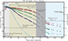 |
Fig. 1. Optical wavelength light curves of an example SN II together with the labelling of the different light curve phases. The distinct shaded regions are used to define where different physical processes dominate the luminosity of SNe II (see details in text). The generic naming scheme used in the literature to label these phases is given, together with observational parameters used to characterise those phases in brackets (from A14 and Gutiérrez et al. 2017b). It should be noted that phase boundaries are not necessarily well defined – they change between different SNe II, and are shown here as distinct abrupt changes for visualisation purposes. (While ‘SBO’ – shock breakout – is labelled on this plot and discussed in the text, it is not observed for this example SN II, nor for any other event in our sample). |
It is generally agreed that massive stars end their lives through ‘core-collapse’ (CC) – leading to a SN explosion. Massive stars go through successive stages of nuclear fusion (Hoyle 1954), burning heavier elements until an iron core forms. At this stage it is no longer energetically favourable to continue this burning sequence. The iron core grows until it reaches the Chandrasekhar mass and can no longer support itself against gravitational collapse. The core collapses until the inner core reaches nuclear densities. At such densities the strong nuclear force abruptly halts the collapse leading to a shock wave that propagates out through the still collapsing outer core. It is theoretically understood that this shock wave stalls, and a successful CC SN only ensues if the shock can be revived. The currently favoured scenario to produce a successful explosion is the ‘delayed neutrino driven mechanism’ (see e.g. Janka et al. 2017; Pejcha 2020; Burrows & Vartanyan 2021 and Fryer 2022 for reviews of CC SN theory – also see Soker 2019 for discussion of an alternative scenario). Once sufficient neutrino energy is captured, the shock wave is revitalised and can continue to propagate out through the rest of the star. From a physical perspective this can be considered the beginning of the SN (t0). However, at this stage no electromagnetic radiation can be seen by the observer3.
As the shock propagates outwards it accelerates and heats the stellar envelope. Once the shock arrives to the stellar surface, an intense flux of photons is able to leak out, producing the first electromagnetic radiation signal observed, known as the ‘shock break-out’ (SBO; e.g. Chevalier 1976; Falk & Arnett 1977; Ensman & Burrows 1992, see review by Waxman & Katz 2017). At SBO the SN undergoes a rapid increase in its luminosity. The duration of this transient feature is very short and depends on the size of the progenitor star. In the case of SNe II – with RSG progenitors – it is thought to last up to a few hours. While this is longer than for other SNe (with more compact progenitors), it is still an observationally difficult timescale to detect, that requires an especially designed survey with very high observational cadence (we do not observe this phase in any event in our sample), with only a small number of claimed detections (Soderberg et al. 2008; Schawinski et al. 2008; Gezari et al. 2015; Garnavich et al. 2016; Bersten et al. 2018; Tominaga et al. 2019; Vallely et al. 2021). The time of SBO is shown on the extreme left of the light curve phase diagram in Fig. 1. It is observable at all wavelengths but its brightness is much higher at bluer bands (however the SBO is expected to be smeared out in the presence of significant circumstellar material, CSM, see Moriya et al. 2011 and further discussion below). After this initial phase, rapid expansion leads to cooling of the ejecta.
The second phase in SN II light curves is often referred to as ‘shock cooling’ and is shown in Fig. 1 to last more than 10 days. During shock cooling the peak in the optical light curves is observed. These peak luminosities are a consequence of the peak of the SN spectral energy distribution (SED) progressively moving to longer wavelengths (lower temperatures) – thus SNe II peak earlier in bluer bands (Fig. 1, see also González-Gaitán et al. 2015). After light curve maximum (Mmax), SNe II show an initial decline in their brightness (s1). This decline continues until the third phase of the light curve is reached – the plateau. The time between initial explosion and the end of this shock-cooling phase has been referred to as Cd (the ‘cooling duration’; Gutiérrez et al. 2017b), and lasts several weeks. Until recently, it was thought that SNe II explode into a relatively clean environment, and thus their observed properties were not significantly affected by interaction between the ejecta and any surrounding material. However, there is now mounting evidence that many (and possibly the majority) of SNe II undergo interaction between the ejecta and CSM or an extended envelope (e.g. Khazov et al. 2016; Terreran et al. 2016; Yaron et al. 2017; Bruch et al. 2021) that is sufficiently strong to affect their early time light curves (González-Gaitán et al. 2015; Morozova et al. 2017; Förster et al. 2018). Hence, in Fig. 1 it is noted that the shock-cooling phase may also be powered by CSM interaction (in which case it is expected to last significantly longer).
At the end of the shock-cooling phase and the onset of the plateau, the outermost regions of the ejecta have reached temperatures of around 6000 K and the initially ionised hydrogen envelope starts to recombine (thus the plateau is also referred to as the ‘recombination phase’; see Faran et al. 2019 for an analytic discussion), and the decline rate (s2) starts to slow down considerably. During this phase hydrogen is recombined at different layers of the SN II ejecta. The recombination reduces the opacity – dominated by electron scattering – allowing the energy to diffuse outwards more easily. Recombination is the physical mechanism responsible for the escape of radiation. However, the energy released by the recombination process itself is only a small fraction of the radiated energy. The radiated energy is dominated by the energy stored in the SN ejecta initially deposited by the shock wave during its propagation through the stellar interior. Additionally, the late-plateau phase can be partially powered by the emission from the radioactive decay of 56Co. The exact moment when this contribution starts to affect SN II light curves depends on the degree of mixing of the radioactive material into the ejecta (see Bersten et al. 2011; Kozyreva et al. 2019).
At this stage in the description a note is required. The plateau phase is often referred to in the literature as ‘a phase of almost constant luminosity...’. However, a minority of SNe II show such behaviour (see detailed discussion in A14 and Sect. 5). Instead, SNe II show a large range in their plateau decline rates (s2) – some even increasing in optical luminosity (e.g. SN 2006bc, as will be shown in Fig. 13), and others declining by up to several optical magnitudes before the end of the plateau (see Fig. 18, later in the paper). Thus, it is more accurate to refer to the plateau phase (Pd in Fig. 1) of SN II evolution as ‘a phase of slowly changing luminosity relative to previous and subsequent phases, that lasts several months’. (Indeed, the example shown in Fig. 1 displays a clear plateau that declines relatively quickly). This plateau is more prominent in the redder optical bands (Fig. 1), and in some cases is observed as a slight increase in brightness (e.g. Fig. 13).
As a SN II evolves through its plateau the hydrogen recombines within increasingly inner layers of the envelope, and the photosphere moves inwards in mass coordinates following the recombination wave. At the end of the plateau (where one may also characterise the SN II through its magnitude Mend) the recombination wave has travelled to the inner edge of the hydrogen envelope. When this happens a sharp drop is observed in the light curve. This starts the fourth phase in Fig. 1 – the ‘transition’, where the powering mechanism transitions from being dominated by shock energy released by the recombination process to radioactivity on the tail. (The total phase from explosion to the end of the plateau is also referred to as the photospheric phase, defined as OPTd in A144.) This transition from a plateau to tail phase is observed in nearly all SNe II with sufficiently well observed light curves (see discussion in A14 and Valenti et al. 2015). Thus, there are very few (if any) true fast-declining SNe II that show light curves following the initial IIL description defined by Barbon et al. (1979). Even the classic prototypes, SN 1979C (de Vaucouleurs et al. 1981) and SN 1980K (Buta 1982; Barbon et al. 1982), show evidence for a transition phase (see Fig. 18 in A14).
During the last phase shown in Fig. 1, radioactive decay of 56Co (as the daughter product of 56Ni produced in the explosion) is the dominant power source5. Emission from radioactive decay is trapped by the ejecta and thus the s3 tail follows the decline rate expected by the decay rate of 56Co (at least in the majority of cases, although see A14 and Martinez et al. 2022a). During this phase the luminosity of a SN II (characterised by Mtail) is a direct indicator of the 56Ni mass ejected by the SN. In addition to changes in the light-curve shape, spectral properties also significantly transition as the continuum decreases in strength and the dominant features change (see Gutiérrez et al. 2017a for further details). During the radioactive tail a SN II gradually enters a ‘nebular phase’ where the inner core of the ejecta is revealed, the continuum becomes very weak, and spectra become dominated by emission lines.
At much later times, radioactivity from other elements starts to dominate the observed luminosity (e.g. 44Ti at around 1500 days post explosion, Suntzeff et al. 1992), and additionally dust formation (Matsuura et al. 2015) may produce a change in SN colour with NIR excesses observed (typically observed several hundred days post explosion). However, our data set does not extend to such late epochs and hence we end our light curve phase discussion here. In the next section the properties of our SN II photometric data sample are outlined.
3. The CSP SN II sample
3.1. The Carnegie Supernova Project: Aims and follow-up criteria
The data presented in this paper were acquired through the CSP over two distinct observational SN follow-up programmes. CSP-I (Hamuy et al. 2006) operated between 2004 and 2009 and obtained data for 74 SNe II. The overall aim of CSP-I was to obtain a foundational dataset of optical and NIR light curves of all types of SNe in a well-defined and understood photometric system6 (Hamuy et al. 2006). CSP-I SN follow-up was initiated on SNe discovered before or near to the epoch of maximum brightness, that occurred at low redshifts (i.e. z < 0.08), at declinations of less than 20° (in order to be observed from the Las Campanas Observatory, LCO), and that were estimated to reach an apparent optical magnitude of 18 or lower. Once follow-up was initiated, optical and NIR photometry together with visual-wavelength spectroscopy were obtained with relatively high cadence (see Sect. 3.4) until each SN was no longer sufficiently bright to continue observations, or it went behind the Sun.
CSP-II (Phillips et al. 2019) observed between 2011 and 2015 with a focus on obtaining optical and NIR photometry for SNe Ia in the smooth Hubble flow. Thus, it was not a major aim of CSP-II to observe SNe II. However, when nearby well-positioned (on the sky) SNe II were discovered, CSP-II obtained data for 20 such events. A new focus in CSP-II was to obtain NIR SN spectroscopic sequences for a statistically meaningful sample of SNe Ia (Hsiao et al. 2019). NIR spectral sequences were also obtained for a number of SNe II and were analysed and discussed by Davis et al. (2019): we display one such sequence in Sect. 5 (Fig. 15). CSP-II photometric follow-up of suspected SNe Ia in the Hubble flow often started before spectroscopic typing. Therefore, in a few cases relatively high-redshift SNe II were observed (see Fig. 2), but follow-up was stopped once their nature was confirmed leading to only a small amount of data per SN (e.g. for LSQ11gw and LSQ12fui). However, the majority of CSP-II SNe II are at lower redshift where high-quality optical and NIR light curves were obtained and in some cases NIR spectral sequences.
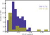 |
Fig. 2. Redshift distributions of the CSP-I and CSP-II SN II samples. The number of events in each subsample is given in brackets. |
Details of the combined CSP-I and CSP-II SN II samples, their discovery and classification, and additional information can be found in a Table on Zenodo7 (see the link in the data availability section). Discussion of the properties of the SN II sample is presented in Sect. 3.4. Now we summarise how CSP SN II optical and NIR photometry were obtained, reduced, and calibrated.
3.2. Data: Observations and processing
All photometric data presented here were obtained at LCO. The CSP instrumental set-up, SN and standard-star imaging acquisition, data reduction, and photometric calibration has been extensively outlined and analysed elsewhere (see below). We therefore do not repeat much of the detail in this paper. Here, we briefly describe all of the important concepts, but refer the reader to the relevant previous CSP data-release papers for specific details.
All CSP-I SN II optical imaging (uBgVri) was obtained with the 1 m LCO Swope telescope and the LCO Irénée du Pont (‘du Pont’) 2.5 m telescope. Most optical imaging was obtained using the direct CCD camera ‘SITe3’ mounted on the Swope, with a small number of images obtained using the facility ‘Tek5’ CCD camera mounted on the du Pont. The majority of host-galaxy template images (obtained once each SN had faded beyond detection) were obtained with the du Pont. NIR SN images (YJH) were mainly obtained with ‘RetroCam’, a NIR imager built specifically for the CSP-I and mounted on the Swope telescope. A small number of NIR images were obtained with the Wide Field IR Camera (WIRC) on the du Pont telescope. All host-galaxy template imaging in the NIR was obtained using WIRC. Hamuy et al. (2006) outlined the CSP-I instrumental setup in detail, while further presentation and discussion of system response functions can be found in Krisciunas et al. (2017) and Stritzinger et al. (2018). Following Stritzinger et al. (2018), we note that the V-band filter was changed for the Swope+SITe3 system during the course of CSP observations (on January 25th 2006), however the same colour term was shown to be applicable to both filters. Meanwhile, two different J-band filters were used on the Swope+RetroCam system: JRC1 before January 15th 2009, and JRC2 afterward. The derived colour terms for these filters were found to be sufficiently distinct to warrant publication of SN photometry on two different systems.
The systems used to obtain photometry for CSP-II were very similar to CSP-I, but with a few important differences that are now outlined (see Phillips et al. 2019 for a full description). During the first two observing campaigns (yearly observing seasons) of CSP-II, the same Swope+SITe3 system was used to obtain optical photometry as during CSP-I. Then, for the third and fourth campaigns the detector was replaced by a new e2V deep-depletion CCD (see Phillips et al. 2019 for a comparison of the system throughputs in combination with the employed filters). CSP-II also used the du Pont+Tek5 system to obtain a small number of follow-up images, together with the optical host-galaxy reference images. At the start of CSP-II, the NIR imager RetroCam was moved from the Swope to the du Pont, and thus CSP-II, NIR imaging was obtained using du Pont+RetroCam. In addition, during CSP-II NIR host-galaxy template images were obtained mostly using FourStar (Persson et al. 2013) on the Magellan Baade telescope, with a small number obtained using du Pont+RetroCam.
The full CSP data workflow is detailed by Contreras et al. (2010) and Stritzinger et al. (2011) (the first and second SN Ia data releases, respectively). All images (science, standard star, host-galaxy templates) were processed in the standard manner, including bias subtractions, flat-field corrections, linearity correction, and correction for a shutter time delay to the exposure time. Host-galaxy template images – obtained when the SN had faded from detection and in excellent observing conditions – were used to subtract the contribution of galaxy light from the SN. Details of this process and a discussion of possible systematic errors involved can be found in Contreras et al. (2010) and Folatelli et al. (2010). Photometry was then computed for local sequence stars within the field of view of each SN image (in the optical or NIR), and these sequences were calibrated with respect to standard-star fields observed on at least three photometric nights. This strategy and procedure is outlined by Krisciunas et al. (2017). Photometry of local sequence stars is on the standard systems of Smith et al. (2002) for ugri, Landolt (1992) for BV, and Persson et al. (1998) for JH, while Y is calibrated to the system defined in Krisciunas et al. (2017).
All CSP definitive photometry has been and will be released in the natural system of the telescope and instrumental setup of the observations. This is done to avoid major issues in using colour terms derived from stars to transform SN photometry into a standard photometric system. To achieve the former, local sequence photometry is transformed to the natural system using the formulation presented by Krisciunas et al. (2017). Definitive natural-system point spread function photometry for SNe II is then derived with respect to these natural local sequences. Final photometric uncertainties are estimated by combining the instrumental magnitude error of each individual SN photometric point with that on the nightly zero point. Our published photometric errors do not therefore include systematic uncertainties such as those arising from host galaxy flux subtraction. The reader is again referred to Contreras et al. (2010) and Krisciunas et al. (2017) for a full description of the origin of photometric uncertainties and analyses of the accuracy and precision of CSP photometry.
Photometry for the full, final optical and NIR light curves of 94 SN II from the CSP, together with photometry of local sequences is discussed in the Sect. 4. We first outline how we estimate explosion epochs for our sample in the next subsection. Then, we present general properties of our SNe II that elucidate the nature of our sample, and additionally summarise previous analyses achieved with these SN II data sets, before presenting our SN II photometry in Sect. 4.
3.3. SN explosion epochs
A key parameter to analyse any sample of SNe is the assumed date of explosion. This is important for (e.g.) SN modelling and extraction of physical parameters of their explosions, and for the use of SNe II to measure distances. To estimate explosion epochs for our SNe II we follow the same methodology as Gutiérrez et al. (2017a) and apply this to both the CSP-I and CSP-II samples. Gutiérrez et al. (2017a) already estimated explosion epochs for most of the CSP-I sample. We re-check those values in this work and the majority of epochs published here are consistent with that previous work (see Table on Zenodo through the link given on the data availability section). If a constraining nondetection exists8 less than 20 days before discovery then this is used to estimate the time of explosion. The explosion epoch from this ‘N’, nondetection method is then taken to be the mid point between the nondetection and the first detection, with the error being that time range divided by two.
It is important to note that the uncertainties presented on our ‘N’ explosion epochs are not Gaussian. Without any additional knowledge of (for example) the photometric rise to maximum or the exact magnitudes of the nondetection limit and the discovery detection, such errors should be understood to mean that there is an equal probability that the SN exploded at any time t between the nondetection and the first detection (i.e. the explosion time ± the error). However, for each individual SN II, one does have additional information, the most relevant of which (for the current sample) is the difference in magnitude between the nondetection and the first detection. If the nondetection limit is close in magnitude to the first detection, then it is not particularly constraining, leaving the possibility that the SN exploded close in time or even before the nondetection. The deeper the nondetection the more constraining it becomes that the event exploded after that limit. While we do not use such information to more precisely constrain explosion epochs in this work, details of this photometry are listed in the Table available on Zenodo (see the link in the data availability section) so that the reader can assess each specific SN II constraint on the merits of its data.
In the case where no constraining nondetection exists (i.e. any such data are more than 20 days before the first detection), then spectral matching (‘S’) is used to constrain explosion epochs. Spectral matching refers to the technique of comparing a spectrum or a spectral sequence of a given SN to those from a library of template spectra of observed SNe with well-constrained explosion epochs. Several tools have been developed to perform this task, and here we use the Supernova Identification (SNID) code (Blondin et al. 2007). For a full overview of our use of SNID please refer to Sect. 4 of Gutiérrez et al. (2017a).
Similarly to the nondetection method, there are also caveats to the use of spectral matching to obtain accurate explosion epochs. Libraries of spectral templates are often lacking in spectra of peculiar objects meaning that constraints for any such objects may be less reliable. Gutiérrez et al. (2017a) compared the differences between explosion epochs estimated through the nondetection (N) and spectral matching (S) techniques for objects with good constraints from both. Good agreement was found, with a mean absolute error between techniques of less than four days and a mean offset of 0.5 days (the latter indicates that there is no systematic offset between the techniques in one particular direction). For a subset of the SNe II presented in this work, the explosion epochs from the above techniques were compared to those obtained from hydrodynamical modelling of their bolometric light curves and spectral velocities in Martinez et al. (2022b). The mean offset between our ‘observational’ explosion epochs and those estimated through modelling is close to zero, indicating that there is no systematic offset between the different methodologies9. Following the above, while for any specific SN there may be some peculiarities in its data (photometry, spectra) meaning that its explosion epoch is somewhat in error, no systematic issues have been found in applying our employed explosion epoch estimation methodology.
3.4. Properties of the CSP SN II photometry sample
Information on the SNe II contained within this CSP data release, discovery and classification references, together with the number of data per SN are given in a Table on Zenodo (see the link in the data availability section). As outlined above, a SN II was considered for follow-up by both CSP campaigns if it was discovered before or close to maximum light and if it was bright enough for high-quality data to be acquired. This defines the sample as magnitude limited, while SN discoveries were provided by a large number of different surveys. SNe II observed by CSP-I were mostly discovered by galaxy-targeted surveys (88%), as during the 2004–2009 discovery epoch most nearby SNe were still discovered by such programmes (see appendix of A14). This led to a sample with very few SNe II in low-luminosity galaxies (see Fig. 22 of A14). SN type and property distributions can change significantly when found in different luminosity galaxies (see, e.g. Arcavi et al. 2010). Indeed, SNe II found within lower luminosity hosts (i.e. lower than the distribution of the A14/CSP-I sample) show intriguing differences compared with those events found in brighter galaxies (see, e.g. Taddia et al. 2016; Gutiérrez et al. 2018; Anderson et al. 2018; Scott et al. 2019). Such differences are possibly linked to the effects on stellar evolution of SNe II arising from lower metallicity progenitors (implied from the lower luminosity of their hosts). CSP-II meanwhile was executed when a number of large-field-of-view surveys had come on line, that scanned the sky in an untargeted fashion. The CSP-II sample contains only 40% of objects discovered by targeted surveys. SN 2015bs – part of the CSP-II sample – is one clear example of a SN II that would have been missed by galaxy-targeted surveys given its extreme low-luminosity host. This object had very weak metal lines in its optical-wavelength spectra – indicative of a low-metallicity progenitor, together with very strong oxygen lines at nebular times – indicative of a relatively massive progenitor (Anderson et al. 2018). It is important to keep the above sample selection issues in mind when comparing the current sample to other SN II data sets in the literature.
In Fig. 2 we plot the redshift distribution of the sample, separating events into CSP-I and CSP-II. The full sample has a median redshift of 0.015 with a maximum of 0.07 (LSQ12fxu, that was initially observed as part of the ‘SN Ia cosmology sample’ for CSP-II), and a minimum of 0.00075 (SN 2008bk). As can be seen in Fig. 2, apart from a few higher redshift events (initially suspected of being SNe Ia), the CSP-II sample generally concentrates at lower redshift than CSP-I. This was by design, as CSP-II only initiated significant SN II follow-up for the closest events – where NIR spectral sequences could be obtained.
Here we present a total of 9817 optical (uBgVri) photometric measurements for 94 SNe II (7716 for CSP-I and 2101 for CSP-II). Meanwhile, in the NIR (YJH), 1872 data points are presented (1705 for CSP-I and 167 for CSP-II). For the full (CSP-I + CSP-II) sample, SNe II have a median of 93 optical photometric points and a median number of NIR points of 18. All 94 SNe II have at least some optical photometry, while 77 (62 CSP-I and 15 CSP-II) have NIR light curves. Figure 3 displays the distribution of the number of distinct photometric data points. The largest optical data set is of 506 photometric measurements (SN 2013hj), while the minimum is of 7 (LSQ12fui). In the NIR, SN 2008ag has the most data points (61), while there are a number of events without any data at NIR wavelengths. The sample has a median V-band cadence of 4.7 days – over a median optical-photometry coverage of 79.9 days. In the NIR the median J-band cadence is 7.2 days over a NIR coverage of 58.9 days.
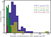 |
Fig. 3. Number of optical (uBgVri) and NIR (YJH) photometric data points per SN for the CSP-I and CSP-II SN II samples. The number of events in each subsample is given in brackets. |
The epochs of the earliest and latest optical and NIR photometry per SN are displayed in Figs. 4 and 5 respectively. The earliest photometry obtained at optical and NIR wavelengths is within two days of the estimated explosion epoch (SN 2008gr). The inset in Fig. 4 shows a zoom of the first 13 days post explosion. For CSP-I only a small number of SNe II have their first photometric point within less than five days from explosion. However, for CSP-II almost half the sample have such early time data. This is a consequence of the evolution of transient surveys – during CSP-I it was still relatively rare to discover SNe within a few days of explosion. Post CSP-I (and during CSP-II) survey capabilities significantly improved and more SNe were (and are) found at such early epochs. The latest optical photometry was obtained for SN 2013hj at 500 days post explosion, while in the NIR data were obtained at 419 days post explosion for SN 2008bk. The majority of the CSP-I sample have accompanying visual-wavelength spectral sequences (presented and analysed by Gutiérrez et al. 2017a,b), while the CSP-II SNe II have at most one or two optical spectra, but several have well-sampled NIR spectroscopy (Davis et al. 2019). The number of spectra and the range of their epochs for each SN II is listed in a Table on Zenodo (see the link in the data availability section), while the epochs of the spectra are depicted on each light curve that are also presented on Zenodo.
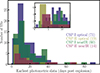 |
Fig. 4. Distribution of the epochs of the earliest optical and NIR photometry obtained (with respect to explosion epoch) for each SN in our sample. The number of events in each subsample is given in brackets. The inset shows a zoom into the first 13 days post explosion. |
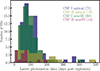 |
Fig. 5. Distribution of the epochs of the latest optical and NIR photometry obtained (with respect to explosion epoch) for each SN in our sample. The number of events in each subsample is given in brackets. |
3.5. Previous analyses achieved with the CSP SN II samples
Before presenting and discussing the multiwavelength light curves released in this work, here we briefly summarise the previously presented analyses that have used these data (and in some cases also published preceding releases of photometry10). We do this to (a) aid the interested reader in surveying the CSP SN II literature, and (b) give context to the subsequent qualitative discussion in the latter sections of this paper. Papers are discussed in chronological order.
As described above, Hamuy et al. (2006) presented the first instalment of the CSP – describing the survey and reduction methodology while also presenting example photometry from the first few years of the project. Specifically, light curves and spectra were presented for the type II SN 2004fx (see Fig. 11 in the current paper). Takáts et al. (2014) analysed the ‘intermediate luminosity’ SN 2009N, constraining its progenitor properties through hydrodynamical modelling and additionally using the SN observations to constrain the distance to its host galaxy, NGC 4487.
The current data release is a natural succession to the V-band data release in A14. A14 characterised the V-band light curves of SNe II, investigating the observed diversity within a large sample (more than 100 events when including the data published by Galbany et al. 2016). That work defined different light-curve properties including, absolute magnitudes, decline rates, and durations of different phases – concluding that SNe II form a continuum in their light-curve properties with no evidence for distinct photometric groups. Gutiérrez et al. (2014) tied these photometric properties to the morphology of the dominant Hα spectral line, finding that faster declining SNe II displayed much weaker Hα absorption than slowly declining explosions. Dessart et al. (2014) compared observations to model spectra of distinct progenitor metallicity suggesting that most of the current sample arose from stars with solar metallicity, with a lack of low-metallicity events, which is unsurprising given that the CSP-I objects are mainly SNe II discovered by means of targeted surveys. Anderson et al. (2014b) again concentrated on the trademark SN II spectral feature – Hα. There, we demonstrated that the peak emission of this feature is generally blueshifted with respect to zero rest velocity, a property that is reproduced by the models of Dessart et al. (2013) and can be understood as being tied to the steep density profiles of SN II ejecta.
CSP-I photometry was used by de Jaeger et al. (2015) to show that luminosity distances can be calculated when only using SN II photometry – an important finding in the current and future eras of wide-field surveys where many more transients will be detected than one can follow-up spectroscopically. Following the work of Dessart et al. (2014), in Anderson et al. (2016) the CSP-I SNe II spectral and photometric properties were compared to oxygen abundances of host H II regions. SN II metal-line strength was shown to correlate with environment elemental abundance, strengthening the case for the use of SN II to measure galaxy metallicities. The Photometric Color Method (PCM) introduced by de Jaeger et al. (2015) was later used by de Jaeger et al. (2017b), where CSP SNe II were combined with higher redshift samples to produce a Hubble diagram and measure cosmological parameters.
As previously noted, visual-wavelength spectroscopy of the CSP-I SN II sample was published by Gutiérrez et al. (2017a). Subsequently, Gutiérrez et al. (2017b) compared a large range of spectral-line measurements to photometric parameters. This analysis showed that SNe II with higher expansion velocities are more luminous, and had more rapidly declining light curves, shorter plateau durations, and higher 56Ni masses.
CSP-II photometry of SN 2015bs was published by Anderson et al. (2018), where photospheric- and nebular-phase spectra were used to show that its progenitor had the lowest metallicity and highest mass of any SN II studied to-date. de Jaeger et al. (2018) argued that dispersion seen in SN II observed colours is dominated by intrinsic colour differences of the explosions and not by the effects of host-galaxy extinction. Pessi et al. (2019) compared the optical light curves of SNe II (from the CSP-I) to literature SNe IIb, showing that there is no continuum between the properties of the fastest declining hydrogen-rich SNe II and SNe IIb – suggesting distinct progenitor channels for the two groups.
The CSP-II obtained NIR spectra for a significant fraction of the sample SNe II. These were analysed – together with photometry – by Davis et al. (2019). Distinct spectroscopic families were found, somewhat in contradiction to the clear continuum of events observed in photometry (A14). CSP data of SN 2008bm, SN 2009aj, and SN 2009au were published by Rodríguez et al. (2020), who found that these three events were initially powered by significant ejecta-CSM interactions, boosting their luminosity while slowing down their expansion velocities. Finally, data of SN 2006Y (see our Fig. 22) and SN 2006ai (Fig. 17) were presented by Hiramatsu et al. (2021), where it was concluded that RSGs with enhanced mass loss are required to produce their light curves (specifically their ‘short plateaus’; see also Martinez et al. 2022c).
Together with this data release, we have also published an additional three studies by Martinez et al. (2022a,b,c) (respectively M22a, M22b and M22c henceforth) using the CSP-I SN II sample. First, in M22a we present bolometric light curves for all events and outline a methodology for accurately estimating the bolometric flux for any given SN II. This paper shows the importance of using NIR photometry for such estimates and gives corrections to use when such data are unavailable. Together with the spectral velocities published by Gutiérrez et al. (2017a), bolometric light curves are used to determine progenitor and explosion parameters of the SN II sample in M22b through comparison to hydrodynamical models (following the procedure of Martinez et al. 2020). Specifically, we derive ZAMS masses for the sample, finding a bias towards low progenitor mass. Finally, in M22c we correlate physical parameters from the best-fit models to observed transient parameters to further understand the underlying physics driving SN II diversity. In Sect. 5, we quote the results of these studies when comparing specific events in our sample to the general SN II phenomenon.
4. Ninety-four SN II multiband light curves
In this section, we present an example SN II: showing SN and local-sequence photometry, a finder chart, and the uBgVriYJH optical to NIR wavelength light curves. Complete electronic, machine readable tables of SN and local-sequence photometry can be downloaded from the CDS11, and finder charts and light curves for our full sample of SNe II can be found on Zenodo through the links in the data availability section. After showing an example case, we characterise the CSP SN II sample in terms of its observed parameters in the V band (following A14), and define a small SN II comparison sample to put our sample within the context of the literature.
Throughout the rest of the paper, light curves are depicted with respect to their explosion epochs (while tabulated photometry is with respect to Julian date). Explosion epochs (and their uncertainties) together with information used to constrain them are listed for each SN II in a Table on Zenodo (see the link in the data availability section). Light curves in figures are displayed in both apparent and absolute magnitudes. Apparent and absolute magnitudes are corrected for Milky Way extinction taken from Schlafly & Finkbeiner (2011), assuming the extinction law from Cardelli et al. (1989) with RV = 3.1 (but published photometry is not corrected). Absolute magnitudes are calculated using distance moduli taken from A14 and Davis et al. (2019) (or derived using the same methodology). Light curves are not corrected for host galaxy extinction as we believe that in most cases these are small (< 0.1 mag) and any corrections employed are generally unreliable (see de Jaeger et al. 2018). Uncertainties on individual photometric measurements are shown in the figures, but are often too small to be visible on the plots.
4.1. An example of CSP SN II photometry: SN 2007oc
Figure 6 displays the finder chart for SN 2007oc, with optical local sequence stars labelled. Local-sequence optical and NIR photometry are listed in Tables A.1 and A.2, respectively. This local-sequence photometry is published in the standard system of Smith et al. (2002) for ugri, the standard system of Landolt (1992) for BV, the standard system of Persson et al. (1998) for JH and the natural system of the Swope+RetroCam setup for Y (defined as the ‘standard’ system for Y-band photometry by Krisciunas et al. 2017). The apparent and absolute magnitude light curves of SN 2007oc are shown in Fig. 7. SN photometry is published in the natural CSP systems, and optical photometry is given in Table A.3, while NIR photometry is given in Table A.4.
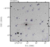 |
Fig. 6. Finder chart of SN 2007oc with the SN position marked with a red cross, while optical local sequence stars are marked with blue circles. (Such finder charts for all SNe II in our sample can be found on Zenodo through the link in the data availability section). |
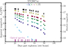 |
Fig. 7. uBgVri and YJH apparent and absolute magnitude light curves of SN 2007oc plotted relative to the explosion epoch. Epochs when visual-wavelength spectra were obtained are indicated on the abscissa. (Such light curves for all SNe II in our sample can be found on Zenodo through the link in the data availability section.) |
SN 2007oc has extremely well-sampled optical and NIR photometry between around 25–80 days post explosion, but is missing data at early and late times. This SN II has a relatively fast declining light curve with an s2 of 1.8 ± 0.01 mag /100 d and a relatively short photospheric phase with an OPTd of 71 ± 5 days (see Figs. 8 and 9 for reference, and see below for a description of how these parameters are defined and measured).
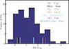 |
Fig. 8. V-band s2 distribution for the CSP and comparison samples. The comparison sample values are shown as ticks on the abscissa. |
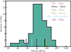 |
Fig. 9. OPTd plateau duration distribution measured in the V band for the CSP and comparison samples. The comparison-sample values are shown as ticks on the abscissa. (ASASSN-15nx is not shown here as it was not possible to define the end of any plateau phase – there is no discernible break to the post maximum decline rate out to late times). |
4.2. Sample characteristics and comparison-sample definition
In A14 we presented a characterisation of the V-band light curves of SNe II, including many of the events for which we publish photometry here. A14 attempted to capture the main parameters of SN II light curves through defining a number of absolute magnitudes at different times, decline rates at different epochs, and durations of different phases. In the current work we also use the V band for easy comparison, and concentrate on two parameters that have historically defined the discussion of SN II light-curve morphology: the plateau decline rate, parameterised here through s2 (the decline rate of the second, slower decline in the light curve post maximum light), and the duration of the plateau, parameterised here through OPTd (the time from explosion to the end of the plateau)12, both measured in the V band. Following A14, s2 is measured by fitting a piecewise linear model with four parameters: the decline rates s1 and s2, the epoch of the inflection between these points ttran, and the magnitude offset. The start of s1 and the end of s2 are visually defined and the values of the decline rates and their inflection point are determined through weighted least squares minimisation. The Bayesian Information Criterion (BIC, Schwartz 1978) is used to evaluate if the data are better fit by one slope (that is then assigned to be s2) or two (s1 and s2). The SN II parameters s2 and OPTd are listed for all SNe in a Table on Zenodo (see the link in the data availability section).
Throughout the subsequent discussion we select a group of SNe II from the literature for comparison. These events are selected by being either well-known literature SNe II or because they have specific characteristics that enable us to put the current sample within the context of the observed diversity of SNe II. While the reader should note that this selection is subjective, the comparison sample is not used to derive strong conclusions on the nature of SNe II and thus its exact nature is somewhat unimportant. In order of discovery, the comparison sample is, SN 1979C, SN 1999em, SN 1999gi, SN 2005cs, SN 2013ej, SN 2014G, and ASASSN-15nx. SN 1979C (de Vaucouleurs et al. 1981) is often cited as the historical example of a SN IIL fast decliner, and thus we include it here. This event was extremely bright; it was more luminous than any SN II in the current sample. SN 1999em (e.g. Hamuy et al. 2001; Leonard et al. 2002b) and SN 1999gi (e.g. Leonard et al. 2002a) are prototypical slow decliners (IIP) showing all the common characteristics that are discussed as belonging to the SN II phenomenon. Specifically SN 1999em is often used as the standard event for model comparison (e.g. Utrobin 2007; Bersten et al. 2011; Dessart et al. 2013). SN 2005cs is one of the best-observed ‘low-luminosity’ SNe II (Pastorello et al. 2006; see Spiro et al. 2014 for a sample analysis). Such events generally show low ejecta velocities in combination to their dimness. SN 2013ej has been called both a IIP and IIL in the literature (e.g. Valenti et al. 2014; Bose et al. 2015; Huang et al. 2015; Dhungana et al. 2016; Mauerhan et al. 2017), as it shows a relatively fast declining light curve but also a clear plateau (as do nearly all hydrogen-rich SNe II). We therefore include this in our comparison sample as an ‘intermediate’ SN II. SN 2014G (Terreran et al. 2016) is included as another example of a fast decliner (but which again shows a clear plateau). Finally, ASASSN-15nx is possibly the only hydrogen-rich SN II in the literature with a true ‘linear’ decline post maximum light (Bose et al. 2018)13. We therefore include this event for comparison as the most extreme hydrogen-rich SN II: a bright SN II, with a fast declining light curve and no apparent plateau phase.
Figure 8 shows the V-band s2 distribution of the CSP sample together with our comparison sample. The majority of SNe II decline between zero and two magnitudes per 100 days before the end of the plateau. A few events have negative s2 values – they increase in optical brightness during this phase. A small number of events decline faster than 2.5 mag /100 d. Further discussion of the fast decliners is presented below.
Figure 9 shows the OPTd distribution. A strong peak is observed around 90 days and the vast majority of events arrive to the end of their plateau between 75 and 100 days post explosion. A tail is seen at low OPTd (see discussion in Sect. 5), and a few SNe II do not drop from the plateau until almost 120 days after explosion.
Figure 10 displays CSP SN II uViH absolute magnitude light curves for a subsample of our SNe that are well-observed. These bands are chosen to show the different light-curve evolution as one moves from the bluest (u) through to the reddest (H) wavebands. It is clear that SN II light-curve evolution is much faster at bluer wavelengths – the u-band luminosity falls off quickly post maximum and plateau phases are almost nonexistent. In V the figure shows the typical light-curve morphology of SNe II: post maxima flat or slowly declining light curves until arriving to the end of the plateau. In i one starts to observe a larger fraction of SNe II that increase in luminosity during the plateau phase. In the NIR H band, SN II light curves show much longer rise times to maximum, and light curves display a more round and gradual evolution than observed at visual wavelengths.
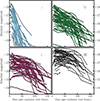 |
Fig. 10. uViH absolute magnitude light curves of CSP SNe II. Individual photometric points have been joined by lines to provide a visualisation of the different light curve morphologies observed at different wavelengths. |
5. Discussion
This discussion section is devoted to summarising the properties of a number of specific SNe II in the CSP samples, helping to put these events – and indeed literature SNe II – in some context. In the following, we present absolute magnitude light curves and spectral sequences for different explosions that capture the main diversity of SNe that form the SN II class. In addition, we highlight a number of nonstandard SNe II and discuss their unusual properties. Visual-wavelength spectral sequences of the CSP-I sample were presented by Gutiérrez et al. (2017a), while for CSP-II SNe II we have at most a few such spectra. On the contrary, there are no NIR spectra of the CSP-I SN II sample, but many CSP-II SNe II have well-observed NIR spectral sequences (see Davis et al. 2019). We discuss these example events in terms of their V-band light-curve morphologies and spectral ejecta velocities, and any other peculiarities and/or interesting features that each SN displays. The comparison sample introduced in the previous section is again highlighted, where it aids the reader in comprehending each example SN. As we have not made any host-galaxy extinction corrections to our CSP SN II sample, we also ignore such effects for the literature comparison SNe for internal consistency.
Where relevant the explosion and progenitor estimates for our SNe II from M22b are also stated below. In this regard, it is important to note that the modelling in M22b assumed standard single-star stellar evolution to produce pre-SN progenitors that were then exploded. Changes in such assumptions can lead to distinct estimates on progenitor and explosion properties compared to observations (see e.g. Dessart & Hillier 2019). In addition, the modelling in M22b did not include the effects of interaction between the SN ejecta and any surrounding CSM (see Morozova et al. 2018 who included such material in hydrodynamical modelling of SNe II, and Hillier & Dessart 2019 for an analysis of how differences in progenitor, explosion, and CSM properties may produce observed diversity in SN II light curves and spectra). M22b only modelled SN II light curves after 30 days post explosion, where it is assumed that any effects from earlier ejecta–CSM interaction are unimportant. Given that our sample also generally lacks data within the first few days post explosion, we also ignore discussion of CSM interaction below. However, the reader should be aware that such interaction may still be affecting the very-early time data (when available) and its interpretation, given the mounting evidence for such interaction in the majority of ‘normal’ SNe II (e.g. Förster et al. 2018; Bruch et al. 2021 and references therein). It is also possible that CSM interaction may be the source of some of the peculiar objects discussed at the end of this section.
Throughout this discussion we compare specific SNe II to the general population of light-curve and spectral properties using median values from Gutiérrez et al. (2017b). Specifically, we compare to the absolute magnitude at maximum light in the V band (Mmax, with a median value −16.7 mag), the plateau decline rate (s2, 1.1 mag/100 d), the duration of the plateau phase (OPTd, 87 days), the ejecta velocity from the absorption component of Hα at 50 days post explosion (Hα50, 7270 km/s), and the ejecta velocity from the Fe 5169Å line (Fe50, 3940 km/s). All individual SN II values are taken from Gutiérrez et al. (2017a), or are measured following the same methodology (however here we present s2 and OPTd values in the rest frame of each SN – in Gutiérrez et al. 2017a values were presented in the observer frame). We also use the physical parameter distributions from M22b to further elucidate the nature of each specific object.
5.1. Slowly declining SNe II
We define ‘slowly declining SNe II’ as those events showing a clear, relatively flat plateau that would generally be considered ‘normal’ SNe II by the community. Prototypical slowly declining events can be found in the literature as the well-known SNe 1999em and 1999gi, as already described in the previous section. In the following, we highlight CSP SNe II showing similarly classical SN II light-curve morphologies. However, we also note the diversity displayed even within this smaller subsample.
SN 2004fx: Optical and NIR photometry and the visual-wavelength spectral sequence of SN 2004fx are displayed in Fig. 11. This SN II exhibits a standard slowly declining light-curve morphology, with a very well defined plateau, transition and tail. The epoch of peak luminosity appears to have been missed (a common property of CSP-I SNe II) and any definition of an initially steeper post-maximum decline (s1) is unclear. The decline rate is quite slow, with an s2 of 0.25 ± 0.02 mag/100 d: much slower than the 1.1 mag/100 d median. SN 2004fx appears slightly subluminous for a slowly declining event, falling between SN 1999em and the low-luminosity SN 2005cs (Fig. 11). The light curve shows a slow transition from the plateau to the tail. The OPTd is noticeably shorter than in other slow decliners, with a value of 68 ± 6 days (compared to the 87 day median for the full sample). The spectral sequence displays typical features of SNe II – with strong formation of the Hα P-Cygni profile in the first spectrum at 23 days post explosion (+23 d). The modelling presented by M22b suggests a relatively low explosion energy (0.4 ± 0.01 foe14 compared to the 0.6 foe median), a low 56Ni mass (0.012 ± 0.001 M⊙, 0.036 median), and a low-mass progenitor (ZAMS mass of 10.0 ± 0.15 M⊙, 10.4 M⊙ median)15.
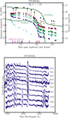 |
Fig. 11. Absolute and apparent magnitude uBgVri and YJH light curves (top) and visual-wavelength spectra (bottom) of SN 2004fx. The V-band absolute magnitude light curves of SN 1999em and SN 2005cs are also displayed for comparison. |
SN 2005J: Absolute magnitude light curves and the visual-wavelength spectral sequence of SN 2005J are displayed in Fig. 12. This SN II is more luminous than most other events, with an Mmax of −17.3 ± 0.1 mag. While the tail is not observed, this event still displays a typical light-curve morphology and has a decline rate of 1.1 ± 0.02 mag/100 d. Even though both SN 2005J and SN 2004fx would be considered ‘typical’ SNe II in terms of light curve morphology, visually the shapes of their luminosity evolution clearly differ – SN 2004fx displays a much more ‘rounded’ transition phase. In addition to being slightly more luminous, SN 2005J also displays larger spectral velocities than the general population, with an Hα50 of 8430 ± 760 km/s (median 7270 km/s) and an Fe50 of 4220 ± 440 km/s (median 3940 km/s). These properties suggest a more energetic explosion for SN 2005J, with the modelling of M22b giving an explosion energy of 0.8 ± 0.08 foe (and additionally a ZAMS mass of 15.4 ± 1.1 M⊙). Another interesting feature of SN 2005J is that it appears to show a long initial post-maximum decline before arriving to s2 (although while this is clearly visible in the B band in Fig. 12, it is not statistically observed in V).
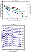 |
Fig. 12. Absolute and apparent magnitude uBgVri and YJH light curves (top) and visual-wavelength spectra (bottom) of SN 2005J. The V-band absolute magnitude light curve of SN 1999em is also displayed for comparison. |
SN 2006bc: Absolute magnitude light curves and the visual-wavelength spectral sequence of SN 2006bc are displayed in Fig. 13. While this SN II is not particularly well observed (the end of OPTd was not caught), one can immediately identify two defining features in its transient behaviour. After an initial slight decline in the optical photometry post peak, all wavebands redder than g show a clearly increasing luminosity during its OPTd. The s2 of SN 2006bc is −0.58 ± 0.04 mag/100 d, the most negative such value in our sample (Fig. 8). The SN is relatively faint, with an Mmax of −15.2 ± 0.3 mag (A14), and the spectra displayed in Fig. 13 show extremely narrow P-Cygni profiles (the last spectrum is at +30 d and thus we do no have values at the comparison epoch of 50 days post explosion). These SN properties probably imply a low explosion energy event; however, the data were deemed insufficient for reliable modelling and thus no physical parameters were extracted for SN 2006bc by M22b.
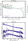 |
Fig. 13. Absolute and apparent magnitude uBgVri and YJH light curves (top) and visual-wavelength spectra (bottom) of SN 2006bc. The V-band absolute magnitude light curve of SN 2005cs is also displayed for comparison. |
SN 2008ag: Absolute magnitude light curves and the visual-wavelength spectral sequence of SN 2008ag are displayed in Fig. 14. Visually assessing this SN II one may conclude that this is a ‘prototypical’ slowly declining explosion. Indeed, while the first several tens of days of the transient evolution were missed, for the rest of its evolution it clearly shows features consistent with the literature definition of a normal SN II: an OPTd which lasts for several months (OPTd of 104 ± 9 days) where the luminosity stays relatively constant (s2 of 0.12 ± 0.03 mag/100 d). However, the SNe II highlighted in this subsection also clearly show that a large range of such events would be considered normal but display obvious differences in their light curves and spectra, suggesting differences in their progenitor and/or explosion properties. OPTd is relatively long for SN 2008ag compared with the general population (median 87 days), while its light curve is much flatter than in most SNe II (0.12 ± 0.03 mag/100 d compared to a median of 1.1 mag/100 d). In addition SN 2008ag is slightly brighter (Mmax of −17.0 ± 0.2 mag, compared to the −16.7 mag median). The spectral sequence displayed in Fig. 14 is typical of SN II line-formation evolution and its velocities are close to the median values. Modelling from M22b gives a high ZAMS mass of 20.9 ± 0.9 M⊙ (the highest extracted mass in the CSP-I sample) and an explosion energy of 0.9 ± 0.03 foe. These values are a consequence of the long and bright OPTd together with ‘normal’ velocities of SN 2008ag.
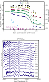 |
Fig. 14. Absolute and apparent magnitude uBgVri and YJH light curves (top) and visual-wavelength spectra (bottom) of SN 2008ag. The V-band absolute magnitude light curve of SN 1999em is also displayed for comparison. |
ASASSN-15bb: Finally, we show a SN II from the CSP-II (ASASSN-15bb) in Fig. 15. This is specifically shown to advertise an example of the NIR spectral sequences available for the CSP-II SN II sample (as presented and analysed in Davis et al. 2019). As with SN 2008ag, ASASSN-15bb shows a classical SN II morphology – both visually and quantitatively. As is common for the CSP-II sample, ASASSN-15bb was observed relatively early post explosion. After an unclear peak epoch this SN II had a relatively flat light curve during its OPTd, with an s2 of 0.48 ± 0.06 mag/100 d. Its photospheric phase had a typical length for a SN II of 82 ± 4 days, while it was relatively bright – being brighter than −17 mag (V) through the duration of OPTd. The NIR spectral sequence displayed in Fig. 15 is dominated by the Paschen series – as is normal for SNe II observed at such wavelengths and epochs.
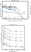 |
Fig. 15. Absolute and apparent magnitude uBgVri and YJH light curves (top) and NIR wavelength spectroscopy (bottom) of ASASSN-15bb. The V-band absolute magnitude light curve of SN 1999gi is also displayed for comparison. |
5.2. A new sample of fast-declining SNe II
SNe II show a continuum in the vast majority of their observational properties – there is no clear separation between slowly declining and fast-declining events (e.g. A14, Gutiérrez et al. 2017b). Thus, one may question the validity of discussing different subsets of the general SN II population. However, while a clear continuum exists in SN II light curve properties, the decline rate (s2) of a SN II correlates with many other photometric and spectral properties (see details in Gutiérrez et al. 2017b), and thus it is also enlightening to discuss how SNe with different decline rates differ in other observed properties.
Here, we define a subset of the CSP SN II sample as ‘fast decliners’, present example cases, and discuss their properties. This is done to (a) give the reader an overview of the fast-declining population within the CSP (and indeed the literature) and (b) present data of such well-observed events that the community may wish to model and/or use as a prototypical sample of fast-declining SNe II. This subset is defined as being true ‘fast decliners’ with high s2 values, but additionally being well observed (to allow proper characterisation and/or future modelling).
We first select the fastest decliners in the CSP SN II sample as those events falling within the highest 20% of the s2 distribution (the lowest value thus being 2.0 ± 0.02 mag/100 d for SN 2008if)16. Then, we remove SNe without any optical photometry past +50 d and with fewer than five optical or NIR spectra. This leaves us with a sample of 10 SNe II (listed starting with the fastest decliner): SN 2007ab, SN 2009au, SN 2008K, SN 2008gi, SN 2007ld, SN 2007U, SN 2008aw, SN 2005lw, SN 2006ai and SN 2008if. SN 2006Y also falls within this selection (and is included in the subsample); however, this event is sufficiently different from all the CSP SN II in many observational parameters that we discuss it separately below.
Information on this sample of fast-declining SNe II is listed in Table 1. In addition, we also highlight and discuss the fast decliner SN 2006bl. This SN II was identified as one of the few possible ‘true’ SNe IIL discussed by A14 (it did not make it into the above subsample because it only has two optical spectra available). It is immediately obvious from Table 1 that these fast-declining SNe II are nearly all relatively luminous. All but SN 2009au (see additional discussion below) are brighter than −17 mag (in V) and thus brighter than the median values of the full sample. This is consistent with the observed correlation between Mmax and s2 presented by A14. In addition, all of the subsample except SN 2007ab and (again) SN 2009au have higher Fe velocities than the sample median: faster decliners are also higher velocity SNe II (see also Gutiérrez et al. 2017b). It was only possible to measure OPTd values for six fast decliners. While these are generally shorter than the SN II sample median the number of events is too low to draw strong conclusions17.
Fast-declining CSP SNe II.
Figure 16, displays the V-band absolute magnitude light curves of our fast decliners, together with those for the comparison sample defined in the previous section. The literature SNe II 1979C and ASASSN-15nx are clearly not ‘normal’ hydrogen-rich events. Both are much brighter than the most luminous SNe II in our sample. SN 1979C shows a light-curve morphology which one may argue is consistent with having a steeply declining plateau phase ending around 50 days post explosion (see Fig. 18 in A14), although the data are not particularly constraining. However, ASASSN-15nx shows no clear light-curve break and continues to display a linear decline from maximum out to more than +170 d. While SN 1979C is often cited as the prototypical fast decliner in the literature, there are very few similar SNe II that have been observed (although see Reynolds et al. 2020 for a compilation of bright and fast declining SNe II – their Figure 4). Our fast-declining sample is dimmer by at least one magnitude, with almost zero SNe II in our sample being brighter than –18 mag (V band). This probably points to the rarity of such luminous SNe II in the local Universe (see Pessi et al. 2023 for recent work identifying and analysing ‘bright’ SNe II). Comparing to the other light curves of SN II in the literature in Fig. 16, the fast decliners are brighter and appear to evolve more quickly compared with SN 1999em and SN 2005cs (as seen quantitatively above). We now discuss a few of the CSP fast decliners in more detail.
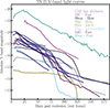 |
Fig. 16. V-band absolute magnitude light curves of the CSP fast-declining SN II subsample, together with the comparison literature SNe. |
SN 2006ai: Absolute magnitude light curves and the visual-wavelength spectral sequence of SN 2006ai are displayed in Fig. 17. The figure shows a few additional features common to many of the fast decliners that have not been noted above. After peak magnitude (which is well observed for SN 2006ai), this event displays a clear fast initial decline (s1) before settling onto the more slowly declining s2 (that is still clearly much quicker than e.g. SN 1999em in the figure). This clear s1–s2 break is observed in a number of other well-observed SNe II (both slow and fast decliners: SN 2004er, SN 2006Y, SN 2008M, SN 2008aw, SN 2008if, SN 2009N). SN 2006ai evolves quickly through the transition phase, arriving to the tail before +80 d: the overall time evolution of this event – together with many other of the fast decliners – is significantly faster than that of ‘normal’ slow decliners. The spectral sequence displayed in Fig. 17 shows the typical features of a SN II; however, comparing it to the slow-declining SN 2005J (Fig. 12), one observes that the Hα absorption component is very weak in SN 2006ai. Gutiérrez et al. (2014) indeed showed that higher-s2 SNe II generally display lower absorption to emission strengths of Hα (a/e) compared to the rest of the population. M22b constrains SN 2006ai to be an extremely energetic event (compared with the rest of the sample), with an explosion energy constrained to be 1.3 ± 0.08 foe – consistent with the fast evolution of the different light-curve phases.
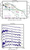 |
Fig. 17. Absolute and apparent magnitude uBgVri and YJH light curves (top) and visual-wavelength spectra (bottom) of SN 2006ai. The V-band absolute magnitude light curves of SN 1979C and SN 1999em are also displayed for comparison. |
SN 2007ab: Absolute magnitude light curves and the visual-wavelength spectral sequence of SN 2007ab are displayed in Fig. 18. SN 2007ab is the fastest decliner in the CSP sample, with an s2 of 3.3 ± 0.06 mag/100 d. It also has a relatively short OPTd of 70 ± 10 days. As Fig. 18 shows, SN 2007ab displays a very shallow transition from the plateau to tail phases – such a transition would have been undetectable if less photometry had been available. Unfortunately the first few weeks of transient evolution were missed and therefore it is unclear how bright this object was at maximum. SN 2007ab shows even weaker metal line formation than SN 2006ai, while its Hα feature is particularly strong. Hα50 is 9770 ± 510 km/s, significantly higher than the median sample value and higher than that of SN 2006ai. Hydrodynamical modelling in M22b constrains the explosion energy to be 1.2 ± 0.07 foe – twice the median sample value. Indeed, a common property of fast-declining SNe II appears to be their high estimated explosion energies (M22c).
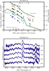 |
Fig. 18. Absolute and apparent magnitude uBgVri and YJH light curves (top) and visual-wavelength spectra (bottom) of SN 2007ab. The V-band absolute magnitude light curves of SN 1979C and SN 2014G are also displayed for comparison. |
SN 2008if: Absolute magnitude light curves and the visual-wavelength spectral sequence of SN 2008if are displayed in Fig. 19. SN 2008if is extremely well observed, both in photometry and spectroscopy. It shows a very similar light-curve morphology to SN 2006ai: a peak (most easily seen in NIR bands, as at bluer wavelengths the peak is earlier), followed by a steeper decline phase (s1), which then breaks to a slower decline (s2) and shows a shallow transition to the radioactive tail. With an OPTd of 76 ± 6 days, SN 2008if again shows a shorter plateau phase than the general SN II population. Figure 19 displays the high-cadence spectral sequence of SN 2008if, the features of which are typical for hydrogen-rich SNe II. However, one may again note the weak Hα absorption – as compared to SN 2005J (Fig. 12), a previous example of a slowly declining SN II. Once again SN 2008if is estimated (M22b) to have a relatively large explosion energy of 1.0 ± 0.06 foe (together with a low progenitor ZAMS mass of 10.1 ± 0.13 M⊙).
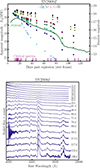 |
Fig. 19. Absolute and apparent magnitude uBgVri and YJH light curves (top) and visual-wavelength spectra (bottom) of SN 2008if. The V-band absolute magnitude light curve of SN 2014G is also displayed for comparison. |
SN 2006bl: Absolute magnitude light curves and the visual-wavelength spectral sequence of SN 2006bl are displayed in Fig. 20. As stated above, SN 2006bl is a clear fast decliner, with an s2 of 2.5 ± 0.06 mag/100 d; however, given that only three spectra were obtained it did not fall within the selection criteria for our fast-declining subsample. We highlight it here as it is one of the few CSP SNe II that one could claim shows a true classical IIL light-curve morphology. There is no clear break in the light curve defining any transition from a photospheric to tail phase. Also, unlike some of the fast decliners discussed above, SN 2006bl does not display any clear decline-rate break post peak (no clear s1 to s2 transition). It is also relatively bright at –18.2 ± 0.07 mag (median of –16.7 mag). The spectra that were obtained show strong and broad Hα emission (Fig. 20) with weak absorption (although the last spectrum is only at +29 d). Interestingly, modelling from M22b constrains SN 2006bl to have exploded with the highest explosion energy of the CSP-I sample (1.4 ± 0.08 foe) and to have also arisen from a relatively high initial mass progenitor (ZAMS mass of 15.5 ± 2.1 M⊙). However, the modelling for this event is not particularly well constrained, given that it is not possible to define the end of any plateau phase.
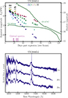 |
Fig. 20. Absolute and apparent magnitude uBgVri and YJH light curves (top) and visual-wavelength spectra (bottom) of SN 2006bl. The V-band absolute magnitude light curves of SN 1979C and SN 1999em are also displayed for comparison. |
5.3. A few peculiar SNe II
Finally, in this section we highlight and discuss the properties of a small number of non-standard SNe II that are either hard to classify in the context of the previous discussion, or that show some peculiarity that sets them apart from the rest of the CSP (and indeed literature) sample.
SN 2004dy: Absolute magnitude light curves and the visual-wavelength spectral sequence of SN 2004dy are displayed in Fig. 21. Unfortunately only a small amount of data were acquired for this event and thus strong conclusions on the origin of its peculiarity are not possible. The gVri light curves show a flat evolution for around two weeks before the light curve starts to decline in all bands. If this is interpreted as the end of a very short OPTd then such a light curve may be explained by the explosion of a progenitor with a small hydrogen envelope. Indeed, we measure an OPTd of 24 ± 6 days for SN 2004dy. However, this light-curve evolution does not match that of SNe IIb (see, e.g. Pessi et al. 2019), where the IIb class is thought to arise from progenitors with a low-mass hydrogen envelope at the epoch of explosion (inferred from their transition from hydrogen to helium line dominated spectra over the first few weeks post explosion; Filippenko 1988; Filippenko et al. 1993). This difference probably implies a difference in the pre-SN progenitor structure. The spectra (Fig. 21) are also not particularly constraining – they are quite noisy and end at +28 d. The strongest line is seen just short of 6000 Å, and may be due to sodium or helium. Hα is also observed. However given the weakness of this line and the other transient properties it is not clear whether SN 2004dy is a true hydrogen-rich SN II.
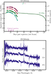 |
Fig. 21. Absolute and apparent magnitude uBgVri and YJH light curves (top) and visual-wavelength spectra (bottom) of SN 2004dy. The V-band absolute magnitude light curve of SN 1999gi is also displayed for comparison. |
SN 2006Y: Absolute magnitude light curves and the visual-wavelength spectral sequence of SN 2006Y are displayed in Fig. 22. Comparing to the fast decliners discussed in the previous subsection, SN 2006Y may be seen as an extreme version of SN 2006ai and SN 2008if. The event discussed here is a significant outlier in most observed properties of SNe II (see A14 and Gutiérrez et al. 2017a). The epoch of peak brightness was probably missed (but only by a few days), then an extremely fast initial decline (s1) is observed (significantly faster than in any other SN II in the sample). It shows a quite abrupt s1 to s2 transition and a well-defined plateau stage. This ends at only 46 ± 5 days post explosion (Table 1). This short OPTd probably implies that SN 2006Y came from a progenitor that had suffered significant envelope stripping prior to explosion (given that plateau length is associated with hydrogen envelope mass, see M22c). At the end of its OPTd, SN 2006Y displays a transition to a tail phase. The spectral sequence (Fig. 22) is affected by significant host H II region contamination. Strong Hα is observed that has a very weak or nonexistent absorption component. Its Fe50 is 5080 ± 550 km/s, significantly higher than the sample median (3940 km/s). No reasonable solution was found in fitting hydrodynamical models to the observations of SN 2006Y in M22b, owing to the short plateau phase. However, in M22c additional progenitor models were used where additional mass-loss was assumed during stellar evolution, producing pre-SN progenitors with much smaller hydrogen envelopes. The best-fit model was a progenitor with a 4.4 ± 0.36 M⊙ hydrogen envelope mass (compared to 7.1 M⊙ for the lowest hydrogen envelope fit to CSP-I SNe II using standard mass-loss values). In addition, M22c constrained the explosion energy to be 1.2 ± 0.2 foe and the ejected 56Ni mass to be 0.08 ± 0.004 M⊙. Thus, the main properties of SN 2006Y can be explained by a high-energy explosion of a progenitor with a low hydrogen envelope mass and significant ejection of radioactive material. We note that Hiramatsu et al. (2021) also concluded that a low hydrogen-envelope mass is required to model the data of SN 2006Y.
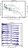 |
Fig. 22. Absolute and apparent magnitude uBgVri and YJH light curves (top) and visual-wavelength spectra (bottom) of SN 2006Y. The V-band absolute magnitude light curve of SN 2014G is also displayed for comparison. |
SN 2009A: Absolute magnitude light curves and the visual-wavelength spectral sequence of SN 2009A are displayed in Fig. 23. To our knowledge, this SN II displays a unique light curve and spectral evolution. The first photometry (uBgVri) was obtained just after 10 days post explosion and shows a very steep decline that is most pronounced in the bluer bands (a drop of around 1.5 mag in just over 10 days in B). The spectra obtained during this phase (Fig. 23) show strong and broad Hα and Hβ, with the Hα profile evolving quite quickly between +15 d and +19 d – the peak becomes sharper by the latter epoch. Between +25 and +33 d the decline halts (unfortunately, no spectra were obtained during this phase). Then, the light curve rises again by around a magnitude in 10 days. The next photometric epoch stays at almost the same brightness, and no more photometry was obtained. At the end of the observed light curve two additional spectra (taken only a day apart) show what seems to be a double P-Cygni Hα profile superimposed onto one another – probably implying two distinct line forming regions. The emission peak of Hα is blueshifted by ∼5500 km/s. Such blueshifts are a common feature of SNe II (see Anderson et al. 2014b). However, the velocity is extremely high compared to any other SN II. The narrower P-Cygni profile of Hα has an absorption component that is blueshifted by nearly 15 000 km/s at around +45 d. This is ∼6000 km/s faster than any other CSP SN II. In summary, SN 2009A shows a light curve evolution and spectral properties that are not observed in any other event in our sample, and that to our knowledge have not been observed in any other literature SN II. It is unclear what progenitor and explosion properties could produce such transient behaviour, and we encourage future modelling of this event.
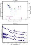 |
Fig. 23. Absolute and apparent magnitude uBgVri and YJH light curves (top) and visual-wavelength spectra (bottom) of SN 2009A. |
Other mentionable CSP SNe II: Before concluding, we very briefly discuss a few other CSP SNe II that do not appear to fall within the main observational parameter space of hydrogen-rich SNe II. As described above, a study of three SNe II was published by Rodríguez et al. (2020): SNe 2008bm, 2009aj and 2009au. Those three were named ‘luminous for their low expansion velocities’ SNe II in reference to them being outliers in the luminosity-velocity correlation used in the application of SNe II as distance indicators (see, e.g. Hamuy & Pinto 2002). That study concluded that the behaviour of these events can be explained by significant ejecta-CSM interaction18 that boosts the early luminosity and also decelerates the ejecta to produce low velocities. SN 2008bu is a fast decliner with an s2 of 2.4 ± 0.02 mag/100 d – but it was not part of the above subsample owing to a lack of sufficient spectral observations. This event shows an extremely short OPTd of only 44 ± 8 days. Similarly to SN 2006Y above, SN 2008bu was modelled by M22c using a progenitor with enhanced mass loss – to enable fitting to its short plateau phase. Finally, SN 2009ao displays a strange light curve that looks somewhat similar to that of SN 2004dy presented above. It has an OPTd of 42 ± 6 days, however it is unclear whether such a phase measurement is applicable here. Compared to SN 2004dy, SN 2009ao displays a standard spectral sequence (see Gutiérrez et al. 2017a). Given the lack of data after +60 d, it is unclear how to interpret this event.
6. Summary and future outlook
We have presented uBgVri optical and YJH NIR photometry for a total of 94 SNe II from two campaigns of the Carnegie Supernova Project (CSP-I and CSP-II). This low-redshift sample is characterised by being of high quality and cadence for the first ∼150 days post explosion. While most of the data have been quantitatively analysed and robustly modelled elsewhere, here we present the final photometry for widespread use, and have provided an analysis of the sample properties. A descriptive analysis was presented to summarise the CSP SN II sample and the SN II phenomenon in general, while we have additionally highlighted a number of standard and nonstandard SNe II that aid in understanding the diversity observed within hydrogen-rich SNe II.
With the advancement in survey detection and follow-up efficiency, the number of SNe classified as type II can now be counted in the thousands19. The number of well-observed nearby events with multiwavelength photometry is (with the current data release) around several hundred SNe II. Given the large samples of ‘standard’ SNe that are now available in the literature (SNe II as discussed here, but also SNe Ia and SE-SNe), SN science has started to focus on observing and understanding nonstandard explosions and/or to investigate observational parameter space previously unexplored (e.g. very early times within hours of explosion). Both of these avenues of research are being aided by the increased capabilities of surveys that enable a significant fraction of the observable sky to be scanned at a frequency of one day or less (see e.g. ASASSN, Shappee et al. 2014; Kochanek et al. 2017; ATLAS, Tonry et al. 2018; Smith et al. 2020; ZTF, Bellm et al. 2019; KMTNet, Afsariardchi et al. 2019). Such surveys also provide optical light curves of transients (down to their survey limits), meaning that the number of SNe with useable light curves increases rapidly each year. However, those light curves have usually at most two or three wavelength bands and thus only afford a first-order characterisation of transient behaviour. The number of events that will have spectral sequences is much lower owing to the expensive nature of spectroscopic observations. Thus, to enable the optimal science extraction from future SN II samples, a well-defined comparison and calibration sample is required. The current CSP SN II data release fulfils this requirement. Of particular importance for modelling SNe II to understand physical parameters of the explosions is the estimation of bolometric light curves. The u to H wavelength range of the CSP enables this sample to be used to calibrate lower-quality (in terms of wavelength coverage) photometry and obtain bolometric fluxes following the methodologies outlined by M22a20.
The coming years will welcome the arrival of another leap in survey capability with the Legacy Survey of Space and Time, LSST (LSST Science Collaboration 2009) to be undertaken by the Vera C. Rubin Observatory (together with a number of other upcoming facilities that will also change the transient landscape). LSST will provide multiwavelength optical light curves for many thousands of SNe II each year. These data will enable much larger population studies than currently possible. However, spectroscopy will be scarce, as will NIR photometry (as they would require separate follow-up campaigns). Thus, a full understanding of future statistical light-curve samples will only be possible by comparison to high-quality samples such as that presented in the current work (and other examples in the literature).
As discussed in the introduction, SNe II – and indeed the CSP sample – have been used to measure distances and have been proposed to be used to measure galaxy metallicities. The full potential future use of hydrogen-rich SNe in this direction, out to high redshift, will require that the high-redshift events are calibrated against nearby samples where high-quality light curves and spectra exist, such as the CSP SN II database.
The utility of precise photometry also requires accurate measurements of the transmission functions which define the natural photometric system. Transmission functions are crucial for k-corrections. Type II supernovae can have strong emission lines, which if they fall near the edge of a filter function, can introduce 0.1 mag or larger errors if the transmission function is not well calibrated.
Throughout this paper, we have reiterated the high-quality nature of this data set, implying it can be used to aid in investigating a number of astrophysical and cosmological questions. However, as suggested above, while the CSP SN II sample is of high quality in some important aspects, it does not cover the full observational parameter space of interest. The CSP-I sample (that makes up ∼3/4 of the full sample) has many events where follow-up was only started a week or more after explosion. During the time of that initial project, detecting SNe within a few days of explosion was relatively rare. Thus, the CSP SN II data presented cannot be used to probe the early time evolution of these hydrogen-rich events. Such observations are of significant interest as they can elucidate the progenitor structure – either the pre-SN radius or the extent and properties of any significant CSM close to the exploding star. Many projects are now concentrating on these early times as the scientific payoff is potentially significant. Indeed, the POISE collaboration (Precision Observations of Infant Supernova Explosions; Burns et al. 2021) is focusing on such observations.
While a number of studies have already been published using the current data (see Section 3.5), we envisage that additional valuable analysis is possible. M22a presented bolometric light curves that others may wish to model (together with the spectral velocities available from Gutiérrez et al. 2017a). The modelling achieved by M22b assumed standard single-star evolution parameters to create progenitors to explode and thus only sampled a constrained region of the possible progenitor parameter space. The results of M22b and M22c should be tested by independent modelling. The majority of the highlighted peculiar SNe discussed in the previous section warrant detailed modelling to understand which combinations of progenitor and explosion properties are able to produce such transients (of specific note is SN 2009A). There are also observational properties of SNe II that deserve additional attention and could be addressed using this sample. For example, to date CSP SN II studies have not analysed the shape and depth of the plateau to tail transition – this clearly changes significantly from one SN II to the next. It is unclear what physical parameters cause such diversity.
In conclusion, this paper has presented a legacy data set of SNe II: almost 100 SNe with u to H wavelength coverage and with high cadence and high-precision photometry from one week from explosion to more than 100 days later. The photometry is accompanied by optical and NIR spectroscopy previously analysed and released by Gutiérrez et al. (2017a) and Davis et al. (2019), respectively. This data set provides a baseline standard for future SN II samples, and has the potential to be critical for the future use of SNe II as astrophysical markers out to cosmological distances. While our understanding of SNe II has significantly advanced in the last few decades (e.g. constraints on progenitors, constraints on CSM surrounding those progenitors), there are still many uncertainties in the exact mapping from exploding progenitors to observed transients. Additional observations will continue to further our understanding of the SN II phenomenon, but data sets such as that presented here will provide the foundations on top of which future advances in our knowledge of the explosions of massive hydrogen-rich stars can be built.
Data availability
Photometry for local-sequence stars and for all SNe II presented in this paper are available at the CDS via anonymous ftp to cdsarc.cds.unistra.fr (http://cdsarc.u-strasbg.fr) or via https://cdsarc.cds.unistra.fr/viz-bin/cat/J/A+A/692/A95 and the same data can be downloaded from the CSP website: https://csp.obs.carnegiescience.edu/data. Figures of the optical and NIR apparent and absolute magnitude light curves of the CSP SN II sample can be found on Zenodo at the following link: https://zenodo.org/records/13743220. Finder charts for all SNe II in our sample can be found on Zenodo at the following link: https://zenodo.org/records/13743254. Tables listing important information on all SNe II in the CSP sample can be found on Zenodo at the following link: https://zenodo.org/records/13743303.
The optical spectral sequences of CSP-I SNe II were published by Gutiérrez et al. (2017a).
The release of the current dataset and those of other SN types published in previous works means that the CSP has attained its aim of establishing a fundamental data set of SNe. Data releases for CSP-I SNe Ia can be found in Krisciunas et al. (2017), Stripped-Envelope events (SE-SNe: type IIb, Ib and Ic) in Stritzinger et al. (2018), SNe IIn in Taddia et al. (2013), and data for two 1987A-like events in Taddia et al. (2012).
While the prior in the explosion epoch modelling of Martinez et al. (2022b) was defined to be within the observational explosion limits, it does not follow that the mean offset has to be close to zero. Additionally, in Martinez et al. (2020) such priors were relaxed (allowing explosion epochs outside the observational limits) and negligible changes were observed in the resulting explosion epochs.
The same data can also be downloaded from the CSP website: https://csp.obs.carnegiescience.edu/data
In A14 and Gutiérrez et al. (2017a) we also defined ‘Pd’ (‘plateau duration’) – the time from the s1-to-s2 inflection point until the end of OPTd. However, that parameter is harder to measure and thus we use OPTd here to provide a greater sample size for comparison.
ASASSN-15nx may be considered the only true SN IIL thus far observed if one uses a literal interpretation of the initial IIP, IIL classification scheme (Barbon et al. 1979).
The errors quoted on the physical parameters are statistical and are small due to the high quality of the observations of our sample. However, they do not include uncertainties arising from choices in standard stellar evolution modelling parameters. In addition, the asymmetric errors given in M22b are averaged here for presentation purposes.
Gutiérrez et al. (2017b) presented a weak anticorrelation between s2 and OPTd.
See the Transient Name Server, TNS, for lists of SN discoveries and classifications: https://www.wis-tns.org/
Acknowledgments
This project was supported by the U.S. National Science Foundation (NSF) under grants AST-0306969, AST-0607438, AST-1008343, AST-1613426, AST-1613455, and AST-1613472. The CSP-II was also supported in part by the Danish Agency for Science and Technology and Innovation through a Sapere Aude Level 2 grant. M.D.S. is funded in part by a research Project 1 grant from the Independent Research Fund Denmark (IRFD grant numbers 8021-00170B and 10.46540/2032-00022B) and by a VILLUM FONDEN Experiment (grant number 28021). S.G.G. acknowledges support by FCT under Project CRISP PTDC/FIS-AST-31546/2017 and FCT Project No. UIDB/00099/2020. CPG acknowledges financial support from the Secretary of Universities and Research (Government of Catalonia) and by the Horizon 2020 Research and Innovation Programme of the European Union under the Marie Skłodowska-Curie and the Beatriu de Pinós 2021 BP 00168 programme, from the Spanish Ministerio de Ciencia e Innovación (MCIN) and the Agencia Estatal de Investigación (AEI) 10.13039/501100011033 under the PID2023-151307NB-I00 HOSTFLOWS project, and the program Unidad de Excelencia María de Maeztu CEX2020-001058-M. N.B.S., K.K., D.D., and S.U. acknowledge the support of the Mitchell Institute for Fundamental Physics and Astronomy. They also acknowledge the Mitchell Foundation and Sheridan Lorenz for funding workshops at the Mitchell Cooks Branch Nature Preserve. C.A. is supported by NSF grants AST-1907570, AST-1908952, AST-1920392, and AST-1911074. L.M. acknowledges support from a CONICET fellowship and from grant UNRN PI2018 40B696. L.G. acknowledges financial support from the Spanish Ministerio de Ciencia e Innovación (MCIN), the Agencia Estatal de Investigación (AEI) 10.13039/501100011033, and the European Social Fund (ESF) “Investing in your future” under the 2019 Ramón y Cajal program RYC2019-027683-I and the PID2023-151307NB-I00 HOSTFLOWS project, and from Centro Superior de Investigaciones Científicas (CSIC) under the PIE project 20215AT016. C.G. is supported by a VILLUM FONDEN Young Investor Grant (project number 25501). P.H. acknowledges support by NSF grant AST-856-1715133. A.V.F. has received support from the UC Berkeley Miller Institute for Basic Research in Science (where he was a Miller Senior Fellow), the TABASGO foundation, the Christopher R. Redlich Fund, and many individual donors. F.F acknowledges National Agency of Research and Development’ (ANID) Millennium Science Initiative through grant IC12009, awarded to the Millennium Institute of Astrophysics, ANID BASAL grant Center of Mathematical Modelling AFP-170001, ACE210010, FB210005 and ANID BASAL grant center FB210003, and FONDECYT Regular 1200710. B.J.S. is supported by NSF grants AST-1908952, AST-1920392 and AST-1911074. This research has made use of the NASA/IPAC Extragalactic Database (NED) which is operated by the Jet Propulsion Laboratory, California Institute of Technology, under contract with the National Aeronautics and Space Administration. Software: NumPy (Van Der Walt et al. 2011), matplotlib (Hunter 2007), SNID (Blondin & Tonry 2007). Facilities:Magellan: Baade (IMACS imaging spectrograph, FourStar wide-field near-infrared camera, FIRE near-infrared echellette), Magellan: Clay (LDSS3 imaging spectrograph), Swope (SITe3 CCD imager, e2v 4K × 4K CCD imager), du Pont (Tek5 CCD imager, WFCCD imaging spectrograph, RetroCam near-infrared imager), Gemini:North (GNIRS near-infrared spectrograph), Gemini:South (FLAMINGOS2), La Silla-QUEST, CRTS, PTF, iPTF, OGLE, ASASSN, PS1, KISS, ISSP, MASTER, SMT.
References
- Afsariardchi, N., Moon, D.-S., Drout, M. R., et al. 2019, ApJ, 881, 22 [NASA ADS] [CrossRef] [Google Scholar]
- Anderson, J. P., González-Gaitán, S., Hamuy, M., et al. 2014a, ApJ, 786, 67 [Google Scholar]
- Anderson, J. P., Dessart, L., Gutierrez, C. P., et al. 2014b, MNRAS, 441, 671 [NASA ADS] [CrossRef] [Google Scholar]
- Anderson, J. P., Gutiérrez, C. P., Dessart, L., et al. 2016, A&A, 589, A110 [NASA ADS] [CrossRef] [EDP Sciences] [Google Scholar]
- Anderson, J. P., Dessart, L., Gutiérrez, C. P., et al. 2018, Nat. Astron., 2, 574 [NASA ADS] [CrossRef] [Google Scholar]
- Arcavi, I. 2017, in Hydrogen-Rich Core-Collapse Supernovae, eds. A. W. Alsabti, & P. Murdin, 239 [Google Scholar]
- Arcavi, I., Gal-Yam, A., Kasliwal, M. M., et al. 2010, ApJ, 721, 777 [NASA ADS] [CrossRef] [Google Scholar]
- Arcavi, I., Gal-Yam, A., Bradley Cenko, S., et al. 2012, ApJ, 756, L30 [NASA ADS] [CrossRef] [Google Scholar]
- Barbon, R., Ciatti, F., & Rosino, L. 1979, A&A, 72, 287 [Google Scholar]
- Barbon, R., Ciatti, F., & Rosino, L. 1982, A&A, 116, 35 [NASA ADS] [Google Scholar]
- Baron, E., Nugent, P. E., Branch, D., & Hauschildt, P. H. 2004, ApJ, 616, L91 [NASA ADS] [CrossRef] [Google Scholar]
- Bellm, E. C., Kulkarni, S. R., Graham, M. J., et al. 2019, PASP, 131, 018002 [Google Scholar]
- Bersten, M. C. 2013, ArXiv e-prints [arXiv:1303.0639] [Google Scholar]
- Bersten, M. C., Benvenuto, O., & Hamuy, M. 2011, ApJ, 729, 61 [NASA ADS] [CrossRef] [Google Scholar]
- Bersten, M. C., Folatelli, G., García, F., et al. 2018, Nature, 554, 497 [Google Scholar]
- Blondin, S., & Tonry, J. L. 2007, ApJ, 666, 1024 [NASA ADS] [CrossRef] [Google Scholar]
- Blondin, S., Modjaz, M., Kirshner, R., Challis, P., & Rines, K. 2007, Central Bureau Electronic Telegrams, 853, 1 [NASA ADS] [Google Scholar]
- Bose, S., Sutaria, F., Kumar, B., et al. 2015, ApJ, 806, 160 [Google Scholar]
- Bose, S., Dong, S., Kochanek, C. S., et al. 2018, ApJ, 862, 107 [NASA ADS] [CrossRef] [Google Scholar]
- Bruch, R. J., Gal-Yam, A., Schulze, S., et al. 2021, ApJ, 912, 46 [NASA ADS] [CrossRef] [Google Scholar]
- Burns, C., Hsiao, E., Suntzeff, N., et al. 2021, ATel, 14441, 1 [NASA ADS] [Google Scholar]
- Burrows, A., & Vartanyan, D. 2021, Nature, 589, 29 [CrossRef] [PubMed] [Google Scholar]
- Buta, R. J. 1982, PASP, 94, 578 [CrossRef] [Google Scholar]
- Cardelli, J. A., Clayton, G. C., & Mathis, J. S. 1989, ApJ, 345, 245 [Google Scholar]
- Chevalier, R. A. 1976, ApJ, 207, 872 [NASA ADS] [CrossRef] [Google Scholar]
- Contreras, C., Hamuy, M., Phillips, M. M., et al. 2010, AJ, 139, 519 [Google Scholar]
- Davies, B., & Beasor, E. R. 2018, MNRAS, 474, 2116 [NASA ADS] [CrossRef] [Google Scholar]
- Davies, B., & Beasor, E. R. 2020, MNRAS, 493, 468 [NASA ADS] [CrossRef] [Google Scholar]
- Davis, S., Hsiao, E. Y., Ashall, C., et al. 2019, ApJ, 887, 4 [NASA ADS] [CrossRef] [Google Scholar]
- de Jaeger, T., González-Gaitán, S., Anderson, J. P., et al. 2015, ApJ, 815, 121 [NASA ADS] [CrossRef] [Google Scholar]
- de Jaeger, T., Galbany, L., Filippenko, A. V., et al. 2017a, MNRAS, 472, 4233 [NASA ADS] [CrossRef] [Google Scholar]
- de Jaeger, T., González-Gaitán, S., Hamuy, M., et al. 2017b, ApJ, 835, 166 [NASA ADS] [CrossRef] [Google Scholar]
- de Jaeger, T., Anderson, J. P., Galbany, L., et al. 2018, MNRAS, 476, 4592 [NASA ADS] [CrossRef] [Google Scholar]
- de Jaeger, T., Zheng, W., Stahl, B. E., et al. 2019, MNRAS, 490, 2799 [NASA ADS] [CrossRef] [Google Scholar]
- de Jaeger, T., Galbany, L., González-Gaitán, S., et al. 2020, MNRAS, 495, 4860 [NASA ADS] [CrossRef] [Google Scholar]
- Dessart, L., & Hillier, D. J. 2019, A&A, 625, A9 [NASA ADS] [CrossRef] [EDP Sciences] [Google Scholar]
- Dessart, L., Blondin, S., Brown, P. J., et al. 2008, ApJ, 675, 644 [NASA ADS] [CrossRef] [Google Scholar]
- Dessart, L., Hillier, D. J., Waldman, R., & Livne, E. 2013, MNRAS, 433, 1745 [NASA ADS] [CrossRef] [Google Scholar]
- Dessart, L., Gutierrez, C. P., Hamuy, M., et al. 2014, MNRAS, 440, 1856 [NASA ADS] [CrossRef] [Google Scholar]
- de Vaucouleurs, G., de Vaucouleurs, A., Buta, R., Ables, H. D., & Hewitt, A. V. 1981, PASP, 93, 36 [NASA ADS] [CrossRef] [Google Scholar]
- Dhungana, G., Kehoe, R., Vinko, J., et al. 2016, ApJ, 822, 6 [NASA ADS] [CrossRef] [Google Scholar]
- Ensman, L., & Burrows, A. 1992, ApJ, 393, 742 [NASA ADS] [CrossRef] [Google Scholar]
- Falk, S. W., & Arnett, W. D. 1977, ApJS, 33, 515 [NASA ADS] [CrossRef] [Google Scholar]
- Faran, T., Poznanski, D., Filippenko, A. V., et al. 2014a, MNRAS, 445, 554 [NASA ADS] [CrossRef] [Google Scholar]
- Faran, T., Poznanski, D., Filippenko, A. V., et al. 2014b, MNRAS, 442, 844 [NASA ADS] [CrossRef] [Google Scholar]
- Faran, T., Goldfriend, T., Nakar, E., & Sari, R. 2019, ApJ, 879, 20 [NASA ADS] [CrossRef] [Google Scholar]
- Filippenko, A. V. 1988, AJ, 96, 1941 [CrossRef] [Google Scholar]
- Filippenko, A. V. 1997, ARA&A, 35, 309 [NASA ADS] [CrossRef] [Google Scholar]
- Filippenko, A. V., Matheson, T., Leibundgut, B., et al. 1993, IAU Circ., 5720, 1 [NASA ADS] [Google Scholar]
- Filippenko, A. V., Li, W. D., Treffers, R. R., & Modjaz, M. 2001, ASP Conf. Ser., 246, 121 [NASA ADS] [Google Scholar]
- Folatelli, G., Phillips, M. M., Burns, C. R., et al. 2010, AJ, 139, 120 [Google Scholar]
- Förster, F., Moriya, T. J., Maureira, J. C., et al. 2018, Nat. Astron., 2, 808 [CrossRef] [Google Scholar]
- Fryer, C. L. 2022, Int. J. Mod. Phys. D, 31, 2230005 [CrossRef] [Google Scholar]
- Galbany, L., Hamuy, M., Phillips, M. M., et al. 2016, AJ, 151, 33 [NASA ADS] [CrossRef] [Google Scholar]
- Gall, E. E. E., Kotak, R., Leibundgut, B., et al. 2016, A&A, 592, A129 [NASA ADS] [CrossRef] [EDP Sciences] [Google Scholar]
- Gall, E. E. E., Kotak, R., Leibundgut, B., et al. 2018, A&A, 611, A25 [NASA ADS] [CrossRef] [EDP Sciences] [Google Scholar]
- Garnavich, P. M., Tucker, B. E., Rest, A., et al. 2016, ApJ, 820, 23 [NASA ADS] [CrossRef] [Google Scholar]
- Gezari, S., Jones, D. O., Sanders, N. E., et al. 2015, ApJ, 804, 28 [NASA ADS] [CrossRef] [Google Scholar]
- González-Gaitán, S., Tominaga, N., Molina, J., et al. 2015, MNRAS, 451, 2212 [CrossRef] [Google Scholar]
- Grassberg, E. K., Imshennik, V. S., & Nadyozhin, D. K. 1971, Ap&SS, 10, 28 [Google Scholar]
- Gutiérrez, C. P., Anderson, J. P., Hamuy, M., et al. 2014, ApJ, 786, L15 [CrossRef] [Google Scholar]
- Gutiérrez, C. P., Anderson, J. P., Hamuy, M., et al. 2017a, ApJ, 850, 89 [CrossRef] [Google Scholar]
- Gutiérrez, C. P., Anderson, J. P., Hamuy, M., et al. 2017b, ApJ, 850, 90 [CrossRef] [Google Scholar]
- Gutiérrez, C. P., Anderson, J. P., Sullivan, M., et al. 2018, MNRAS, 479, 3232 [CrossRef] [Google Scholar]
- Hakobyan, A. A., Adibekyan, V. Z., Aramyan, L. S., et al. 2012, A&A, 544, A81 [NASA ADS] [CrossRef] [EDP Sciences] [Google Scholar]
- Hamuy, M. A. 2001, PhD Thesis, University of Arizona, USA [Google Scholar]
- Hamuy, M., & Pinto, P. A. 2002, ApJ, 566, L63 [NASA ADS] [CrossRef] [Google Scholar]
- Hamuy, M., Pinto, P. A., Maza, J., et al. 2001, ApJ, 558, 615 [NASA ADS] [CrossRef] [Google Scholar]
- Hamuy, M., Folatelli, G., Morrell, N. I., et al. 2006, PASP, 118, 2 [NASA ADS] [CrossRef] [Google Scholar]
- Hicken, M., Friedman, A.S., Challis, P., et al. 2017,MNRAS, submitted [arXiv:1706.01030] [Google Scholar]
- Hillier, D. J., & Dessart, L. 2019, A&A, 631, A8 [NASA ADS] [CrossRef] [EDP Sciences] [Google Scholar]
- Hiramatsu, D., Howell, D. A., Moriya, T. J., et al. 2021, ApJ, 913, 55 [CrossRef] [Google Scholar]
- Hoyle, F. 1954, ApJS, 1, 121 [NASA ADS] [CrossRef] [Google Scholar]
- Hsiao, E. Y., Phillips, M. M., Marion, G. H., et al. 2019, PASP, 131, 014002 [NASA ADS] [CrossRef] [Google Scholar]
- Huang, F., Wang, X., Zhang, J., et al. 2015, ApJ, 807, 59 [Google Scholar]
- Hunter, J. D. 2007, Comput. Sci. Eng., 9, 90 [NASA ADS] [CrossRef] [Google Scholar]
- Inserra, C., Pastorello, A., Turatto, M., et al. 2013, A&A, 555, A142 [NASA ADS] [CrossRef] [EDP Sciences] [Google Scholar]
- Janka, H. T. 2017, in Handbook of Supernovae, eds. A. W. Alsabti, & P. Murdin, 1095 [CrossRef] [Google Scholar]
- Khazov, D., Yaron, O., Gal-Yam, A., et al. 2016, ApJ, 818, 3 [CrossRef] [Google Scholar]
- Kirshner, R. P., & Kwan, J. 1974, ApJ, 193, 27 [NASA ADS] [CrossRef] [Google Scholar]
- Kochanek, C. S., Beacom, J. F., Kistler, M. D., et al. 2008, ApJ, 684, 1336 [NASA ADS] [CrossRef] [Google Scholar]
- Kochanek, C. S., Shappee, B. J., Stanek, K. Z., et al. 2017, PASP, 129, 104502 [Google Scholar]
- Kozyreva, A., Nakar, E., & Waldman, R. 2019, MNRAS, 483, 1211 [NASA ADS] [CrossRef] [Google Scholar]
- Krisciunas, K., Contreras, C., Burns, C. R., et al. 2017, AJ, 154, 211 [NASA ADS] [CrossRef] [Google Scholar]
- Landolt, A. U. 1992, AJ, 104, 340 [Google Scholar]
- Leonard, D. C., Filippenko, A. V., Li, W., et al. 2002a, AJ, 124, 2490 [NASA ADS] [CrossRef] [Google Scholar]
- Leonard, D. C., Kanbur, S. M., Ngeow, C. C., Tanvir, N. R., et al. 2002b, PASP, 114, 35 [NASA ADS] [CrossRef] [Google Scholar]
- Levesque, E. M., Massey, P., Olsen, K. A. G., et al. 2005, ApJ, 628, 973 [Google Scholar]
- Li, W., Leaman, J., Chornock, R., et al. 2011, MNRAS, 412, 1441 [NASA ADS] [CrossRef] [Google Scholar]
- Limongi, M., & Chieffi, A. 2018, ApJS, 237, 13 [NASA ADS] [CrossRef] [Google Scholar]
- LSST Science Collaboration (Abell, P. A., et al.) 2009, ArXiv e-prints [arXiv:0912.0201] [Google Scholar]
- Martinez, L., Bersten, M. C., Anderson, J. P., et al. 2020, A&A, 642, A143 [NASA ADS] [CrossRef] [EDP Sciences] [Google Scholar]
- Martinez, L., Bersten, M. C., Anderson, J. P., et al. 2022a, A&A, 660, A40 [NASA ADS] [CrossRef] [EDP Sciences] [Google Scholar]
- Martinez, L., Bersten, M. C., Anderson, J. P., et al. 2022b, A&A, 660, A41 [NASA ADS] [CrossRef] [EDP Sciences] [Google Scholar]
- Martinez, L., Anderson, J. P., Bersten, M. C., et al. 2022c, A&A, 660, A42 [NASA ADS] [CrossRef] [EDP Sciences] [Google Scholar]
- Matsuura, M., Dwek, E., Barlow, M. J., et al. 2015, ApJ, 800, 50 [NASA ADS] [CrossRef] [Google Scholar]
- Mauerhan, J. C., Van Dyk, S. D., Johansson, J., et al. 2017, ApJ, 834, 118 [Google Scholar]
- Maza, J., & van den Bergh, S. 1976, ApJ, 204, 519 [NASA ADS] [CrossRef] [Google Scholar]
- Minkowski, R. 1941, PASP, 53, 224 [NASA ADS] [CrossRef] [Google Scholar]
- Modjaz, M., Gutiérrez, C. P., & Arcavi, I. 2019, Nat. Astron., 3, 717 [NASA ADS] [CrossRef] [Google Scholar]
- Moriya, T., Tominaga, N., Blinnikov, S. I., Baklanov, P. V., & Sorokina, E. I. 2011, MNRAS, 415, 199 [NASA ADS] [CrossRef] [Google Scholar]
- Morozova, V., Piro, A. L., & Valenti, S. 2017, ApJ, 838, 28 [NASA ADS] [CrossRef] [Google Scholar]
- Morozova, V., Piro, A. L., & Valenti, S. 2018, ApJ, 858, 15 [Google Scholar]
- Pastorello, A., Baron, E., Branch, D., et al. 2005, MNRAS, 360, 950 [CrossRef] [Google Scholar]
- Pastorello, A., Sauer, D., Taubenberger, S., et al. 2006, MNRAS, 370, 1752 [NASA ADS] [CrossRef] [Google Scholar]
- Patat, F., Barbon, R., Cappellaro, E., & Turatto, M. 1994, A&A, 282, 731 [NASA ADS] [Google Scholar]
- Pejcha, O. 2020, Reviews in Frontiers of Modern Astrophysics; From Space Debris to Cosmology, 189 [CrossRef] [Google Scholar]
- Persson, S. E., Murphy, D. C., Krzeminski, W., Roth, M., & Rieke, M. J. 1998, AJ, 116, 2475 [NASA ADS] [CrossRef] [Google Scholar]
- Persson, S. E., Murphy, D. C., Smee, S., et al. 2013, PASP, 125, 654 [NASA ADS] [CrossRef] [Google Scholar]
- Pessi, P. J., Folatelli, G., Anderson, J. P., et al. 2019, MNRAS, 488, 4239 [NASA ADS] [CrossRef] [Google Scholar]
- Pessi, P. J., Anderson, J. P., Folatelli, G., et al. 2023, MNRAS, 523, 5315 [NASA ADS] [CrossRef] [Google Scholar]
- Phillips, M. M., Contreras, C., Hsiao, E. Y., et al. 2019, PASP, 131, 014001 [Google Scholar]
- Pskovskii, Y. P. 1967, Sov. Astron., 11, 63 [NASA ADS] [Google Scholar]
- Reynolds, T. M., Fraser, M., Mattila, S., et al. 2020, MNRAS, 493, 1761 [NASA ADS] [CrossRef] [Google Scholar]
- Richardson, D., Branch, D., Casebeer, D., et al. 2002, AJ, 123, 745 [NASA ADS] [CrossRef] [Google Scholar]
- Rodríguez, Ó., Clocchiatti, A., & Hamuy, M. 2014, AJ, 148, 107 [CrossRef] [Google Scholar]
- Rodríguez, Ó., Pignata, G., Hamuy, M., et al. 2019, MNRAS, 483, 5459 [CrossRef] [Google Scholar]
- Rodríguez, Ó., Pignata, G., Anderson, J. P., et al. 2020, MNRAS, 494, 5882 [CrossRef] [Google Scholar]
- Rubin, A., & Gal-Yam, A. 2016, ApJ, 828, 111 [NASA ADS] [CrossRef] [Google Scholar]
- Rubin, A., Gal-Yam, A., De Cia, A., et al. 2016, ApJ, 820, 33 [NASA ADS] [CrossRef] [Google Scholar]
- Sanders, N. E., Soderberg, A. M., Gezari, S., et al. 2015, ApJ, 799, 208 [NASA ADS] [CrossRef] [Google Scholar]
- Schawinski, K., Justham, S., Wolf, C., et al. 2008, Science, 321, 223 [NASA ADS] [CrossRef] [Google Scholar]
- Schlafly, E. F., & Finkbeiner, D. P. 2011, ApJ, 737, 103 [Google Scholar]
- Schmidt, B. P., Kirshner, R. P., Eastman, R. G., et al. 1994, ApJ, 432, 42 [NASA ADS] [CrossRef] [Google Scholar]
- Schwartz, G. 1978, Ann. Statist., 6, 461 [NASA ADS] [Google Scholar]
- Scott, S., Nicholl, M., Blanchard, P., Gomez, S., & Berger, E. 2019, ApJ, 870, L16 [NASA ADS] [CrossRef] [Google Scholar]
- Shappee, B. J., Prieto, J. L., Grupe, D., et al. 2014, ApJ, 788, 48 [Google Scholar]
- Smartt, S. J. 2015, PASA, 32, e016 [NASA ADS] [CrossRef] [Google Scholar]
- Smartt, S. J., Maund, J. R., Hendry, M. A., et al. 2004, Science, 303, 499 [NASA ADS] [CrossRef] [Google Scholar]
- Smartt, S. J., Eldridge, J. J., Crockett, R. M., & Maund, J. R. 2009, MNRAS, 395, 1409 [CrossRef] [Google Scholar]
- Smith, J. A., Tucker, D. L., Kent, S., et al. 2002, AJ, 123, 2121 [NASA ADS] [CrossRef] [Google Scholar]
- Smith, K. W., Smartt, S. J., Young, D. R., et al. 2020, PASP, 132, 085002 [Google Scholar]
- Soderberg, A. M., Berger, E., Page, K. L., et al. 2008, Nature, 453, 469 [NASA ADS] [CrossRef] [Google Scholar]
- Soker, N. 2019, Res. Astron. Astrophys., 19, 095 [Google Scholar]
- Spiro, S., Pastorello, A., Pumo, M. L., et al. 2014,MNRAS, submitted [arXiv:1401.5426] [Google Scholar]
- Stritzinger, M. D., Phillips, M. M., Boldt, L. N., et al. 2011, AJ, 142, 156 [Google Scholar]
- Stritzinger, M., Taddia, F., Fransson, C., et al. 2012, ApJ, 756, 173 [NASA ADS] [CrossRef] [Google Scholar]
- Stritzinger, M. D., Anderson, J. P., Contreras, C., et al. 2018, A&A, 609, A134 [NASA ADS] [CrossRef] [EDP Sciences] [Google Scholar]
- Suntzeff, N. B., Phillips, M. M., Elias, J. H., Depoy, D. L., & Walker, A. R. 1992, ApJ, 384, L33 [NASA ADS] [CrossRef] [Google Scholar]
- Taddia, F., Stritzinger, M. D., Sollerman, J., et al. 2012, A&A, 537, A140 [NASA ADS] [CrossRef] [EDP Sciences] [Google Scholar]
- Taddia, F., Stritzinger, M. D., Sollerman, J., et al. 2013, A&A, 555, A10 [NASA ADS] [CrossRef] [EDP Sciences] [Google Scholar]
- Taddia, F., Moquist, P., Sollerman, J., et al. 2016, A&A, 587, L7 [NASA ADS] [CrossRef] [EDP Sciences] [Google Scholar]
- Takáts, K., Stoica, R. S., Martínez, V. J., et al. 2014, MNRAS, 438, 368 [CrossRef] [Google Scholar]
- Terreran, G., Jerkstrand, A., Benetti, S., et al. 2016, MNRAS, 462, 137 [Google Scholar]
- Tominaga, N., Morokuma, T., Tanaka, M., et al. 2019, ApJ, 885, 13 [NASA ADS] [CrossRef] [Google Scholar]
- Tonry, J. L., Denneau, L., Heinze, A. N., et al. 2018, PASP, 130, 064505 [Google Scholar]
- Utrobin, V. P. 2007, A&A, 461, 233 [NASA ADS] [CrossRef] [EDP Sciences] [Google Scholar]
- Valenti, S., Sand, D., Pastorello, A., et al. 2014, MNRAS, 438, L101 [Google Scholar]
- Valenti, S., Sand, D., Stritzinger, M., et al. 2015, MNRAS, 448, 2608 [NASA ADS] [CrossRef] [Google Scholar]
- Valenti, S., Howell, D. A., Stritzinger, M. D., et al. 2016, MNRAS, 459, 3939 [NASA ADS] [CrossRef] [Google Scholar]
- Vallely, P. J., Kochanek, C. S., Stanek, K. Z., Fausnaugh, M., & Shappee, B. J. 2021, MNRAS, 500, 5639 [Google Scholar]
- Van Der Walt, S., Colbert, S. C., & Varoquaux, G. 2011, Comput. Sci. Eng., 13, 22 [Google Scholar]
- Van Dyk, S. D., Li, W., & Filippenko, A. V. 2003, PASP, 115, 1289 [NASA ADS] [CrossRef] [Google Scholar]
- Walmswell, J. J., & Eldridge, J. J. 2012, MNRAS, 419, 2054 [CrossRef] [Google Scholar]
- Waxman, E., & Katz, B. 2017, in Shock Breakout Theory, eds. A. W. Alsabti, & P. Murdin, 967 [Google Scholar]
- Yaron, O., Perley, D. A., Gal-Yam, A., et al. 2017, ArXiv e-prints [arXiv:1701.02596] [Google Scholar]
- Yoon, S.-C., & Cantiello, M. 2010, ApJ, 717, L62 [NASA ADS] [CrossRef] [Google Scholar]
- Young, T. R., & Branch, D. 1989, ApJ, 342, L79 [NASA ADS] [CrossRef] [Google Scholar]
Appendix A: Additional tables
Optical standard local sequence photometry (mag) for SN 2007oc.
NIR standard local sequence photometry (mag) for SN 2007oc.
Natural system optical photometry (mag) of SN 2007oc.
Natural system NIR photometry (mag) of SN 2007oc.
Appendix B: Updated data release for SNe IIn and SN 1987A-like events from CSP-I
Photometry (and spectroscopy) for five SNe IIn were released by Taddia et al. (2013) and for two SNe IIn by Stritzinger et al. (2012). The full sample of CSP-I SNe IIn consists of SNe 2005ip, 2005kj, 2006aa, 2006bo, 2006jd, 2006qq, 2008fq. In addition, data were released for two SN 1987A-like SNe II by Taddia et al. (2012): SNe 2006V and 2006au. During the subsequent years a number of small iterative changes were made to the CSP reduction and calibration procedures meaning that new updated photometry for these SNe is available in electronic, machine-readable format from the CDS, and can also be downloaded from the CSP website: https://csp.obs.carnegiescience.edu/data. These changes are very minor, and thus do not affect the results or conclusions published by the above works.
All Tables
All Figures
|
Fig. 1. Optical wavelength light curves of an example SN II together with the labelling of the different light curve phases. The distinct shaded regions are used to define where different physical processes dominate the luminosity of SNe II (see details in text). The generic naming scheme used in the literature to label these phases is given, together with observational parameters used to characterise those phases in brackets (from A14 and Gutiérrez et al. 2017b). It should be noted that phase boundaries are not necessarily well defined – they change between different SNe II, and are shown here as distinct abrupt changes for visualisation purposes. (While ‘SBO’ – shock breakout – is labelled on this plot and discussed in the text, it is not observed for this example SN II, nor for any other event in our sample). |
| In the text | |
|
Fig. 2. Redshift distributions of the CSP-I and CSP-II SN II samples. The number of events in each subsample is given in brackets. |
| In the text | |
|
Fig. 3. Number of optical (uBgVri) and NIR (YJH) photometric data points per SN for the CSP-I and CSP-II SN II samples. The number of events in each subsample is given in brackets. |
| In the text | |
|
Fig. 4. Distribution of the epochs of the earliest optical and NIR photometry obtained (with respect to explosion epoch) for each SN in our sample. The number of events in each subsample is given in brackets. The inset shows a zoom into the first 13 days post explosion. |
| In the text | |
|
Fig. 5. Distribution of the epochs of the latest optical and NIR photometry obtained (with respect to explosion epoch) for each SN in our sample. The number of events in each subsample is given in brackets. |
| In the text | |
|
Fig. 6. Finder chart of SN 2007oc with the SN position marked with a red cross, while optical local sequence stars are marked with blue circles. (Such finder charts for all SNe II in our sample can be found on Zenodo through the link in the data availability section). |
| In the text | |
|
Fig. 7. uBgVri and YJH apparent and absolute magnitude light curves of SN 2007oc plotted relative to the explosion epoch. Epochs when visual-wavelength spectra were obtained are indicated on the abscissa. (Such light curves for all SNe II in our sample can be found on Zenodo through the link in the data availability section.) |
| In the text | |
|
Fig. 8. V-band s2 distribution for the CSP and comparison samples. The comparison sample values are shown as ticks on the abscissa. |
| In the text | |
|
Fig. 9. OPTd plateau duration distribution measured in the V band for the CSP and comparison samples. The comparison-sample values are shown as ticks on the abscissa. (ASASSN-15nx is not shown here as it was not possible to define the end of any plateau phase – there is no discernible break to the post maximum decline rate out to late times). |
| In the text | |
|
Fig. 10. uViH absolute magnitude light curves of CSP SNe II. Individual photometric points have been joined by lines to provide a visualisation of the different light curve morphologies observed at different wavelengths. |
| In the text | |
|
Fig. 11. Absolute and apparent magnitude uBgVri and YJH light curves (top) and visual-wavelength spectra (bottom) of SN 2004fx. The V-band absolute magnitude light curves of SN 1999em and SN 2005cs are also displayed for comparison. |
| In the text | |
|
Fig. 12. Absolute and apparent magnitude uBgVri and YJH light curves (top) and visual-wavelength spectra (bottom) of SN 2005J. The V-band absolute magnitude light curve of SN 1999em is also displayed for comparison. |
| In the text | |
|
Fig. 13. Absolute and apparent magnitude uBgVri and YJH light curves (top) and visual-wavelength spectra (bottom) of SN 2006bc. The V-band absolute magnitude light curve of SN 2005cs is also displayed for comparison. |
| In the text | |
|
Fig. 14. Absolute and apparent magnitude uBgVri and YJH light curves (top) and visual-wavelength spectra (bottom) of SN 2008ag. The V-band absolute magnitude light curve of SN 1999em is also displayed for comparison. |
| In the text | |
|
Fig. 15. Absolute and apparent magnitude uBgVri and YJH light curves (top) and NIR wavelength spectroscopy (bottom) of ASASSN-15bb. The V-band absolute magnitude light curve of SN 1999gi is also displayed for comparison. |
| In the text | |
|
Fig. 16. V-band absolute magnitude light curves of the CSP fast-declining SN II subsample, together with the comparison literature SNe. |
| In the text | |
|
Fig. 17. Absolute and apparent magnitude uBgVri and YJH light curves (top) and visual-wavelength spectra (bottom) of SN 2006ai. The V-band absolute magnitude light curves of SN 1979C and SN 1999em are also displayed for comparison. |
| In the text | |
|
Fig. 18. Absolute and apparent magnitude uBgVri and YJH light curves (top) and visual-wavelength spectra (bottom) of SN 2007ab. The V-band absolute magnitude light curves of SN 1979C and SN 2014G are also displayed for comparison. |
| In the text | |
|
Fig. 19. Absolute and apparent magnitude uBgVri and YJH light curves (top) and visual-wavelength spectra (bottom) of SN 2008if. The V-band absolute magnitude light curve of SN 2014G is also displayed for comparison. |
| In the text | |
|
Fig. 20. Absolute and apparent magnitude uBgVri and YJH light curves (top) and visual-wavelength spectra (bottom) of SN 2006bl. The V-band absolute magnitude light curves of SN 1979C and SN 1999em are also displayed for comparison. |
| In the text | |
|
Fig. 21. Absolute and apparent magnitude uBgVri and YJH light curves (top) and visual-wavelength spectra (bottom) of SN 2004dy. The V-band absolute magnitude light curve of SN 1999gi is also displayed for comparison. |
| In the text | |
|
Fig. 22. Absolute and apparent magnitude uBgVri and YJH light curves (top) and visual-wavelength spectra (bottom) of SN 2006Y. The V-band absolute magnitude light curve of SN 2014G is also displayed for comparison. |
| In the text | |
|
Fig. 23. Absolute and apparent magnitude uBgVri and YJH light curves (top) and visual-wavelength spectra (bottom) of SN 2009A. |
| In the text | |
Current usage metrics show cumulative count of Article Views (full-text article views including HTML views, PDF and ePub downloads, according to the available data) and Abstracts Views on Vision4Press platform.
Data correspond to usage on the plateform after 2015. The current usage metrics is available 48-96 hours after online publication and is updated daily on week days.
Initial download of the metrics may take a while.