| Issue |
A&A
Volume 669, January 2023
|
|
|---|---|---|
| Article Number | A30 | |
| Number of page(s) | 11 | |
| Section | Stellar structure and evolution | |
| DOI | https://doi.org/10.1051/0004-6361/202244328 | |
| Published online | 03 January 2023 | |
Broadband study and the discovery of pulsations from the Be/X-ray binary eRASSU J052914.9−662446 in the Large Magellanic Cloud
1
Max-Planck-Institut für extraterrestrische Physik, Gießenbachstraße 1, 85748 Garching, Germany
e-mail: This email address is being protected from spambots. You need JavaScript enabled to view it.
2
South African Astronomical Observatory, PO Box 9 Observatory Rd, Observatory 7935, South Africa
3
Department of Astronomy, University of Cape Town, Private Bag X3, Rondebosch 7701, South Africa
4
Astronomical Observatory, University of Warsaw, Al. Ujazdowskie 4, 00-478 Warszawa, Poland
5
Institut für Astronomie und Astrophysik, Sand 1, 72076 Tübingen, Germany
6
Dr. Karl Remeis-Observatory and Erlangen Centre for Astroparticle Physics, Friedrich-Alexander-Universitẗ Erlangen-Nürnberg, Sternwartstr. 7, 96049 Bamberg, Germany
7
Department of Physics and Astronomy, Howard University, Washington, DC 20059, USA
8
CRESST/Code 661 Astroparticle Physics Laboratory, NASA Goddard Space Flight Center, Greenbelt Rd., MD 20771, USA
9
Universities Space Research Association, Huntsville, USA
10
Université de Strasbourg, CNRS, Observatoire astronomique de Strasbourg, UMR 7550, 67000 Strasbourg, France
Received:
23
June
2022
Accepted:
31
August
2022
Abstract
Context. The Magellanic Clouds are our nearest star-forming galaxies. While the population of high-mass X-ray binaries (HMXBs) in the Small Magellanic Cloud is relatively well studied, our knowledge about the Large Magellanic Cloud (LMC) is far from complete given its large angular extent and the insufficient coverage with X-ray observations.
Aims. We conducted a search for new HMXBs in the LMC using data from eROSITA, the soft X-ray instrument on board the Spektrum-Roentgen-Gamma satellite.
Methods. After confirming the nature of eRASSU J052914.9−662446 as a hard X-ray source that is positionally coincident with an early-type star, we followed it up with optical spectroscopic observations from the South African Large Telescope (SALT) and a dedicated NuSTAR observation.
Results. We study the broadband timing and spectral behaviour of the newly discovered HMXB eRASSU J052914.9−662446 through eROSITA, Swift, and NuSTAR data in X-rays and the Optical Gravitational Lensing Experiment (OGLE) and SALT RSS data at the optical wavelength. We report the detection of a spin period at 1412 s and suggest that the orbital period of the system is ∼151 days. We thereby establish that eRASSU J052914.9−662446 is an accreting pulsar. Furthermore, through optical spectroscopic observations and the detection of Hα emission, the source is identified as a Be X-ray binary pulsar in the LMC. We also investigated the variability of the source in the optical and X-ray regime over the past decades and provide estimates of the possible magnetic field strength of the neutron star.
Key words: Magellanic Clouds / X-rays: binaries / stars: emission-line / Be / stars: neutron
© The Authors 2023
 Open Access article, published by EDP Sciences, under the terms of the Creative Commons Attribution License (https://creativecommons.org/licenses/by/4.0), which permits unrestricted use, distribution, and reproduction in any medium, provided the original work is properly cited.
This article is published in open access under the Subscribe-to-Open model.
Open access funding provided by Max Planck Society.
1. Introduction
The Magellanic Clouds are our nearest star-forming galaxies. The current global star formation rates (SFR) are 0.021–0.05 M⊙ yr−1 and 0.068–0.161 M⊙ yr−1 for the Small Magellanic Cloud (SMC) and the Large Magellanic Cloud (LMC), respectively (For et al. 2018). The SMC in particular is known to host a large population of Be X-ray binaries (BeXRBs), which shows through a peak in the star formation activity between 25–40 Myr ago (Haberl & Sturm 2016; Antoniou & Zezas 2016). The high-mass X-ray binary (HMXB) population in the LMC is attributed to a star formation event at a slightly earlier epoch, and the formation efficiency of HMXBs in the LMC is also indicated to be lower than in the SMC (Antoniou & Zezas 2016). This information, however, is far from complete because of the large angular extent and insufficient coverage of the LMC by X-ray observations, which implies that only a part of the XRB population is known so far.
Our observational knowledge of the X-ray population of the Magellanic Clouds improved drastically with the launch of eROSITA, the soft X-ray instrument on board the Spektrum-Roentgen-Gamma (SRG) mission (Predehl et al. 2021), which surveyed the X-ray sky in an energy range of 0.2–8 keV between December 2019 and February 2022. This has led to the discovery of a number of new HMXBs, and to the detection of pulsations from previous candidate HMXBs. These detections confirmed their nature as neutron star X-ray binary systems (see e.g., Haberl et al. 2020, 2022a, 2021; Maitra et al. 2020a,b, 2021; Carpano et al. 2022).
eRASSU J052914.9−662446 was discovered during the course of the first eROSITA all-sky survey (eRASS1) as a new BeXRB in the LMC (Maitra et al. 2020a). Follow-up with the NuSTAR observatory through an unanticipated target of opportunity (ToO) observation revealed coherent pulsations from the source at 1412 s and confirmed its nature as a neutron star BeXRB (Maitra et al. 2020b). In this paper we report the X-ray broadband and multi-wavelength characteristics of eRASSU J052914.9−662446.
We describe the X-ray observations of eRASSU J052914.9−662446 using eROSITA all-sky survey, Swift, and NuSTAR data, and optical observations from the Optical Gravitational Lensing Experiment (OGLE; Udalski et al. 2008, 2015) and the Southern African Large Telescope (SALT; Buckley et al. 2006) in Sect. 2. In Sect. 3 we present the identification of the optical counterpart, search for X-ray variability and pulsations, and describe the broadband timing and spectral analysis with eROSITA and NuSTAR data. We report the optical long-term monitoring recorded by the OGLE (Sect. 3.6), and present the optical spectrum obtained with the SALT (Sect. 3.7). We discuss the results in Sect. 4 and provide the conclusions in Sect. 5.
2. Observations and data reduction
2.1. eROSITA
eRASSU J052914.9−662446 was discovered as a new bright and hard X-ray source after it was scanned for several weeks during eRASS1, performed by the eROSITA instrument on board the Russian/German Spektrum-Roentgen-Gamma (SRG) mission. Until the end of 2021, eROSITA scanned the source during five epochs in the energy range of 0.2–8 keV, as summarised in Table 1. The source was detected in all the epochs. To analyse the data, we used the eROSITA Standard Analysis Software System (eSASS version eSASSusers_201009;Brunner et al. 2022).
eROSITA observations of eRASSU J052914.9−662446.
We extracted eROSITA light curves and spectra using the eSASS task srctool following Maitra et al. (2021) and Haberl et al. (2022a). The source events were extracted using a circular region with a radius of 35″, and background events were extracted using a circle with a larger radius from a nearby source-free region. Events from all valid pixel patterns (PATTERN=15) were selected. For the spectral analysis, we combined the data from the five telescope modules (TM) with on-chip filter cameras into a single spectrum (TM 1–4 and 6). TM5 and TM7 were not used for spectroscopy because no reliable energy calibration is available so far due to an optical light leak that was discovered soon after the start of the CalPV phase (Predehl et al. 2021). The spectra were binned to achieve a minimum of one count per spectral bin to allow the use of Cash statistics (Cash 1979). The light curves were created using all seven cameras and by applying a cut in the fractional exposure of 0.15. Fractional exposure is a dimensionless quantity that corresponds to the product of the fractional collecting area and the fractional temporal coverage that overlaps with the time bin.
2.2. Swift
After its discovery with eROSITA, eRASSU J052914.9−662446 was followed up using the X-ray telescope (XRT; Gehrels et al. 2004; Burrows et al. 2005) on the Neil Gehrels Swift observatory on 2020 March 30 (MJD 58938.57–58938.98, OBSID 00013298003) with a 2.3 ks exposure. The Swift/XRT data were analysed following the Swift data analysis guide1 (Evans et al. 2007). Source detection was performed using a sliding-cell detection algorithm implemented by XIMAGE and sosta2 using HEASOFT 6.28 and CALDB version 20200724. The source was detected with an XRT count rate of (2.42 ± 0.35)×10−2 cts s−1 in the 0.3–10.0 keV band. The Swift/XRT spectrum could be described by an absorbed power law with a photon index  and
and  1021 cm−2. The observed 0.3–10 keV flux of 2.5× 10⁻¹² erg cm−2 s−1 corresponds to an unabsorbed luminosity of 7× 1035 erg s−1 for a source distance of 50 kpc, which is assumed throughout the remainder of this paper (Pietrzyński et al. 2013, 2019; Riess et al. 2019).
2.3. NuSTAR
Following its discovery, eRASSU J052914.9−662446 was also followed up by an unanticipated ToO observation by NuSTAR (Harrison et al. 2013) on 2020 April 8 (MJD 58947, Obsid 90601312002, net exposure 63 ks). NuSTAR consists of the two independent focal-plane modules FPMA and FPMB that operate in the energy range of 3–78 keV. The data were processed from both modules using the standard NuSTARDAS software (version 1.8.0 of HEASOFT 6.28 and CALDB version 20200425) to create barycenter-corrected light curves, spectra, response matrices, and effective area files. The source events were extracted using a circular region with a radius of 20″, and background events were extracted using an annulus region with inner and outer radii of 43″ and 65″, respectively. The observation was free from stray-light contamination. We extracted a background-subtracted light curve in different energy bands with a time resolution of 100 ms by combining the events from both NuSTAR modules.
2.4. OGLE
The optical counterpart of eRASSU J052914.9−662446 was observed by OGLE, which started observations in 1992 (Udalski et al. 1992). OGLE observations have been interrupted since March 2020. eRASSU J052914.9−662446 was monitored regularly in the I (OGLE-ID LMC519.13.19023) and V (LMC519.13.v.33) filter bands during phase IV of the OGLE project (Udalski et al. 2015). Images were taken in I (54% of the measurements are separated by one to two days) and less frequently in V (54% of the measurements every one to four days). The photometric magnitudes were calibrated to the standard VI system.
2.5. SALT
Optical spectroscopy of eRASSU J052914.9−662446 was undertaken on 2020 March 20 using the Robert Stobie Spectrograph (RSS) on the SALT under the SALT transient follow-up program. The PG0900 VPH grating was used, which covered the spectral region 3920–7000 Å at a resolution of 6.2 Å. A single 1200 s exposure was obtained, starting at 18:33:47 UTC. The SALT pipeline was used to perform primary reductions comprising overscan corrections, bias subtraction, gain correction, and amplifier cross-talk corrections (Crawford et al. 2010). The remaining steps, which include wavelength calibration, background subtraction, and extracting the 1D spectrum, were executed using IRAF3.
3. Analysis
3.1. X-ray position and identification of the optical counterpart
eRASSU J052914.9−662446 was discovered during eRASS1 at a best-determined X-ray position (after astrometric correction) of  and
and  with a 1σ statistical uncertainty of 0
 6. The positional uncertainty is dominated by systematic astrometric uncertainties, and is typically about 1″ in the eROSITA survey data. The count rate of the source as detected in each of the epochs in the energy range of 0.2–8 keV (after correcting for vignetting and a finite point spread function PSF aperture) is given in Table 1. The hard X-ray spectrum for a point-like source makes it an ideal candidate for an HMXB. Additionally, no active galactic nuclei (AGN) or background galaxies from known catalogues are coincident with the position of the X-ray source. Therefore, we searched for the most likely optical counterpart in the Magellanic Cloud Photometric Survey (Zaritsky et al. 2004) and in the Two Micron All Sky Survey (2MASS, Cutri et al. 2003) and identified a unique counterpart within the X-ray error circle (2MASS 05291423-6624440). The magnitudes and colours are consistent with an early-type star, suggesting that eRASSU J052914.9−662446 is a BeXRB in the LMC. The Gaia counterpart (Gaia DR3 4660325634049868800) also supports the scenario, indicating an effective temperature of 24 233–24 571 K (1σ range). Table 2 details some properties of the optical counterparts.
Optical counterpart of eRASSU J052914.9−662446.
3.2. Timing analysis: Searching for variability and pulsations
The eROSITA surveys scanned the whole sky in great circles that intercepted at the ecliptic poles. The scanning period is 4 hours, and given the 1° field of view, a typical scan lasted for up to 40 s, with scan separations of 4 hours. When a source is located in the direction of the LMC, which is situated close to the South Ecliptic Pole, it is scanned more often than at the ecliptic plane, that is, for up to several weeks per eRASS. This provides a unique opportunity to probe the variability of HMXBs on timescales of a few tens of seconds to several weeks. Each eROSITA survey (eRASSn) is repeated after six months, which then allows a source to be monitored also on timescales of years. We present here the eROSITA data of eRASSU J052914.9−662446 from the first four complete all-sky surveys (eRASS1, 2, 3, and 4) and the beginning of eRASS5. Figure 1 shows the 0.2–8 keV eROSITA light curve of eRASSU J052914.9−662446 as it was scanned during each eRASS at various epochs described in Sect. 2.1. The mean count rate of eRASSU J052914.9−662446 during each of these epochs is given in Table 1. As is evident, the source was brightest during epoch 1 and exhibited comparable count rates during the subsequent epochs.
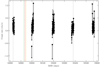 |
Fig. 1. eROSITA light curve of eRASSU J052914.9−662446 in the five epochs from eRASS0 to the beginning of eRASS5. Each point represents a single scan over the source. The dotted green, red, and orange lines indicate the date of the SALT, Swift, and NuSTAR follow-up observations, respectively. The dotted black lines indicate the formal transitions between different eRASSs. Error bars in the y-direction show the 1σ uncertainties assuming Poisson statistics. Count rates of bins with fewer than ten counts are plotted as 1σ upper limits. |
We investigated variability within single survey epochs similar to Stiele et al. (2008) and Sturm et al. (2013), defining the variability Var and significance of the difference S as
where Fmax and σmax define the source flux (background subtracted) and 1σ confidence interval of the time bin for which F − σ is maximum, and analogously, Fmin and σmin of the time bin for which F + σ is minimum. To obtain better statistical treatment, we rebinned the eROSITA light curves of eRASSU J052914.9−662446 by summing original bins until there were at least ten photon counts per time bin. The resulting light curves are displayed as black points in Fig. 2. Using these newly defined bins, we find the strongest variability of Var = 15.0 in epoch 1 with a significance of S = 3.2. Values for Var and S for all epochs can be found in Table 1.
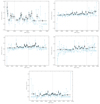 |
Fig. 2. eROSITA light curves of eRASSU J052914.9−662446, where the blue points represent a single scan and the black points are rebinned to a minimum number of ten counts per bin for better statistical treatment. Error bars in the x-direction indicate time bins, and error bars in the y-direction show 1σ uncertainties assuming Poisson statistic. Count rates of bins with fewer thanten counts are plotted as 1σ upper limits. The dotted black lines indicate the formal transitions between different eRASSs. In light blue, we show the original observation pattern obtained by eROSITA. Light curves for epochs 1 (top left), 2 (top right), 3 (centre left), 4 (centre right), and 5 (bottom) are shown, as defined in Table 1. |
Using the data from the dedicated NuSTAR observation, we searched for a periodic signal using a Lomb-Scargle (LS) periodogram analysis (Lomb 1976; Scargle 1982) in the range of 1–5000 s, which covers typical periods seen from HMXB pulsars (Caballero & Wilms 2012). A very strong signal is detected at ∼1412 s (see Fig. 3), indicating the spin period of the neutron star. To determine the spin periods more precisely, an epoch-folding technique was used (Leahy 1987). The best-determined spin period and the uncertainty are given by 1411.8±1.7 s. An additional peak is visible at ∼7000 s. It corresponds to approximately five times the fundamental frequency. However, it is to be noted that red noise is commonly observed in accreting sources and can often appear to be periodic (e.g., Scargle 1981). Therefore, the false-alarm probability of the peaks in the periodogram at lower frequencies can be underestimated (Liu 2008). To estimate the uncertainty on the spin period, we applied a block-bootstrapping method, similarly to Gotthelf et al. (1999) and Carpano et al. (2022), by generating a set of 10 000 light curves. The background-subtracted NuSTAR light curve obtained by combining the two modules and folded with the best-obtained period is shown in Fig. 4. The pulsed fraction, computed by integrating over the 3–78 keV energy band and defined as the ratio of (Imax − Imin)/(Imax + Imin), is 31±3%. We further investigated a possible dependence of the pulse profile on energy by extracting light curves in energy bands with comparable statistical quality. Figure 5 shows that the pulse shape changes from a dip like feature around phase bin ∼0.7 to a broad shoulder-like structure between the energy range of 3–5 keV to 5–10 keV. The pulsed fraction in the energy range of 3–5 keV, 5–10 keV, 10–20 keV, and 20–78 keV is 44±8%, 34±6%, 47±8%, and 28±14%, respectively. Pulsations are not significantly detected above > 20 keV, which is reflected in the low pulsed fraction of the source, in the large fractional errors, and in a lower signal-to-noise ratio in the highest energy band.
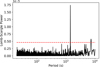 |
Fig. 3. Lomb-Scargle periodogram of eRASSU J052914.9−662446 obtained from the combined NuSTAR data (3.0–30.0 keV). Pulsations are clearly detected with of period of 1412 s. The dashed red line marks the 99.73% confidence level obtained by block-bootstrapping method. |
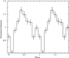 |
Fig. 4. Background-subtracted NuSTAR light curve folded with 1411.8 s showing the pulse profile of eRASSU J052914.9−662446 in the energy band of 3–78 keV. The pulse profile is normalised to the mean count rate of 0.14 cts s−1. |
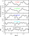 |
Fig. 5. Background-subtracted NuSTAR light curve folded with 1411.8 s showing the pulse profile of eRASSU J052914.9−662446 in the energy ranges and the hardness ratio defined in the figure. The pulse profiles are normalised to the mean count rate of 0.032 cts s−1, 0.064 cts s−1, 0.028 cts s−1, and 0.020 cts s−1. |
3.3. Long-term X-ray variability
Figure 6 shows the long-term X-ray light curve of eRASSU J052914.9−662446 in the energy range of 0.2–2 keV. The fluxes are derived from the XMM-Newton slew, ROSAT PSPC, and HRI observations using the High-Energy Lightcurve Generator (ULS4; Saxton et al. 2022; König et al. 2022) and are derived assuming the spectral parameters from the simultaneous fitting of the eROSITA spectra as given in Table 1. The source was detected twice around MJD 50047 in two ROSAT HRI observations with a flux lower by factor of < 10 than during the eRASS scans. The limit, however, is quite uncertain due to the complex nature of the spectrum at low energies (see Sect. 3.4) and foreground absorption.
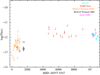 |
Fig. 6. Long-term X-ray light curve of eRASSU J052914.9−662446 in the energy range of 0.2–2 keV. Circles and ellipses represent the measured flux in units of erg cm−2 s−1, and the upper limits are shown as arrows. ROSAT PSPC, ROSAT HRI, XMM-Newton (slew), eROSITA, and Swift fluxes are shown in orange, black, blue, and cyan, and magenta, respectively. Flux values except for eROSITA measurements are derived using the High-Energy Lightcurve Generator. |
3.4. Simultaneous spectral fitting of the eROSITA spectra
The spectra of eRASSU J052914.9−662446 extracted from each of the epochs were simultaneously fit to constrain the average spectral model as well as to investigate possible variability between each eRASSn. All spectra were binned to achieve a minimum of one count per spectral bin, and C-statistics was used because of the low statistics. Spectral analysis was performed using XSPEC v12.11.1k (Arnaud 1996). To account for the photoelectric absorption by the Galactic interstellar gas, we used tbabs in XSPEC with interstellar medium abundances following Wilms et al. (2000) with atomic cross sections from Verner et al. (1996). The Galactic column density of 6 × 1020 cm−2 was taken from Dickey & Lockman (1990) and fixed in the fits. For the absorption along the line of sight (which includes the component through the LMC as well as local to the source), when required, we included a second absorption component with elemental abundances fixed at 0.49 solar (Rolleston et al. 2002; Luck et al. 1998). We left the column density for this component free in the fit. Errors were estimated at 90% confidence intervals. A simple absorbed power-law model provided an adequate description of the spectrum. The X-ray spectrum of eRASSU J052914.9−662446 was modelled using a simultaneous fit of the data from epochs 1, 2, 3, 4, and 5 with only the power-law normalisations left free (it was not possible to investigate possible changes in the power-law index in the current work). The potential additional absorption component from within the LMC could not be constrained and did not improve the fit statistics, therefore we only included the Galactic absorption in our final fit. The parameters of the best-fit model are listed in Table 3, and the spectra and best-fit model are plotted in Fig. 7.
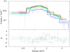 |
Fig. 7. Simultaneous spectral fit of eRASSU J052914.9−662446 using eROSITA spectra of the different epochs defined in Table 1, namely epoch 1 (black), epoch 2 (red), epoch 3 (green), epoch 4 (blue), and epoch 5 (turquoise), together with the best-fit model as histograms. The spectrum for each eRASS is extracted by combining data from the TMs with the on-chip filter. The residuals are plotted in the lower panels. |
Best-fit parameters of eRASSU J052914.9−662446 obtained from the simultaneous fitting of epochs 1–5 spectra (top), epoch 1, and the NuSTAR spectrum (bottom).
3.5. Broadband spectrum of eRASSU J052914.9−662446
The Swift-XRT and the NuSTAR follow-up observations of eRASSU J052914.9−662446 (which were very close in time to epoch 1 of eROSITA) indicated similar flux levels and no significant variation in the X-ray spectrum. Motivated by this, we fitted the eROSITA spectrum from epoch 1 simultaneously with the data from the two NuSTAR modules to constrain the broadband spectral model of eRASSU J052914.9−662446. Constant factors were introduced for each instrument to account for possible absolute cross-calibration differences and time variability and were normalised relative to FPMA. At first, we tried to apply the best-fit model obtained from the simultaneous fitting of the eRASS spectra (Table 3) to the broadband spectrum of the source. Significant residuals were seen both at the low- and high-energy ranges, indicating that the broadband spectrum cannot be described by the same model. The spectra of HMXBs at first approximation can be described by an absorbed power law with an exponential roll-over at high energies. Several empirical functional shapes have been used to describe the broadband spectrum of HMXBs (cutoffpl, fdcut, NPEX, etc.). In most of the sources, the roll-over energy is found to be in the range of 10–50 keV. We found an absorbed cutoffpl model to provide a good description of the broadband spectrum of eRASSU J052914.9−662446. Additional residuals were evident at low energies, and the fit improved significantly by the addition of a partial covering absorber model, which is also often required to model the low-energy part of the X-ray spectrum of HMXBs (see, e.g., Maitra et al. 2012). The difference corresponded to Δcstat = 15 for two degrees of freedom. In contrast, the addition of a blackbody component did not further improve the fit. The best-fit model is summarised in Table 3, and the best-fit spectrum is displayed in Fig. 8.
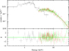 |
Fig. 8. Simultaneous fit of eRASSU J052914.9−662446 using the eRASS1 (black) and the NuSTAR data from the two modules FPMA (red) and FPMB (green). The upper panel shows the best-fit spectrum along with the best-fit model (solid black line), and the bottom panel shows the residuals from the fit. The spectrum has been rebinned only for visual clarity. |
3.6. OGLE monitoring of the optical counterpart
OGLE observed the optical counterpart of eRASSU J052914.9−662446 for 10 years. The I- and V-band light curves are shown in Fig. 9, together with the temporal evolution of the V − I colour index. The light curves show short-term variations on timescales of ∼150 days with amplitudes of ∼0.2 mag in I, superimposed on a slower brightness change over the full observation period. At the beginning of the monitoring, the system was brighter in V than in I, but during the initial brightness decay, it faded faster in V, which resulted in an increase in the V − I colour index to zero about 1000 days after the beginning of the monitoring. After this, the I-band brightness started to rise again, but the reddening continued, although at a lower rate (Fig. 9 bottom panel and Fig. 10).
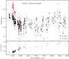 |
Fig. 9. Long term optical variability of eRASSU J052914.9−662446 Top: OGLE-IV light curves in the I (black) and V band (red). Bottom:V − I colour index using I-band data interpolated to the times of the V-band measurements. |
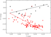 |
Fig. 10. V − I colour index as derived for Fig. 9 as a function of I-band magnitude. Data taken before and after HJD 2456500 are marked in red and black, respectively. The arrows indicate the temporal evolution. |
The OGLE I-band light curve shows short-term variability by about 0.2 mag on timescales between 100 and 200 days. We searched for periodic variations between 20 days and 500 days, which is the typical range of orbital periods found for BeXRBs (Haberl & Sturm 2016). The LS periodogram revealed the strongest peak at a period of ∼151 d (Fig. 11, top), but in addition, many formally significant peaks were observed due to the various variability timescales in the light curve. Therefore, we subtracted a smoothed light curve (derived by applying a Savitzky–Golay filter with a window length of 211 data points; Savitzky & Golay 1964) to remove the long-term trends (see also Haberl et al. 2022b; Maitra et al. 2019). This strongly suppresses the peaks at periods longer than ∼180 days in the LS periodogram (Fig. 11, bottom). However, some peaks between 180 and 300 days remain formally significant, but their broad appearance further indicates an origin from aperiodic variability. All remaining significant peaks around 151 days can be attributed to aliases with the total length of the OGLE monitoring of 3360 days (peaks at 143 and 160 days) or with seasonal effects (a one-year alias at 107 days and an unresolved peak at 135 days caused by three and four years). After the detrending of the light curve, the signal of the ∼151 d period strongly increases in significance and most likely indicates the orbital period of the binary system (see Fig. 12).
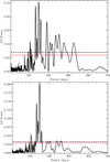 |
Fig. 11. Lomb-Scargle periodograms derived from the measured OGLE I-band light curve (top) and after removing the long-term variation shown in Fig. 9 (bottom). The dashed red and black lines mark the 95% and 99% confidence levels. |
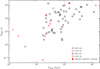 |
Fig. 12. HMXBs in the Magellanic Clouds: Spin period of the neutron star vs orbital period. BeXRBs and (Roche-lobe filling) supergiant systems are found at different locations in this diagram. |
3.7. SALT spectrum
The spectrum obtained by the RSS on SALT is presented in Fig. 13. It is dominated by a double-peaked Hα emission line. The measured line equivalent width (EW) is −8.32 ű0.37 Å with a full width at half maximum (FWHM) of 16.72 ű0.11 Å, which confirms the Be/X-ray binary nature of the source. From the flux-calibrated SALT spectrum, a V-band magnitude of 14.71±0.05 is inferred.
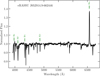 |
Fig. 13. Optical spectrum of eRASSU J052914.9−662446 obtained on 2020 March 20, using the RSS on SALT. The rest wavelengths of the Balmer lines are marked. |
4. Discussion
We report the broadband timing and spectral analysis of the newly discovered source eRASSU J052914.9−662446 through eROSITA, Swift, and NuSTAR data in X-rays and OGLE and SALT RSS data at optical wavelength. We reported the discovery of the spin and the possible orbital period of the system in detail and establish eRASSU J052914.9−662446 as an X-ray binary pulsar. Furthermore, through optical spectroscopic observations and the Hα emission, the source is identified as a Be X-ray binary pulsar in the LMC. The long spin period of the neutron star places eRASSU J052914.9−662446 at the top of the spin period – orbital period diagram assuming the condition of spin equilibrium ((Fig. 12; Corbet 1986); for a more recent version, see, e.g., Mason et al. 2009; Kretschmar et al. 2019). The Corbet diagram also indicates that the LMC BeXRBs seem to lie at the edge of the phase-space occupied by the MC BeXRBs. The results, however, might show observational biases because only a relatively smaller number of systems is known in the LMC compared to the SMC. The source further adds to the recently growing class of highly magnetised, slowly rotating neutron stars (≥1000 s), many of which have been discovered in the Magellanic Clouds (Vasilopoulos et al. 2018; Maitra et al. 2021; Tsygankov et al. 2020, and references therein). It also helps understanding the physics of accretion and the interplay of the accretion torque and magnetic field of the neutron star in these systems, as discussed below.
4.1. Long-term Be-disk/neutron star interaction
The long-term variability in the X-ray regime covers nearly two decades and indicates that although eRASSU J052914.9−662446 was in the field of view of several ROSAT PSPC and HRI pointed observations in the 1990s, it was detected only twice in ∼1995 (MJD 50047) with a flux lower by at least factor of 10 than indicated by the recent eRASS surveys. The V- and I-band variability and the V − I colour index also exhibit an interesting pattern over the past decade. The source was detected initially with a much brighter but rapidly decreasing V-band magnitude that decayed by 0.3 mag on a timescale of ∼500 days. Since a major contributor of the V-band brightness is attributed to the inner circumstellar disk (Yan et al. 2012a,b), the above occurrence can by explained by the cessation of mass supply from the central Be star, causing a depletion in the innermost part of the circumstellar disk and corresponding decay in the V-band brightness. Rivinius et al. (2001), Meilland et al. (2006) and Yan et al. (2016) suggested that the development of a low-density region in the inner circumstellar disk can follow weeks to months after an outburst of the BeXRB. The above behaviour indicates a possible outburst of eRASSU J052914.9−662446 that might have been missed by X-ray monitoring facilities. Following the rapid decline of the V magnitude, the V − I colour index increased to zero and the optical spectrum subsequently reddened, with a gradually growing contribution of the I-band magnitude. This indicates a growing outer part of the circumstellar disk and an increase in the corresponding disk size. The recent detection of eRASSU J052914.9−662446 in an X-ray bright state by eROSITA was unfortunately not covered by OGLE monitoring observations. However, the V-band magnitude of 14.71±0.05, which was obtained from the SALT spectrum, is at the faintest observed level during the OGLE monitoring (14.716±0.003 on HJD 2457719.7, Fig. 9). The relatively strong Hα emission line during this time suggests that the outer disk was dominant and would have resulted in increased reddening, consistent with the scenario described above. In addition, the positive correlation between the I-band magnitude and the colour suggests that the disk is oriented at low to intermediate inclination angles relative to us (see Monageng et al. 2020, and references therein). Using the relation between the FWHM and EW of the Hα line from Hanuschik et al. (1988), the projected rotational velocity of the star, v sin i, can be estimated,
![Mathematical equation: $$ \begin{aligned} \log \left[ \frac{FWHM}{2 ({v} \sin i)} \right] = -0.2\log (-EW) + 0.11 .\end{aligned} $$](/articles/aa/full_html/2023/01/aa44328-22/aa44328-22-eq18.gif) (1)
(1)
We obtain v sin i ≈ 453 km s−1 from our measured parameters. Zorec et al. (2016) showed that the rotational speeds, v, of Be stars have a range in the fraction of the critical velocity of 0.3 < v/vc < 0.95. When we assume an upper limit of the critical velocity of early-type Be stars, v ≈ 600 km s−1 (Porter 1996), this gives a minimum inclination angle of i ≈ 52° that is consistent with the above scenario.
4.2. Complex-absorber scenario and the non-detection of CRSF for eRASSU J052914.9−662446
The broadband X-ray spectrum is typical of HMXBs and can be described empirically with an absorbed power law with a photon index ∼1 and an exponential rollover cutoff at ∼10 keV. The low-energy spectrum (< 2 keV) is quite complex, however, and can be described by a partial covering absorbing column that covers 84% of the source. The presence of a complex absorber is also supported by the X-ray timing properties of the source, as the morphology of the pulse profile (Fig. 4) exhibits a narrow (0.1 in phase) dip at phase ∼0.7. Pulse profiles of Be/X-ray binary pulsars are known to be complex in low (< 10 keV) X-ray energy ranges with multiple emission peaks and sometimes narrow absorption dips. Phase-resolved spectroscopy in some of the Galactic BeXRBs revealed that matter in the accretion streams partially obscures the emitted radiation causing the dips (e.g., Maitra et al. 2012; Naik et al. 2013). Examples in the Magellanic Clouds are Swift J053041.9−665426 = LXP 28.8 (Vasilopoulos et al. 2013), XMMU J005929.0−723703 = SXP 202b (Haberl et al. 2008), and XMMU J045736.9−692727 (Haberl et al. 2022b).
The magnetic field strength of the neutron star can be robustly determined from an observed cyclotron resonance scattering feature (CRSF) centroid energy as Ecyc (determined from Obs. 1), and is given as
 (2)
(2)
where B12 is the field strength in units of 1012 G; z ∼ 0.3 is the gravitational redshift in the scattering region for standard neutron star parameters. CRSFs are often observed as broad, shallow features that can be difficult to detect against the continuum spectrum. Although we did not find any evidence for a statistically significant feature in the X-ray spectrum, we computed an upper limit on the depth of a putative CRSF by varying the line centroid energy in the range of 7–25 keV (the energy range in which the signal-to-noise ratio is highest) in steps of 500 eV and by fixing the width at 20% its centroid energy (see, e.g., Maitra 2017; Staubert et al. 2019, for typically observed ratios of energy to width). We obtained a highest line depth of τc ∼ 0.8 at an energy of 17 keV. The CRSF energy would imply a magnetic field strength of B ≈ 1012 G for the NS.
4.3. Subsonic accretion onto a slowly rotating highly magnetised neutron star in eRASSU J052914.9−662446
A plausible explanation for low X-ray luminosity (∼1035–1036 erg s−1) and slowly rotating (∼1000 s) neutron stars is that these systems may be quasi-spherically accreting from stellar winds. In this regime, subsonic or settling accretion occurs when the plasma remains hot until it meets the magnetospheric boundary. A hot quasi-spherical shell is formed around the magnetosphere as the Compton cooling timescale of plasma above the magnetosphere is much shorter than the timescale of the freely falling fresh matter that is gravitationally captured from the stellar wind (Shakura et al. 2012). The actual accretion rate onto the neutron star is determined by the ability of the plasma to enter the magnetosphere due to the Rayleigh-Taylor instability and varies between 0.1–0.5 of the Bondi mass accretion rate (Shakura et al. 2012, 2018; Shakura & Postnov 2017). The shell mediates the angular momentum transport to or from the rotating neutron star, and both spin-up and spin-down is possible depending on the sign of the angular momentum difference between the matter being accreted and the magnetospheric boundary. Under the assumption of spin equilibrium, the spin period can be derived as in Shakura & Postnov (2017). Ignoring the dimensionless theory parameters Π0, ζ of about unity, we find
![Mathematical equation: $$ \begin{aligned} P_\mathrm{eq} \approx 1000[\mathrm{s} ]\ \mu _{30}^{12/11} \left(\frac{P_\mathrm{b} }{10\,\mathrm{d}}\right)\dot{M}_{16}^{-4/11}{v}_8^4\,. \end{aligned} $$](/articles/aa/full_html/2023/01/aa44328-22/aa44328-22-eq20.gif) (3)
(3)
Here the parameters are normalised to the typical values; μ30 ≡ μ/(1030 G cm3), Pb is the binary orbital period (the orbit is assumed to be circular), Ṁ16 ≡ Ṁ/(1016 g s−1) is the accretion rate onto the neutron star surface corresponding to an X-ray luminosity of Lx = 0.15 Ṁc2, and v8 ≡ v/(1000 km s−1) is the stellar wind velocity relative to the neutron star. Substituting P ≈ 1412 s, Ṁ16 ≃ 7, and Pb = 151 d, we find
 (4)
(4)
We note that the estimate of the magnetic field of the neutron star is strongly dependent on the stellar wind velocity. For a value of 1000 km s−1, B ≈ 1012 G, which indicates the typical magnetic field strength of an NS.
It should be noted that the main source of uncertainty in the estimation of B using the quasi-spherical accreting scenario is the wind velocity. The stellar wind of a Be star is highly anisotropic in nature. At its poles, the wind velocities are high but the density is low, while it is denser near the equator but much slower due to the presence of the disk (Poeckert & Marlborough 1978; Lamers & Pauldrach 1991). Waters & van Kerkwijk (1989) provided a prescription for estimating the typical wind velocity of BeXRBs as described below. From the measured Hα equivalent width (Sect. 3.7) of −8.32 Å ± 0.37 Å, the size of the Be disk can be estimated using the relation from Grundstrom & Gies (2006) and Grundstrom et al. (2007) to be R ∼ 4 Rs, where Rs is the radius of the star. Furthermore, following Eqs. (4) and (5) of Waters & van Kerkwijk (1989), the upper limit on the radial velocity vr component and the rotational wind vw component can be derived as 120 km s−1 and 74 km s−1, respectively, assuming maximum values for v0 = 30 km s−1, n = 3.2, and veq = 300 km s−1 (see Keller 2004, for the range of the rotational velocity of Be stars observed in the LMC). This leads to a value of vrw ≈ 150 km s−1 for the net wind velocity component. To compute the wind velocity relative to the NS, the orbital motion needs to be taken into account. Assuming Pb = 151 days and a Be star with mass ≈10 M⊙, we obtain a velocity that is also ≈100 km s−1 assuming a circular orbit with zero eccentricity. This leads to an upper limit of ≈250 km s−1 for the relative velocity. However, a majority of the observed BeXRBs have eccentric orbits. In order to account for the possible eccentricity of the orbit in eRASSU J052914.9−662446, we looked at the sample of BeXRBs in the SMC with reliably measured eccentricity values (Townsend et al. 2011). A highly eccentric orbit from the maximum measured value of e = 0.8 leads to a maximum velocity of ≈300 km s−1 at perigee and an upper limit of the relative velocity of ≈450 km s−1. These values lead to a lower limit of the magnetic field strength between 4 × 10¹³ − 1014 G for the subsonic accretion scenario, indicating a highly magnetised NS or a magnetar.
It is also worth mentioning that the magnetic field strength assuming disk accretion and using the standard prescription of Ghosh & Lamb (1979) under the equilibrium hypothesis leads to an estimation of a factor of ∼10 or higher B for these slowly rotating pulsars. Furthermore, future monitoring programs are essential to determine the validity of the assumption of spin equilibrium of the system, and to decide whether the pulsar is spinning up or down.
5. Conclusions
The main results are summarised as below:
We reported the discovery of pulsations at a period of 1412 s from the newly discovered source eRASSU J052914.9−662446 in the LMC. Pulsations are detected in a broad energy range of 0.2–20 keV, and the pulse profile does not show a strong dependence on energy.
The X-ray position is consistent with a star with magnitudes and colours indicative of an early spectral type. Furthermore, our optical spectroscopic observations revealed the existence of Hα emission, and the source is identified as a Be X-ray binary pulsar in the LMC.
The broadband X-ray spectrum is typical of HMXBs and can be described empirically with an absorbed power law with a photon index ∼1 and an exponential rollover cutoff at ∼10 keV. No evidence of a CRSF was found in the broadband X-ray spectrum. We obtained an upper limit of τc ∼ 0.8 on the depth of a CRSF at a centroid energy of 17 keV for a typical magnetic field strength of ≈1012 G for an NS. The estimation of B under the assumption of spin equilibrium for a quasi-spherical subsonic accretion scenario for eRASSU J052914.9−662446 indicates a much higher B value of 4 × 10¹³ − 1014 G for the NS, but is prone to several uncertainties, especially in the estimation of the wind velocity.
Decadal monitoring with OGLE revealed a variable optical counterpart with a periodicity of ∼151 days in the I band, which indicates the orbital period of the system. At the beginning of the optical monitoring, the system was brighter in V, which decayed very rapidly, resulting in an increase to zero of the V − I colour index, and after the I-band brightness started rising again, the reddening of the system continued. eRASSU J052914.9−662446 was serendipitously located in the field of view of several ROSAT PSPC and HRI pointed observations and was detected only twice in ∼1995 (MJD 50047) with a flux lower by at least factor of 10 than indicated by the recent eRASS surveys. This suggests a variable nature in the X-ray regime.
Future monitoring of eRASSU J052914.9−662446 in the X-ray regime will provide insights on the spin evolution of the system, validate the assumption of spin equilibrium, and ultimately provide robust estimates on the magnetic field strength of the neutron star.
Acknowledgments
We thank the referee for useful comments and suggestions. This work is based on data from eROSITA, the soft X-ray instrument aboard SRG, a joint Russian-German science mission supported by the Russian Space Agency (Roskosmos), in the interests of the Russian Academy of Sciences represented by its Space Research Institute (IKI), and the Deutsches Zentrum für Luft- und Raumfahrt (DLR). The SRG spacecraft was built by Lavochkin Association (NPOL) and its subcontractors, and is operated by NPOL with support from the Max Planck Institute for Extraterrestrial Physics (MPE). The development and construction of the eROSITA X-ray instrument was led by MPE, with contributions from the Dr. Karl Remeis-Observatory Bamberg & ECAP (FAU Erlangen-Nürnberg), the University of Hamburg Observatory, the Leibniz Institute for Astrophysics Potsdam (AIP), and the Institute for Astronomy and Astrophysics of the University of Tübingen, with the support of DLR and the Max Planck Society. The Argelander Institute for Astronomy of the University of Bonn and the Ludwig Maximilians Universität Munich also participated in the science preparation for eROSITA. The eROSITA data shown here were processed using the eSASS software system developed by the German eROSITA consortium. This work used observations obtained with XMM-Newton, an ESA science mission with instruments and contributions directly funded by ESA Member States and NASA. The XMM-Newton project is supported by the DLR and the Max Planck Society. This work is partially supported by the Bundesministerium für Wirtschaft und Energie through the Deutsches Zentrum für Luft- und Raumfahrt e.V. (DLR) under the grant number FKZ 50 QR 2102. This research has made use of the VizieR catalogue access tool, CDS, Strasbourg, France. The original description of the VizieR service was published in A&A, 143, 23.
References
- Antoniou, V., & Zezas, A. 2016, MNRAS, 459, 528 [Google Scholar]
- Arnaud, K. A. 1996, in Astronomical Data Analysis Software and Systems V, eds. G. H. Jacoby, & J. Barnes, ASP Conf. Ser., 101, 17 [NASA ADS] [Google Scholar]
- Babusiaux, C., Fabricius, C., Khanna, S., et al. 2022, A&A, in press, https://doi.org/10.1051/0004-6361/202243790 [Google Scholar]
- Brunner, H., Liu, T., Lamer, G., et al. 2022, A&A, 661, A1 [NASA ADS] [CrossRef] [EDP Sciences] [Google Scholar]
- Buckley, D. A. H., Swart, G. P., & Meiring, J. G. 2006, in Society of Photo-Optical Instrumentation Engineers (SPIE) Conference Series, ed. L. M. Stepp, SPIE Conf. Ser., 6267, 62670Z [NASA ADS] [Google Scholar]
- Burrows, D. N., Hill, J. E., Nousek, J. A., et al. 2005, Space Sci. Rev., 120, 165 [Google Scholar]
- Caballero, I., & Wilms, J. 2012, Mem. Soc. Astron. Ital., 83, 230 [Google Scholar]
- Carpano, S., Haberl, F., Maitra, C., et al. 2022, A&A, 661, A20 [NASA ADS] [CrossRef] [EDP Sciences] [Google Scholar]
- Cash, W. 1979, ApJ, 228, 939 [Google Scholar]
- Corbet, R. H. D. 1986, MNRAS, 220, 1047 [NASA ADS] [CrossRef] [Google Scholar]
- Crawford, S. M., Still, M., Schellart, P., et al. 2010, in Observatory Operations: Strategies, Processes, and Systems III, eds. D. R. Silva, A. B. Peck, & B. T. Soifer, SPIE Conf. Ser., 7737, 773725 [NASA ADS] [CrossRef] [Google Scholar]
- Cutri, R. M., Skrutskie, M. F., van Dyk, S., et al. 2003, VizieR Online Data Catalog, 2246 [Google Scholar]
- Dickey, J. M., & Lockman, F. J. 1990, ARA&A, 28, 215 [Google Scholar]
- Evans, P. A., Beardmore, A. P., Page, K. L., et al. 2007, A&A, 469, 379 [NASA ADS] [CrossRef] [EDP Sciences] [Google Scholar]
- For, B. Q., Staveley-Smith, L., Hurley-Walker, N., et al. 2018, MNRAS, 480, 2743 [NASA ADS] [CrossRef] [Google Scholar]
- Gehrels, N., Chincarini, G., Giommi, P., et al. 2004, ApJ, 611, 1005 [Google Scholar]
- Ghosh, P., & Lamb, F. K. 1979, ApJ, 234, 296 [Google Scholar]
- Gotthelf, E. V., Vasisht, G., & Dotani, T. 1999, ApJ, 522, L49 [NASA ADS] [CrossRef] [Google Scholar]
- Grundstrom, E. D., & Gies, D. R. 2006, ApJ, 651, L53 [NASA ADS] [CrossRef] [Google Scholar]
- Grundstrom, E. D., Caballero-Nieves, S. M., Gies, D. R., et al. 2007, ApJ, 656, 437 [NASA ADS] [CrossRef] [Google Scholar]
- Haberl, F., & Sturm, R. 2016, A&A, 586, A81 [NASA ADS] [CrossRef] [EDP Sciences] [Google Scholar]
- Haberl, F., Eger, P., & Pietsch, W. 2008, A&A, 489, 327 [NASA ADS] [CrossRef] [EDP Sciences] [Google Scholar]
- Haberl, F., Maitra, C., Carpano, S., et al. 2020, ATel, 13609, 1 [Google Scholar]
- Haberl, F., Salganik, A., Maitra, C., et al. 2021, ATel, 15133, 1 [NASA ADS] [Google Scholar]
- Haberl, F., Maitra, C., Carpano, S., et al. 2022a, A&A, 661, A25 [NASA ADS] [CrossRef] [EDP Sciences] [Google Scholar]
- Haberl, F., Maitra, C., Vasilopoulos, G., et al. 2022b, A&A, 662, A22 [NASA ADS] [CrossRef] [EDP Sciences] [Google Scholar]
- Harrison, F. A., Craig, W. W., Christensen, F. E., et al. 2013, ApJ, 770, 103 [Google Scholar]
- Keller, S. C. 2004, PASA, 21, 310 [NASA ADS] [CrossRef] [Google Scholar]
- König, O., Saxton, R. D., Kretschmar, P., et al. 2022, Astron. Comput., 38, 100529 [CrossRef] [Google Scholar]
- Kretschmar, P., Fürst, F., Sidoli, L., et al. 2019, New A Rev., 86, 101546 [NASA ADS] [CrossRef] [Google Scholar]
- Lamers, H. J. G., & Pauldrach, A. W. A. 1991, A&A, 244, L5 [NASA ADS] [Google Scholar]
- Leahy, D. A. 1987, A&A, 180, 275 [NASA ADS] [Google Scholar]
- Liu, J.-F. 2008, ApJS, 177, 181 [NASA ADS] [CrossRef] [Google Scholar]
- Lomb, N. R. 1976, Ap&SS, 39, 447 [Google Scholar]
- Luck, R. E., Moffett, T. J., Barnes, T. G., & Gieren, W. P., 1998, AJ, 115, 605 [NASA ADS] [CrossRef] [Google Scholar]
- Maitra, C. 2017, J. Astrophys. Astron., 38, 50 [NASA ADS] [CrossRef] [Google Scholar]
- Maitra, C., Paul, B., & Naik, S. 2012, MNRAS, 420, 2307 [NASA ADS] [CrossRef] [Google Scholar]
- Maitra, C., Haberl, F., Filipović, M. D., et al. 2019, MNRAS, 490, 5494 [Google Scholar]
- Maitra, C., Haberl, F., Carpano, S., et al. 2020a, ATel, 13610, 1 [Google Scholar]
- Maitra, C., Haberl, F., Koenig, O., et al. 2020b, ATel, 13650, 1 [NASA ADS] [Google Scholar]
- Maitra, C., Haberl, F., Vasilopoulos, G., et al. 2021, A&A, 647, A8 [NASA ADS] [CrossRef] [EDP Sciences] [Google Scholar]
- Mason, A. B., Clark, J. S., Norton, A. J., Negueruela, I., & Roche, P. 2009, A&A, 505, 281 [NASA ADS] [CrossRef] [EDP Sciences] [Google Scholar]
- Meilland, A., Stee, P., Zorec, J., & Kanaan, S. 2006, A&A, 455, 953 [NASA ADS] [CrossRef] [EDP Sciences] [Google Scholar]
- Monageng, I. M., Coe, M. J., Buckley, D. A. H., et al. 2020, MNRAS, 496, 3615 [NASA ADS] [CrossRef] [Google Scholar]
- Naik, S., Maitra, C., Jaisawal, G. K., & Paul, B. 2013, ApJ, 764, 158 [NASA ADS] [CrossRef] [Google Scholar]
- Pietrzyński, G., Graczyk, D., Gieren, W., et al. 2013, Nature, 495, 76 [Google Scholar]
- Pietrzyński, G., Graczyk, D., Gallenne, A., et al. 2019, Nature, 567, 200 [Google Scholar]
- Poeckert, R., & Marlborough, J. M. 1978, ApJS, 38, 229 [CrossRef] [Google Scholar]
- Porter, J. M. 1996, MNRAS, 280, L31 [NASA ADS] [CrossRef] [Google Scholar]
- Predehl, P., Andritschke, R., Arefiev, V., et al. 2021, A&A, 647, A1 [EDP Sciences] [Google Scholar]
- Riess, A. G., Casertano, S., Yuan, W., Macri, L. M., & Scolnic, D. 2019, ApJ, 876, 85 [Google Scholar]
- Rivinius, T., Baade, D., Štefl, S., & Maintz, M. 2001, A&A, 379, 257 [NASA ADS] [CrossRef] [EDP Sciences] [Google Scholar]
- Rolleston, W. R. J., Trundle, C., & Dufton, P. L. 2002, A&A, 396, 53 [NASA ADS] [CrossRef] [EDP Sciences] [Google Scholar]
- Savitzky, A., & Golay, M. J. E. 1964, Anal. Chem., 36, 1627 [Google Scholar]
- Saxton, R. D., König, O., Descalzo, M., et al. 2022, Astron. Comput., 38, 100531 [NASA ADS] [CrossRef] [Google Scholar]
- Scargle, J. D. 1981, ApJS, 45, 1 [NASA ADS] [CrossRef] [Google Scholar]
- Scargle, J. D. 1982, ApJ, 263, 835 [Google Scholar]
- Shakura, N., & Postnov, K. 2017, Proceedings of Sciences, 288 (APCS2016), 040 [Google Scholar]
- Shakura, N., Postnov, K., Kochetkova, A., & Hjalmarsdotter, L. 2012, MNRAS, 420, 216 [Google Scholar]
- Shakura, N., Postnov, K., Kochetkova, A., & Hjalmarsdotter, L. 2018, in Astrophysics and Space Science Library, 454, 331 [NASA ADS] [CrossRef] [Google Scholar]
- Staubert, R., Trümper, J., Kendziorra, E., et al. 2019, A&A, 622, A61 [NASA ADS] [CrossRef] [EDP Sciences] [Google Scholar]
- Stiele, H., Pietsch, W., Haberl, F., & Freyberg, M. 2008, A&A, 480, 599 [NASA ADS] [CrossRef] [EDP Sciences] [Google Scholar]
- Sturm, R., Haberl, F., Pietsch, W., et al. 2013, A&A, 558, A3 [NASA ADS] [CrossRef] [EDP Sciences] [Google Scholar]
- Townsend, L. J., Coe, M. J., Corbet, R. H. D., & Hill, A. B. 2011, MNRAS, 416, 1556 [NASA ADS] [CrossRef] [Google Scholar]
- Tsygankov, S. S., Doroshenko, V., Mushtukov, A. A., et al. 2020, A&A, 637, A33 [NASA ADS] [CrossRef] [EDP Sciences] [Google Scholar]
- Udalski, A., Szymanski, M., Kaluzny, J., Kubiak, M., & Mateo, M. 1992, Acta Astron., 42, 253 [NASA ADS] [Google Scholar]
- Udalski, A., Szymanski, M. K., Soszynski, I., & Poleski, R. 2008, Acta Astron., 58, 69 [NASA ADS] [Google Scholar]
- Udalski, A., Szymański, M. K., & Szymański, G. 2015, Acta Astron., 65, 1 [NASA ADS] [Google Scholar]
- Vasilopoulos, G., Maggi, P., Haberl, F., et al. 2013, A&A, 558, A74 [NASA ADS] [CrossRef] [EDP Sciences] [Google Scholar]
- Vasilopoulos, G., Maitra, C., Haberl, F., Hatzidimitriou, D., & Petropoulou, M. 2018, MNRAS, 475, 220 [Google Scholar]
- Verner, D. A., Ferland, G. J., Korista, K. T., & Yakovlev, D. G. 1996, ApJ, 465, 487 [Google Scholar]
- Waters, L. B. F. M., & van Kerkwijk, M. H. 1989, A&A, 223, 196 [Google Scholar]
- Wilms, J., Allen, A., & McCray, R. 2000, ApJ, 542, 914 [Google Scholar]
- Yan, J., Li, H., & Liu, Q. 2012a, ApJ, 744, 37 [NASA ADS] [CrossRef] [Google Scholar]
- Yan, J., Zurita Heras, J. A., Chaty, S., Li, H., & Liu, Q. 2012b, ApJ, 753, 73 [NASA ADS] [CrossRef] [Google Scholar]
- Yan, J., Zhang, P., Liu, W., & Liu, Q. 2016, AJ, 151, 104 [NASA ADS] [CrossRef] [Google Scholar]
- Zaritsky, D., Harris, J., Thompson, I. B., & Grebel, E. K. 2004, AJ, 128, 1606 [Google Scholar]
- Zorec, J., Frémat, Y., Domiciano de Souza, A., et al. 2016, A&A, 595, A132 [NASA ADS] [CrossRef] [EDP Sciences] [Google Scholar]
All Tables
Best-fit parameters of eRASSU J052914.9−662446 obtained from the simultaneous fitting of epochs 1–5 spectra (top), epoch 1, and the NuSTAR spectrum (bottom).
All Figures
|
Fig. 1. eROSITA light curve of eRASSU J052914.9−662446 in the five epochs from eRASS0 to the beginning of eRASS5. Each point represents a single scan over the source. The dotted green, red, and orange lines indicate the date of the SALT, Swift, and NuSTAR follow-up observations, respectively. The dotted black lines indicate the formal transitions between different eRASSs. Error bars in the y-direction show the 1σ uncertainties assuming Poisson statistics. Count rates of bins with fewer than ten counts are plotted as 1σ upper limits. |
| In the text | |
|
Fig. 2. eROSITA light curves of eRASSU J052914.9−662446, where the blue points represent a single scan and the black points are rebinned to a minimum number of ten counts per bin for better statistical treatment. Error bars in the x-direction indicate time bins, and error bars in the y-direction show 1σ uncertainties assuming Poisson statistic. Count rates of bins with fewer thanten counts are plotted as 1σ upper limits. The dotted black lines indicate the formal transitions between different eRASSs. In light blue, we show the original observation pattern obtained by eROSITA. Light curves for epochs 1 (top left), 2 (top right), 3 (centre left), 4 (centre right), and 5 (bottom) are shown, as defined in Table 1. |
| In the text | |
|
Fig. 3. Lomb-Scargle periodogram of eRASSU J052914.9−662446 obtained from the combined NuSTAR data (3.0–30.0 keV). Pulsations are clearly detected with of period of 1412 s. The dashed red line marks the 99.73% confidence level obtained by block-bootstrapping method. |
| In the text | |
|
Fig. 4. Background-subtracted NuSTAR light curve folded with 1411.8 s showing the pulse profile of eRASSU J052914.9−662446 in the energy band of 3–78 keV. The pulse profile is normalised to the mean count rate of 0.14 cts s−1. |
| In the text | |
|
Fig. 5. Background-subtracted NuSTAR light curve folded with 1411.8 s showing the pulse profile of eRASSU J052914.9−662446 in the energy ranges and the hardness ratio defined in the figure. The pulse profiles are normalised to the mean count rate of 0.032 cts s−1, 0.064 cts s−1, 0.028 cts s−1, and 0.020 cts s−1. |
| In the text | |
|
Fig. 6. Long-term X-ray light curve of eRASSU J052914.9−662446 in the energy range of 0.2–2 keV. Circles and ellipses represent the measured flux in units of erg cm−2 s−1, and the upper limits are shown as arrows. ROSAT PSPC, ROSAT HRI, XMM-Newton (slew), eROSITA, and Swift fluxes are shown in orange, black, blue, and cyan, and magenta, respectively. Flux values except for eROSITA measurements are derived using the High-Energy Lightcurve Generator. |
| In the text | |
|
Fig. 7. Simultaneous spectral fit of eRASSU J052914.9−662446 using eROSITA spectra of the different epochs defined in Table 1, namely epoch 1 (black), epoch 2 (red), epoch 3 (green), epoch 4 (blue), and epoch 5 (turquoise), together with the best-fit model as histograms. The spectrum for each eRASS is extracted by combining data from the TMs with the on-chip filter. The residuals are plotted in the lower panels. |
| In the text | |
|
Fig. 8. Simultaneous fit of eRASSU J052914.9−662446 using the eRASS1 (black) and the NuSTAR data from the two modules FPMA (red) and FPMB (green). The upper panel shows the best-fit spectrum along with the best-fit model (solid black line), and the bottom panel shows the residuals from the fit. The spectrum has been rebinned only for visual clarity. |
| In the text | |
|
Fig. 9. Long term optical variability of eRASSU J052914.9−662446 Top: OGLE-IV light curves in the I (black) and V band (red). Bottom:V − I colour index using I-band data interpolated to the times of the V-band measurements. |
| In the text | |
|
Fig. 10. V − I colour index as derived for Fig. 9 as a function of I-band magnitude. Data taken before and after HJD 2456500 are marked in red and black, respectively. The arrows indicate the temporal evolution. |
| In the text | |
|
Fig. 11. Lomb-Scargle periodograms derived from the measured OGLE I-band light curve (top) and after removing the long-term variation shown in Fig. 9 (bottom). The dashed red and black lines mark the 95% and 99% confidence levels. |
| In the text | |
|
Fig. 12. HMXBs in the Magellanic Clouds: Spin period of the neutron star vs orbital period. BeXRBs and (Roche-lobe filling) supergiant systems are found at different locations in this diagram. |
| In the text | |
|
Fig. 13. Optical spectrum of eRASSU J052914.9−662446 obtained on 2020 March 20, using the RSS on SALT. The rest wavelengths of the Balmer lines are marked. |
| In the text | |
Current usage metrics show cumulative count of Article Views (full-text article views including HTML views, PDF and ePub downloads, according to the available data) and Abstracts Views on Vision4Press platform.
Data correspond to usage on the plateform after 2015. The current usage metrics is available 48-96 hours after online publication and is updated daily on week days.
Initial download of the metrics may take a while.