| Issue |
A&A
Volume 672, April 2023
|
|
|---|---|---|
| Article Number | A131 | |
| Number of page(s) | 12 | |
| Section | Extragalactic astronomy | |
| DOI | https://doi.org/10.1051/0004-6361/202244209 | |
| Published online | 12 April 2023 | |
Detection of chemo-kinematical structures in Leo I
1
Departamento de Astronomía, Universidad de Concepción, Casilla 160-C, Concepción, Chile
e-mail: This email address is being protected from spambots. You need JavaScript enabled to view it.
2
Observatories of the Carnegie Institution of Washington, 813 Santa Barbara St., Pasadena, CA 91101, USA
3
Centro de Estudios de Física del Cosmos de Aragón (CEFCA), Unidad Asociada al CSIC, Plaza San Juan 1, 44001 Teruel, Spain
4
Department of Physics and Astronomy, Pomona College, 333 N College Way, Claremont, CA 91711, USA
5
Space Telescope Science Institute, 3700 San Martin Drive, Baltimore, MD 21218, USA
Received:
7
June
2022
Accepted:
13
January
2023
Abstract
Context. A variety of formation models for dwarf spheroidal (dSph) galaxies have been proposed in the literature, but generally they have not been quantitatively compared with observations.
Aims. We search for chemodynamical patterns in our observational data set and compare the results with mock galaxies consisting of pure random motions, and simulated dwarfs formed via the dissolving star cluster and tidal stirring models.
Methods. We made use of a new spectroscopic data set for the Milky Way dSph Leo I, combining 288 stars observed with Magellan/IMACS and existing Keck/DEIMOS data, to provide velocity and metallicity measurements for 953 Leo I member stars. We used a specially developed algorithm called BEACON to detect chemo-kinematical patterns in the observed and simulated data.
Results. After analysing the Leo I data, we report the detection of 14 candidate streams of stars that may have originated in disrupted star clusters. The angular momentum vectors of these streams are randomly oriented, consistent with the lack of rotation in Leo I. These results are consistent with the predictions of the dissolving cluster model. In contrast, we find fewer candidate stream signals in mock data sets that lack coherent motions ∼99% of the time. The chemodynamical analysis of the tidal stirring simulation produces streams that share a common orientation of their angular momenta, which is inconsistent with the Leo I data.
Conclusions. Even though it is very difficult to distinguish which of the detected streams are real and which are only noise, we can be certain that there are more streams detected in the observational data of Leo I than expected in pure random data.
Key words: methods: numerical / galaxies: dwarf / galaxies: individual: Leo I / galaxies: kinematics and dynamics / galaxies: formation
© The Authors 2023
 Open Access article, published by EDP Sciences, under the terms of the Creative Commons Attribution License (https://creativecommons.org/licenses/by/4.0), which permits unrestricted use, distribution, and reproduction in any medium, provided the original work is properly cited.
This article is published in open access under the Subscribe to Open model. This email address is being protected from spambots. You need JavaScript enabled to view it. to support open access publication.
1. Introduction
The Local Group consists of about 80 galaxies discovered to date (McConnachie 2012), and this number is expected to grow with observations of future telescopes and surveys. Most of them are dwarf galaxies, orbiting the two larger galaxies, the Milky Way (MW) and Andromeda (M 31). Their classifications range from dwarf irregulars, dwarf ellipticals, and compact ellipticals to dwarf spheroidal (dSph) galaxies, the last composing the majority of the known dwarfs.
Based on their high velocity dispersions and low luminosities, dSph galaxies have high mass-to-light ratios and are believed to be the most dark matter (DM) dominated stellar systems known (Mateo 1998; Walker et al. 2009). They are among the oldest structures and are by far the most numerous galaxies in the Universe; however, due to their intrinsic faintness, the study of dSph galaxies has been very difficult. In the standard hierarchical galaxy formation models, dwarf galaxies are the elemental systems in the Universe; larger galaxies are formed from smaller objects like dwarf galaxies through major and/or minor mergers (Kauffmann et al. 1993; Cole et al. 1994). Thus, it is important to study these galaxies to understand the formation and evolution of normal sized galaxies.
DSph galaxies have a low stellar content and are poor in, or entirely devoid of, gas. The faint and ultra-faint population of dSph galaxies are widely thought to be the smallest DM structures that contain stars (Mateo 1998; Łokas 2009; Walker et al. 2009). The larger classical dSph galaxies are characterized by absolute magnitudes in the range −13 ≤ MV ≤ −9 (Mateo 1998; Belokurov et al. 2007). Their total estimated masses, considering the stars and the DM halo is of the order of 109 M⊙. They exhibit high velocity dispersions (e.g., Simon & Geha 2007; Koch et al. 2009) in the range of 5 − 12 km s−1; the velocity dispersion remains approximately constant with distance from the centre of the galaxy (Kleyna et al. 2002, 2003; Muñoz et al. 2005, 2006; Simon & Geha 2007; Walker et al. 2007).
Leo I is one of the classical dSph galaxies orbiting the MW detected by A. G. Wilson in 1950 (Harrington & Wilson 1950) and described in Hodge (1962), among others. It is one of the most distant MW satellites. At 257 ± 13 kpc (Sohn et al. 2013) and with a half-light radius of 244 ± 2 pc (McConnachie 2012), it is classified as a dSph galaxy (McConnachie 2012), based on its current morphology and lack of gas (Knapp et al. 1978; Grcevich & Putman 2009).
Leo I displays a very extended star formation history (Gallart et al. 1999; Hernandez et al. 2000), and is considered one of the youngest dSph galaxies in our Local Group in terms of average age (Lee et al. 1993; Weisz et al. 2014a,b). Most of the star-forming activity in Leo I happened between 7 Gyr and as recently as 1 Gyr ago (Gallart et al. 1999). Similar to others dwarf galaxies, Leo I has a low metallicity (of the order of [Fe/H] = −1.43 dex; Kirby et al. 2011), contains no globular clusters, and is a purely dispersion-supported system.
Given its distance from the Milky Way and recent star formation history, it provides an important tracer to explore the MW mass (Boylan-Kolchin et al. 2013) and evolution models. Metallicity studies (Bosler et al. 2007), proper motion (Gaia Collaboration 2018; Sohn et al. 2013), and radial velocity measurements (Koch et al. 2009; Sohn et al. 2007) have provided a significant amount of data on the galaxy, which has been extensively analysed by various groups.
Studies using statistical comparisons with simulations and direct comparisons with Jeans spherical dynamical models often yield contradictory pictures. For example, Mateo et al. (2008) found evidence for an extended DM halo by observing a flat velocity dispersion profile at large radii, and Łokas et al. (2008) found a DM profile similar to the stellar profile. Recently, Bustamante-Rosell et al. (2021) measured the central kinematics of Leo I and find that the orbits of the inner stars of the galaxy indicate the presence of a central black hole of 3.3 ± 2 × 10⁶ M⊙. All this, combined with the narrow stellar metallicity displayed by Leo I, its shallow negative metallicity gradient, and its positive age trend (Gullieuszik et al. 2009), make Leo I one of the most exciting dwarf galaxies in the Local Group.
Analysis of the proper motion of Leo I indicate that this galaxy stopped forming stars about 1 Gyr ago, probably due to the pericentric approach to the MW (Sohn et al. 2013; Gaia Collaboration 2018). Previous works have hinted at a turbulent past characterized by alternating periods of intense star formation with quiescent intervals (Gallart et al. 1999; Hernandez et al. 2000).
There are several models that attempt to explain the origin and features of dSph galaxies by considering different mechanisms. Some of them are based on tidal and ram-pressure stripping (Gnedin et al. 1999; Mayer et al. 2007). In these models the dSph galaxies are formed due to the interaction between a rotationally supported dwarf irregular galaxy and a MW-sized host galaxy. These models show that dSph galaxies tend to appear near massive galaxies, but they do not explain the presence of distant isolated dSph galaxies, such as Tucana, Cetus, and Leo T.
The model proposed by D’Onghia et al. (2009) considers a mechanism known as resonant stripping, which can be used to explain the formation of isolated dSph galaxies. Basically, these objects are formed after encounters between dwarf disc galaxies in a process driven by gravitational resonances.
According to the dissolving star cluster scenario (Assmann et al. 2013a,b; Alarcón Jara et al. 2018), a dSph galaxy is formed by the fusion and dissolution of several star clusters (SCs) with low star formation efficiency (SFE), formed within one DM halo. This model does not need gravitational interactions with other galaxies to explain the formation of dSph galaxies, and can therefore can account for the formation of isolated galaxies as well.
Several recent studies have been performed analysing the chemo-kinematical patterns among the stars in multiple dwarf galaxies from the Local Group, applying different methods (Cicuéndez & Battaglia 2018; del Pino et al. 2017; Lora et al. 2019). Using our new extended data set, we are searching for similar chemo-kinematical patterns in the Leo I dSph galaxy.
In the next section we describe the spectroscopic data set used and introduce the method BEACON used to search for chemo-kinematical patterns. We present the results from simulations and observations in Sect. 3, and we discuss them in Sect. 4.
2. Data and methods
2.1. Observations
For this project we combine spectroscopic data for Leo I from three different samples. We used the samples from Sohn et al. (2007) and Kirby et al. (2010), obtained with the Deep Imaging Multi-Object Spectrograph (DEIMOS, Faber et al. 2003) on the Keck II telescope. These data sets provide 749 stars with radial velocities and metallicities. We also acquired our own data set, making use of the IMACS spectrograph on the Magellan Baade Telescope (Dressler et al. 2006). This data set adds the spectra of 288 red giants stars. The combination of these spectroscopic samples provides kinematics and metallicities for a total of 953 Leo I member stars, a factor of ∼3 larger than was used in previous Leo I analyses.
Figure 1 shows the 953 stars from the final sample used in this work in three panels, with the star positions in the left panel, colour coded according to their radial velocities. The red lines show the centre considered for this work with (α2000, δ2000) = (152.1146, 12.3059; Muñoz et al. 2018).
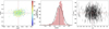 |
Fig. 1. Illustration of our Leo I data set. The left panel shows the spatial distribution of the stars, colour-coded by velocity. The middle panel shows the metallicity distribution; the mean metallicity for the galaxy is shown (black curve). The right panel shows the radial velocities as a function of right ascension, which closely corresponds to the major axis of the galaxy. |
The middle panel shows the metallicity distribution and a Gaussian fit with a mean of [Fe/H] = −1.498 dex and a standard deviation of σFe/H = 0.346 dex. Using the MCMC method we calculate a mean [Fe/H] = −1.48 ± 0.01 dex with a standard deviation of σFe/H = 0.27.
Finally, the right panel shows all measured vLOS along the α-axis centred in α2000 = 152.1146 showing a mean heliocentric velocity of the dSph galaxy, calculated with the MCMC method, of vhel = 285.2 ± 0.3 km s−1. We measure a velocity dispersion of σ = 9.2 ± 0.2 km s−1. With this we calculate the mass contained within the half-light radius using the formula from Wolf et al. (2010), valid for dispersion-supported stellar systems in dynamical equilibrium. Using the half-light radius R1/2 = 244 ± 2 pc measured by Muñoz et al. (2018), following a Sersic profile, gives us an enclosed dynamical mass of M1/2 = 1.9 ± 0.1 × 10⁷ M⊙ which is in agreement with previous calculations.
2.2. BEACON: a software that finds chemo-kinematical patterns
The BEACON software package was developed by del Pino et al. (2017) to search for rotation patterns in resolved stellar populations. The code is publicly available1, and is free to use and modify. It is written in Python, and was created to check the results of del Pino et al. (2015), who show that the Fornax dSph galaxy contains different stellar populations with different angular momenta.
BEACON is designed to find groups of stars with similar positions, velocities, and metallicities or chemical compositions. Based on the OPTICS clustering algorithm (Ankerst et al. 1999) it searches in a given data set for groups of stars with similar chemical composition and velocities, and if the number of stars in the group is bigger than a minimum cluster size (MCS), the code classifies them as a one-side stream (OSS). If on the opposite side of the centre of mass (CM) there isi a stream with similar chemical composition, but with opposite velocity, then the two groups are classified as a both-side stream (BSS) or circular stream. The full description and clustering process is described in del Pino et al. (2017), their Sect. 3.
Apart from the observational data, we needed some galaxy parameters and clustering parameters in order to create a reference frame centred on the CM of the galaxy and to control the clustering process. The galaxy parameters are the coordinates of the CM and the vhel of the CM, which are necessary to detect rotation patterns in the galaxy. The clustering parameters, on the other hand are a collection of parameters defining the clustering criteria: the standardization method and the standardization weight, the uniqueness of solution, the maxima ratio, and the inimum cluster size (MCS).
The standardization method and the standardization weight are used for the standardization of the state vector, which affect the relative importance of each coordinate during the clustering. Depending on the uniqueness of solution, BEACON can merge clusters that share stars into one cluster, thus avoiding duplicate stars, i.e., considering clusters different if they differ in at least one star. The maxima ratio is the reachable distance ratio; the higher the maxima ratio is, the more sensitivity BEACON has, making it prone to spurious detections. The minimum cluster size (MCS) is the minimum number of stars that a cluster should have to be considered a stream during the clustering process.
All these parameters have to be tuned for the specific galaxy under study and/or the scientific case, and depend on the number of sampled stars and on the completeness of the sample and its spatial coverage. We use the parameters given in Table 1 and use MCS as a parameter we vary. We give a stronger weight to the metallicity in our study as we want to compare the observations mainly to the dissolving star cluster model in which we expect the stars in one cluster to have a similar metallicity. In addition, the weight on the two coordinates is higher, as it is in studies where the authors are searching for an overall rotation pattern.
Clustering parameters: Input values for BEACON used in this work.
In previous studies the weights on positions and metallicities were lower as the authors were searching for an overall rotation pattern in the data. If we expect a rather flat rotation curve (as seen in dSph galaxies in the velocity dispersion versus radius results), it is possible to enhance the signal by placing less weight on the positions. Furthermore, expecting that the rotation is being supported by stars from different populations or at least different star-forming events, placing a weight on the metallicities would be counterproductive and make the detection much more difficult.
In contrast, when trying to find evidence for the dissolving star cluster scenario (DSCS), this choice of parameters will not work at all and will lead to a much higher rate of false detections. In the DSCS we expect each possible stream to stem from the dissolution of a small star cluster or association, formed inside the central region of the dwarf galactic DM halo; in other words, the stars should not only have similar velocities, but should also be coherent in space and have the same metallicity. Such streams are meanwhile found in our MW in the recent Gaia data catalogues. Only when placing weights on positions and metallicity do such structures become visible. On the other hand, our choice of weights does not inhibit the detection of a grand design rotation, it is just more difficult to find within the noise. The destroyed dwarf disc models we introduce at the end of our manuscript show that we are in fact able to recover an overall rotation pattern as well.
2.3. Mock data
To be able to compare our observational results with purely randomized mock data, we constructed two types of data sets that have no streaming motion.
The first type of data set represents a Plummer sphere with a Plummer radius equal to the half-light radius of Leo I. The Plummer mass is chosen to obtain a velocity dispersion similar to that of Leo 1 (i.e., the sphere is in virial equilibrium), but has no sign of rotation or any streaming motion. From the distribution function we construct 1000 samples of 1000 radial velocities. To these sets of ‘exact’ data we add random errors according to the observational uncertainties of our Leo I data.
As a second type we constructed data sets based on a similar Plummer distribution, but taking the shape of Leo 1 into account (i.e., the same eccentricity as Leo 1). The velocities are corrected as if a DM halo is present, as implied by the observations, but having no rotation or streaming motions. This model is not in equilibrium by itself, but is the closest mock representation of Leo 1 without actual rotation or streaming motion. Again, we draw 1000 samples of 1000 radial velocities from the resulting distribution function and convolve the data sets with the observational errors.
This procedure is statistically equivalent to analysing 1000 data sets of 1000 different objects (i.e., dSph galaxies) with similar parameters.
2.4. Simulations
In this study we focus on the dissolving star cluster model, as described in Assmann et al. (2013a,b), and Alarcón Jara et al. (2018). We use simulations with 16 star clusters (SCs), placed in a cusped DM halo following a Navarro Frenk and White (NFW) profile (Navarro et al. 1997) with a scale length of rs = 1 kpc, modelled with 1 000 000 particles and an enclosed mass at 500 pc of M500 = 107 M⊙. For the 16 star clusters, we adopt a SFE = 20%, amounting to a final total mass of stars Mstars = 4.5 × 10⁵ M⊙. Each star cluster itself is modelled using 100 000 particles, following a Plummer distribution with a Plummer radius of rsc = 4 pc.
The star clusters are inserted into the simulation according to a constant star formation history, as described in Alarcón Jara et al. (2018; i.e., forming one star cluster every 625 Myr). For simplicity, we assign a metallicity to each star cluster following a linear age-to-metallicity ratio given by
![Mathematical equation: $$ \begin{aligned}{[\mathrm{Fe/H}]} = -0.0004 \cdot \mathrm{Age[Myr]} + 0.3267. \end{aligned} $$](/articles/aa/full_html/2023/04/aa44209-22/aa44209-22-eq1.gif) (1)
(1)
The initial positions and velocities of the star clusters are randomly drawn from a Plummer distribution to ensure that more clusters are inserted in the central area than in the outskirts of the DM halo. The velocities are corrected for the presence of the DM halo to keep the orbit of the SCs the same as without the DM halo.
The simulations are carried out using the particle-mesh code SUPERBOX (Fellhauer et al. 2000). For more details about the initial conditions and the simulations carried out, we refer to the previous study of Alarcón Jara et al. (2018). After the simulations we add randomly drawn errors to the exact values given by the final simulation data (i.e., to the radial velocities and metallicities of our ‘stars’) according to the mean errors of our Leo I sample which are ±2.5 km s−1 and ±0.2 dex.
In these models the star clusters orbit the centre of the dark matter halo while they dissolve leaving streams of stars that conserve their kinematic properties. This is the main prediction of this model, which could be corroborated with spectroscopic observations. Examples of these rotating patterns are shown in the left panels of Fig. 2, which show their positions and velocities. To produce Fig. 2 a larger sample of particles from each SC is used (i.e., 7000 per SC) to better present the qualitative behaviour than in the subsequent analysis and to ease comparison of the different data sets.
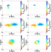 |
Fig. 2. Shapes of streams produced by dissolving star clusters in the dissolving star cluster model. The panels in the left column show all particles of a single star cluster in the chosen sample, while the right column includes only the stars of the same star cluster that are recovered and flagged as a stream by BEACON. The top row shows a recently dissolved cluster recovered by BEACON as a one-side stream. The middle row illustrates a cluster orbiting mainly in the x − z plane. The bottom row shows a cluster orbiting mainly in the x − y plane. BEACON recovers the main feature of the one-side stream of the recently dissolved cluster. It also recovers the both-side streams of the two other clusters independent of the orbital orientation. It is clear that BEACON has problems recovering the stars in the central region, which do not have large velocity differences. This behaviour is caused by the relatively large weights for the spatial coordinates. |
The first panel shows a young star cluster that is not entirely dissolved, but is in the process of dissolution; after a few hundred million years more its stars will be dispersed around the galaxy. The second and third panels show the stars for clusters that spread their stars completely around the dark matter halo, it is clear to see the streaming motion in these cases. Most of the stars with positive velocities are on one side of the dark matter halo; on the opposite side we see the stars with negative velocities.
The right panels show the stars that BEACON is able to recover for each stream. We can see that it has difficulty detecting the stars in the centre as they have relative velocities close to zero and their positions are far from the stars that have similar velocities. The lack of sensitivity in the centre can be corrected by setting a smaller weight for the radial coordinate of the stars. This would allow BEACON to find more radially distributed groups, but it could also negatively impact the purity of the resulting detected clusters.
To compare the data sets from the simulations with our observational data, we took 62 random particles from each star cluster, which gave us 992 particles in total for each set. This means that each simulated data set has an amount of stars that is similar to our observational data set.
3. Results
3.1. Simulations
It is a very difficult task to correctly recover all stars of all streams, especially once we add errors similar to the observational data. Instead of sharp metallicity peaks, we have smeared out distributions which might even overlap. In the same spatial region we might have stars from different dissolved star clusters but with very similar radial velocities. To understand better the efficiency of BEACON we define three parameters: F1, F2, and F3.
F1 is the fraction of recovered stars. We count all that stars that BEACON attributes to the different streams it finds. We divide this number by the total number of stars. F2 is the fraction of correct stars (recovered). We only count the stars that BEACON has assigned to the correct stream, and divide this number by all recovered stars. F3 is the fraction of correct stars (all). We count all correctly assigned stars, but now divided by the total number of stars. As in our simulations, all stars of the dwarf galaxy originate in streams; the division by all stars also implies the ratio of stars with respect to all stars originating in streams as well.
In Fig. 3 we plot these three fractions as a function of the clustering parameter MCS. All other values are kept constant at the values given in Table 1. We take the data sets from the three simulations of the dissolving star cluster model. This gives results with their respective error margins.
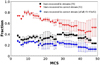 |
Fig. 3. Fractions of recovered stars as functions of the clustering parameter MCS (all other parameters are kept constant, as shown in Table 2). We show as F1 the fraction of stars assigned to streams as black squares. As F2 we show the fraction of correctly assigned stars in relation to the recovered stars. Finally, as F3 we show the fraction of correctly recovered stars compared to all stars as blue circles. We see that BEACON is indeed able to recover about 20–25% of stars as belonging to streams correctly, even though the data is degraded by errors similar to those in the observational data. |
The black squares show the fraction of stars that are assigned to streams. This fraction is constant at 40% as long as MCS is well below our sample size of 62 stars from each cluster. As soon as MCS gets closer to our sample size, this value drops.
We can see that this is not the full story if we look at the red triangles, which record the fraction of correctly assigned stars. Here we see a fraction of 70–80% of stars assigned to streams that actually belong to that stream, especially at MCS values below 20. Once we raise this parameter further this fraction drops to about only half of the recovered stars.
Finally, and most importantly, the blue dots give us the fraction of stars that are correctly assigned to their streams of all the stars in the sample. This fraction is of the order of 20–25% for small MCS values and drops below 20% if MCS gets closer to the sample size.
This in turn means that even in simulations where we should be able to recover all possible streams, once we restrict ourselves to an overall sample of about 1000 stars and adding observational errors to our data, we can only expect to recover about one-fourth of the stars correctly. This could mean, in the worst case scenario, that we might be missing the detection of three-fourths of the streams actually present in the data. This is not seen in our samples based on simulated streams, where we detect about 70% of the actual streams (see below). These values give us confidence that we can use BEACON on an observational data set and that we will obtain a sufficiently good answer; in other words, that we are able to see about a quarter of the stars assigned to their correct streams if there are any.
In Fig. 4 we show some examples of recovered streams by BEACON for one of the simulations using MCS = 10. The left panels show the positions of the stars with a colour bar for the velocities, the coloured stars are the stars that belong to the same star cluster, and the black dots are the rest of the stars in the simulated galaxy. The black arrows show the direction of the projected angular momentum. It is clearly that the stars from the same dissolved star cluster follow similar orbits since the stars with positive velocities are located at one side of the centre of the galaxy, and on the opposite side are the stars with negative velocities. The middle panels show on the x-axis the distance to the centre and on the y-axis vz the velocities. Black dots are the stars of the dissolved star cluster and red dots are the stars that BEACON recovers as a stream. We can see that BEACON recovers a large part of the stars from the sample, but a few of them were missed or misclassified. In addition, some stars from other star clusters are misclassified as members of a particular stream. In the right panels we show the particles recovered by BEACON and the stars that belong to the same star cluster. In these examples BEACON was able to recover most of the stars which show a strong rotation signal, with a few false detected stars that do not belong to the star cluster. We can see that there are a small mismatches between the projected angular momentum recovered and the real value, due to the missed stars.
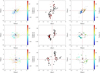 |
Fig. 4. An example of how BEACON can extract substructures hidden in a large data set with 992 particles. Here we apply BEACON to a simulation of dissolving star clusters with 16 star clusters and a constant star formation. The left panels show the position of the stars and the velocities along the z-axis are shown as colours for the stars that were formed in the same star cluster. The black triangles show the projected angular momentum direction and black dots are all other particles from the simulation. Middle panels show the velocities along the line of sight taking as a new y-axis the projected angular momentum direction, black dots are the values for the stars which belong to the same star cluster and red dots are the stars recovered by BEACON. In the right panels we show the particles recovered by BEACON in colour and in black the stars which belong to the same star cluster. In these examples BEACON was able to recover most of the stars which show a strong rotation signal, with a few false detected stars which do not belong to the star cluster. |
3.2. Comparison with mock data
As a next step we want to check how significant our detection of streams is in comparison to mock data, which by design contains no streaming motion whatsoever.
We construct samples of stars from our simulations and from the mock data of non-rotating Plummer spheres and the fake Leo I data. The size of the samples is the same as the number of observed stars we have. To the exact data we add the observational errors determined for our Leo I data set. Now BEACON is applied, keeping the parameters shown in Table 1 constant and varying the sensitivity by varying the parameter MCS. The results are shown in Fig. 5.
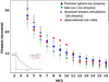 |
Fig. 5. Number of streams recovered with BEACON as a function of MCS. The blue rectangles are mean numbers taken from three simulations of the dissolving star cluster model consisting of 16 streams. The black triangles (up pointing) are for a Plummer sphere distribution with no rotation patterns (i.e., no streams); the green triangles (down pointing) are Leo I fake data, also with no streams. The red circles are the results of BEACON applied to the observational data set of the Leo I dSph. We use 2 as the value for the weight of the metallicity, with a sensitivity of 0.85 and a change in the minimum cluster size MCS. The inset shows qualitatively how a few real streams should appear in a ‘sea’ of false detections. |
The black and green triangles show the detected streams in the mock data, which by construction does not contain any streams. We can see clearly that the number of false detections decreases exponentially with decreasing the sensitivity (i.e., requiring more stars for the stream detection; increasing MCS). Error bars to these values are possible, as we construct 1000 samples of mock data.
The blue squares show the number of detected streams in our dissolving star cluster simulations, consisting of 16 different star clusters. We use three different samples from three different simulations to be able to place error bars on the measured values.
If we used the exact data of one sample, which would allow the detection of all streams, we would expect a curve in which for small MCS the real detections would be surpassed by the noise of false detections. Once the false detections fall below the number of real detectable streams, the data points should show an almost constant value as function of MCS (i.e., the real streams plus some small contribution of the noise). Once MCS reaches the sample size of the stars belonging to a stream, the detection signal should go rapidly back to the noise level (see inset of Fig. 5).
As we are using multiple samples from different simulations, we cannot expect such a curve. Instead, we have to deal with a super-position of a multitude of such curves, smearing out this clear signal. Even so, we see that as soon as we require an MCS > 8, the blue symbols are always above the curves of false detections. The blue symbols should fall back down within the noise level once we reach MCS values close to about 20% of the actual sample size (i.e., stars drawn from that particular dissolved cluster) as we expect only to recover about 20–25% of the stars from a stream correctly (see Fig. 3). The red circles are based on the observational data of Leo I which we talk about in the next section.
Unluckily, the small sample size of fewer than a thousand stars combined with the observational uncertainties leads to overlapping error bars; the real detections of streams are not above the noise level by a statistically significant amount.
3.3. Observational results
In Fig. 5 the black and green triangles represented the mock data. In an ideal world we would like the response of BEACON to be zero. This is not the case, and if we reduce the sensitivity of BEACON such that we get an almost zero response in the no-stream data sets, we also get a similar response for the simulation data, where streams are clearly present (blue squares). For very high sensitivities the response of BEACON gives us more streams than are actually in the data.
To analyse the observational data of Leo I we require that BEACON does not recover more streams than are actually present for the dissolving star cluster data (i.e., 16 streams for the blue symbols). Furthermore, we want the false detection (green and black) to be below the number of streams detected in the real observational data (red dots). These requirements are matched using a MCS range between 8 and 11.
Furthermore, we note that the red data points follow that pattern that we predict theoretically in Sect. 3.2. This could be a clear sign that there is actually detectable streaming motion present in the observational data of Leo I.
For the further analysis we apply a MCS parameter of 10. With this value we find 14 detections of probable streams with BEACON. At MCS = 10 we find 11 ± 2 streams out of 16 in our simulations of the dissolving star cluster model, and we can calculate the probability of finding 14 or more streams in the mock data, which is as low as 1.7% in the case of the Plummer sphere data and just 0.4% in the case of Leo I mock data, making it a statistically significant detection.
In Fig. 6 we show some examples of the streams detected in the observational sample of Leo I. The left panels show the positions of all measured stars as black dots; the stars recovered as a stream are coloured according to their radial velocities. The black arrows show the direction of the projected angular momentum. In the middle panels the radial velocities as function of the distance to the centre are shown, and in the right panels the metallicity distribution of all measured stars in red and the metallicities of the recovered stars of that particular stream as black histograms. The fact that ≈40% of the stars were classified in a stream is in agreement with the values recovered by BEACON in a simulation with 16 star clusters using the same parameters (see Fig. 3, where the black boxes indicate the fraction of stars recovered in a simulation of the dissolving star cluster model: ≈35%).
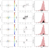 |
Fig. 6. Examples of stream motions recovered by BEACON in the observational data of Leo I. Left panels: positions of all observed stars as small black points. The coloured points are the stars BEACON joins to a stream detection; the colour represents the radial velocity measured for each star. The direction of the projected angular momentum of this stream is shown as a black arrow. Middle panels: radial velocity of the stars belonging to the stream as a function of their distance to the centre of the dwarf galaxy. Right panels: Metallicity distribution of the whole sample (red) and the metallicity distribution of the stars from the stream recovered by BEACON (black). |
No OSS is detected by BEACON in Leo I. The sample of stars used in this work consider just RGB stars that are older than 2 Gyr, so they would have enough time to be dispersed around the galaxy to show up as a BSS.
After applying BEACON to our catalogue with input parameters shown in Table 1 a total of 406 stars were classified into 14 possible circular streams. The other stars were considered as stars that do not follow any strong chemo-kinematical pattern. Some of these stars may belong to rotating streams and may have been misclassified, as in the simulations. Some stars show nearly zero vLOS, making their classification into BSSs difficult. Some others may simply belong to poorly sampled populations that have not fulfilled the minimum requirements to be considered as a group. Given the fraction of correctly recovered stars in the simulated data (F3), these results are consistent with most or all of the Leo I stellar population originating in clusters that have now dissolved, spreading their stars inside the DM halo of the dSph, but still following orbits similar to their original SC.
Table 2 shows the properties of the 14 streams recovered by BEACON. The projected angular momentum can be derived for each BSS,  , where mi is the mass of the ith star and j is the number of stars in the BSS. A priori, we do not have information about the homogeneity of our sample in terms of metallicity. A sensible way to avoid sampling effect is to normalize the L vector of every group to the number of stars in the group. This is roughly the same as expressing the angular momentum per unit of stellar mass and provides a measure of the mean momentum p of the stars forming a BSS. In the following we use only quantities normalized in this way.
Parameters from the BSS recovered by BEACON in Leo I.
The question arises of why, in Table 2, all streams show member counts of 19 and more, while the red data points of recovered streams as function of MCS disappears into the noise already at values equal to 12. This is due to the fact that BEACON after a first detection (using MCS) is searching for more stars that could belong to the stream, and is also grouping similar streams together. Finally, once a OSS is detected, it searches on the other side of the galaxy for a counterpart to combine into a BSS. As stated above, all recovered streams in the Leo I data are BSSs.
3.4. Some caveats
As a final test we vary the mean heliocentric velocity vhel of Leo I in the application of BEACON on our observational data. As shown before, streams with velocities almost perpendicular to the line of sight, as well as stars in a stream close to the centre of the dwarf with relative velocities close to zero, are undetectable by BEACON. So we expect the detection of some streams to be highly dependent on the correct choice of the mean velocity of Leo I. The results of this test are shown in Fig. 7.
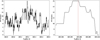 |
Fig. 7. Number of recovered streams using MCS = 10 vs. the mean heliocentric velocity of Leo I vhel. Left panel: we apply BEACON varying the vhel = 285.2 between ±0.31 with steps of 0.0001 km s−1. The maximum number of streams is recovered between 285.196442 < Vhel < 285.199738 km s−1. Right panel: magnified image of the central region shown in the left panel. The adopted Vhel = 285.1994 km s−1 in our study is shown as a red vertical line. |
Both panels of the figure show the number of recovered streams as a function of the mean heliocentric velocity, which we have used in BEACON as a fixed parameter so far. The right panel is a zoomed-in image of the central part of the left panel. We see strong variations in the number of recovered streams when changing the adopted velocity by just a few metres per second; the maximum number is at the determined systemic velocity of Leo I.
We can read the results in two fashions. First, the choice of the mean velocity is much more important than we believed before and the number of detected streams drops significantly by changing the velocity by just 0.01 km s−1, while the errors of every single velocity measurement is of the order of 2.5 km s−1. Because BEACON is based on OPTICS, which is a purely geometrical clustering algorithm, changing the velocity by just 0.01 km s−1 can change the way clusters are built. This could cause some groups to change their member stars and to not fulfil the MCS and the maxima ratio conditions, and thus to stop being considered by BEACON as a group.
The second interpretation is that we see the influence of the randomness of the false detections. This would make the 14 detections in our study just outliers; a more correct result, looking at the variations of detected streams, would be 10 ± 3 streams. This would place our result still above the data points from the pure noise false detections, but with strongly overlapping error bars, similar to the calculated mean value from our simulations of the dissolving star cluster models.
Our general result would still stand that the observational data of Leo I is in agreement with the DSCM, but with not enough real streams to have a detection that is significantly above the noise of having no coherent motion at all. More data with smaller observational errors would be necessary to validate or reject this particular formation scenario for Leo I.
3.5. Tidal stirring model
Figure 8 (left panel) shows the projected angular momentum L of the 14 streams recovered by BEACON compared with the 16 streams of a simulation of the dissolving star cluster model (middle panel). According to the dissolving star cluster model the projected angular momentum is randomly distributed in the galaxy, as shown in Fig. 8. The presence of these streaming motions could be a hint to corroborate our model of the formation of dwarf spheroidal galaxies.
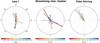 |
Fig. 8. Angular momentum per unit of stellar mass for different streams. Left panel: different angular momentum patterns recovered by BEACON in the 14 streams of the sample of 953 stars from Leo I, coloured according to their [Fe/H]. Middle panel: angular momentum for a simulation of the dissolving star cluster model with 16 star clusters dissolved. Circles have radius from 0 pc2 s−1 to 3 × 10³ pc2 s−1 with step of 0.5 × 10³ pc2 s−1 for each dotted concentric circle. Right panel: angular momentum of the streams recovered by BEACON in a tidal stirring simulation. There is no net rotation signal in the Leo I observational data and in the dissolving star cluster model, while in the tidal stirring model the angular momentum vectors point in roughly the same direction, suggesting a remnant rotation signal. |
Finally, we performed N-body simulations of the tidal stirring and ram pressure model (Mayer et al. 2007), in which a small disc galaxy is orbiting a large galaxy like our Milky Way and gets distorted via ram pressure and tidal stirring. Ram pressure removes the gas from the dwarf and tidal stirring destroys the stellar disc and parts of the DM halo. We use the code GADGET2 (Springel 2005) to run simulations of the tidal stirring model using the same set-up as Mayer et al. (2007). We vary the initial distance of the disc galaxy to mimic the formation of a dSph galaxy like Leo I. More details of the set-up will be presented in Alarcon et al. (in prep.).
Preliminary results of the simulations show that after 10 Gyr of evolution the final objects can have properties that are similar to those of the observed dwarf spheroidal galaxies. For example the spherical shapes, exponential surface brightness profiles, and high velocity dispersion values which remain constant independent of the distance from the centre, as predicted by the model. Applying BEACON with the same parameters used in our analysis of Leo I, selecting the same number of stars, and giving the same metallicity distribution of Leo I to the particles, we can see that the final object still has a remnant rotation signal that BEACON is able to recover (see Fig. 8, right panel).
The strength of this remnant rotation is highly dependent on the number of orbits around the large galaxy, but if the disc galaxy is far from its host it will not be able to lose its rotation completely. We can see in the right panel of Fig. 8 that the recovered streams are pointing in the same direction. In this simulation during 10 Gyr the disc galaxy is able to make one and a half orbits around the large galaxy, and does not have enough time to get rid of its rotation.
A detailed analysis with BEACON of simulations using the tidal stirring model will be performed in the future, and is not part of the present study. We show the right panel of Fig. 8 just to give a hint of future results.
4. Discussion and conclusions
Using BEACON to search for streaming motions arising from the Dissolving Star Cluster Model in case of perfect data (i.e., no errors and large sample sizes), almost all streams are detected. Only streaming motions almost perpendicular to the line of sight are very hard to detect. A slow rotation pattern close to the centre of the dwarf galaxy may also escape detection. In these cases the correct determination of the dwarf galaxy’s radial velocity might become crucial. Very eccentric orbits of streams might also not get grouped together because the software is searching for rotation patterns rather than any streaming motion.
False positives decline rapidly and exponentially with the required minimum cluster size (MCS), so that on perfect simulation data (see above) they do not play a role. This picture changes when adding the typical observational errors (i.e., noise) to the data and reducing the sample size dramatically. In our study we adopted a sample size of 1000 data points and similar errors to those associated with the observations of the Leo 1 data.
At small MCS, the real streams get drowned in a sea of false positives, but at one point it seems that most false positives get suppressed and surpassed by real streams. Otherwise it is not easy to explain why, in a comparison between no-stream data and pure-stream data, that we see the data points of the pure-stream data just above the no-stream data, implying that maybe just 25% of the streams present are detected and most of the detected streams are false positives. Even so, we see a detection rate of 70% of the streams present. A possible explanation could be that the algorithm includes a re-grouping of detections with similar properties (i.e., close in position and/or radial velocities). Somehow, this favours real streams over false positives.
Once MCS is increased further and gets closer to about 25% of the actual data points belonging to a real stream, the detection rate drops back into the noise level of false positives. This means there is a sweet spot or region in MCS where the number of detections is expected to be larger, if real streams are present, than the number of pure false positives would predict. This might not be on a statistically significant level, but it is visible in Fig. 5. Furthermore, in that region of parameter space more detections might be real than a simple comparison with no-stream data (i.e., pure false positive data) would imply.
Putting our results into context, we are not the first to use BEACON to search for chemo-kinematical patterns in dSph galaxies. del Pino et al. (2017) use BEACON to search for chemo-kinematical patterns in the Fornax dSph galaxy using 2562 stars from different catalogues (Pont et al. 2004; Battaglia et al. 2006, 2008; Walker et al. 2009; Kirby et al. 2010; Letarte et al. 2010). We made a similar analysis using data from Leo I, with a total of 953 stars with their respective metallicity and velocity values along the line of sight taken from the Keck and Magellan Telescopes. A direct comparison of the results of the two studies are strikingly similar.
del Pino et al. (2017) found that approximately 40% of the stars may be part of different substructures, with 985 stars classified into 24 possible circular streams using a MCS = 13. This could indicate that Fornax is a rather complex system with various rotating components and its spheroidal shape is the superposition of stellar components with distinct kinematics (see their Fig. 13). In our study we find 14 possible streams in Leo I, consisting of about 40% of all stars in our sample.
If we compare our Fig. 5 with their Fig. 5 we clearly see the same exponential decrease in false detections as we have proven with our mock data. In their analysis we can see the same signal of possible real streams above the noise level at values of MCS between 20 and 35. In their Fig. 6 we see a peak similar to the one in our Fig. 7, even though they use a much coarser grid of possible velocities as they check for the 2D position of the galaxy centre as well.
The star formation history of Fornax together with the spatial distribution of its stars and their kinematics suggest that Fornax could be the remnant of a merger between two small galaxies that collided and merged to form the dSph we observe today (Alarcón Jara et al. 2018; del Pino et al. 2015, 2017). Apart from SFH or chemistry, the kinematic features that are similar to those observed in Fornax could be explained by the dissolving star cluster model without the necessity of a merger history (see their Figs. 9 and 15 and compare them with our Fig. 8).
We compare the observational results to mock data deliberately designed to not show any rotation or streaming signal, to assess the level of possible false detections in a given data set. Unluckily, the size and accuracy of the present-day data may not allow us to obtain streaming motion signals that are statistically significant beyond any doubt.
We find multiple rotating populations in Leo I with random orientation of the projected angular momentum, which could indicate that the overall structure of dSph galaxies is due to the superposition of different stellar populations with different streaming orbits, as predicted in the dissolving star cluster model. The amount of stars (about 40%) we find to belong to streaming motions is in agreement with all stars belonging to streams of dissolved star clusters.
In the context of this model, these chemo-kinematic patterns are one of the main predictions as explained and demonstrated in Assmann et al. (2013a,b), and Alarcón Jara et al. (2018) and come naturally with this model. However, these patterns could be explained by other models assuming rotating progenitors (e.g. the tidal stirring model), which explains the formation of dSph as interactions between a disc galaxy and a MW size galaxy as well. These interactions could be responsible for the reshaping of the disc galaxy into a dSph (Mayer 2010). Simulations show that after a significant time the final object conserves some signatures of this process and could have remnant rotation around the minor axis.
Another option to explain these patterns is invoking that the evolution of dSph galaxies could involve several mergers between two or more smaller galaxies. In these models two disc galaxies collide, and as a result they could form a dSph galaxy. This has been studied before, and shows that some of the orbits of stars of the progenitors could remain after the collision (Amorisco & Evans 2012).
Cicuéndez & Battaglia (2018) made an analysis of the chemical composition and velocities of stars from the Sextans dSph and have shown that there are two different populations that have chemo-kinematic patterns that could be a sign of a past material accretion. They reported a shell structure for young stars and a ring-like structure for older stars. Karlsson et al. (2012), Kim et al. (2019), and Aoki et al. (2020) analysed the data of the Sextans dSph as well, and think they have found the streaming motion of a dissolved star cluster.
These publications show that the analysis of chemo-kinematical patterns is indeed possible with modern data sets, even though our study has shown that the results may not yet be as statistically convincing as we would like. Nevertheless, it shows a clear pathway of how the large data sets that we have today and the much larger data sets of the future should be analysed.
We have explained the theoretical pattern a given streaming signal should have when appearing above a given noise level of false detections. This kind of pattern is clearly visible in our study and in the previous work of del Pino et al. (2017). This pattern cannot be explained by pure noise and is for us a clear sign that there is a streaming motion present in Leo I. We hope with future observations that the signal will become stronger and be significantly above the noise level. The fact that it is present in two different dSph galaxies and two independent studies is more than promising.
Furthermore, thanks to a rigid comparison with mock data having no streaming motions and simulations built up by only streams, we have shown that the number of streams we detect is unlikely to be from a data set without any streaming motion at a 98–99% level of confidence. Therefore, even though we cannot tell for certain which of our detections is based on a real stream and which not, the evidence points to the presence of streaming motion in the observational data.
In order to have a better understanding of the origin of dSph galaxies, it is necessary to apply BEACON to other dSph galaxies for which high quality data sets are available in order to search for chemo-kinematical substructures in those systems to be able to distinguish between the different formation scenarios for dSph galaxies (Diemand et al. 2008; Hamuy et al. 1996; Koposov et al. 2009; Łokas et al. 2008; Olszewski et al. 1996; Perlmutter 1999; Riess et al. 2004; Spergel 1993; Tolstoy et al. 2009; Lora et al. 2019; Valenzuela et al. 2007; van den Bergh & Herbst 2000; McConnachie et al. 2010).
We show that Leo I and Fornax (del Pino et al. 2017) were very likely formed by the superposition of different stellar components, rotating in the galaxy with projected angular momentum pointing in different directions. This result is in agreement with the dissolving star cluster model.
Acknowledgments
A.A. acknowledges financial support from Carnegie Institution for Science with its Carnegie-Chile Fellowship, Fondecyt regular No. 1180291 and Centro de Astrofisica y Tecnologias Afines (CATA) grant PFB-06/2017. M.F. acknowledges funding through Fondecyt regular No. 1180291, Conicyt PII20150171, Quimal No.170001 and the ANID BASAL projects ACE210002 and FB210003. A.d.P. acknowledges the financial support from the Spanish Ministry of Science and Innovation and the European Union – NextGenerationEU through the Recovery and Resilience Facility project ICTS-MRR-2021-03-CEFCA. We thank Marla Geha for providing the stellar velocities from the Keck/DEIMOS data set. The data underlying this article will be shared on reasonable request to the corresponding author.
References
- Alarcón Jara, A. G., Fellhauer, M., Matus Carrillo, D. R., et al. 2018, MNRAS, 473, 5015 [CrossRef] [Google Scholar]
- Amorisco, N. C., & Evans, N. W. 2012, ApJ, 756, L2 [NASA ADS] [CrossRef] [Google Scholar]
- Ankerst, M., Breunig, M. M., Peter Kriegel, H., & Sander, J. 1999, OPTICS: Ordering Points To Identify the Clustering Structure (ACM Press), 49 [Google Scholar]
- Aoki, M., Aoki, W., & François, P. 2020, A&A, 636, A111 [NASA ADS] [CrossRef] [EDP Sciences] [Google Scholar]
- Assmann, P., Fellhauer, M., Wilkinson, M. I., & Smith, R. 2013a, MNRAS, 432, 274 [NASA ADS] [CrossRef] [Google Scholar]
- Assmann, P., Fellhauer, M., Wilkinson, M. I., Smith, R., & Blaña, M. 2013b, MNRAS, 435, 2391 [CrossRef] [Google Scholar]
- Battaglia, G., Tolstoy, E., Helmi, A., et al. 2006, A&A, 459, 423 [NASA ADS] [CrossRef] [EDP Sciences] [Google Scholar]
- Belokurov, V., Zucker, D. B., Evans, N. W., et al. 2007, ApJ, 654, 897 [Google Scholar]
- Battaglia, G., Helmi, A., Tolstoy, E., et al. 2008, ApJ, 681, L13 [NASA ADS] [CrossRef] [Google Scholar]
- Bosler, T. L., Smecker-Hane, T. A., & Stetson, P. B. 2007, MNRAS, 378, 318 [NASA ADS] [CrossRef] [Google Scholar]
- Boylan-Kolchin, M., Bullock, J. S., Sohn, S. T., Besla, G., & van der Marel, R. P. 2013, ApJ, 768, 140 [NASA ADS] [CrossRef] [Google Scholar]
- Bustamante-Rosell, M. J., Noyola, E., Gebhardt, K., et al. 2021, ApJ, 921, 107 [NASA ADS] [CrossRef] [Google Scholar]
- Cicuéndez, L., & Battaglia, G. 2018, MNRAS, 480, 251 [CrossRef] [Google Scholar]
- Cole, S., Aragon-Salamanca, A., Frenk, C. S., Navarro, J. F., & Zepf, S. E. 1994, MNRAS, 271, 781 [NASA ADS] [CrossRef] [Google Scholar]
- del Pino, A., Aparicio, A., & Hidalgo, S. L. 2015, MNRAS, 454, 3996 [NASA ADS] [CrossRef] [Google Scholar]
- del Pino, A., Łokas, E. L., Hidalgo, S. L., & Fouquet, S. 2017, MNRAS, 469, 4999 [Google Scholar]
- Diemand, J., Kuhlen, M., Madau, P., et al. 2008, Nature, 454, 735 [NASA ADS] [CrossRef] [Google Scholar]
- D’Onghia, E., Besla, G., Cox, T. J., & Hernquist, L. 2009, Nature, 460, 605 [CrossRef] [Google Scholar]
- Dressler, A., Hare, T., Bigelow, B. C., & Osip, D. J. 2006, Proc. SPIE, 6269, 62690F [NASA ADS] [CrossRef] [Google Scholar]
- Faber, S. M., Phillips, A. C., Kibrick, R. I., et al. 2003, Proc. SPIE, 4841, 1657 [NASA ADS] [CrossRef] [Google Scholar]
- Fellhauer, M., Kroupa, P., Baumgardt, H., et al. 2000, New Astron., 5, 305 [NASA ADS] [CrossRef] [Google Scholar]
- Gaia Collaboration 2018, VizieR Online Data Catalog: I/345 [Google Scholar]
- Gallart, C., Freedman, W. L., Aparicio, A., Bertelli, G., & Chiosi, C. 1999, AJ, 118, 2245 [NASA ADS] [CrossRef] [Google Scholar]
- Gnedin, O. Y., Hernquist, L., & Ostriker, J. P. 1999, ApJ, 514, 109 [NASA ADS] [CrossRef] [Google Scholar]
- Grcevich, J., & Putman, M. E. 2009, ApJ, 696, 385 [NASA ADS] [CrossRef] [Google Scholar]
- Gullieuszik, M., Held, E. V., Saviane, I., & Rizzi, L. 2009, A&A, 500, 735 [NASA ADS] [CrossRef] [EDP Sciences] [Google Scholar]
- Hamuy, M., Phillips, M. M., Suntzeff, N. B., et al. 1996, AJ, 112, 2391 [Google Scholar]
- Harrington, R. G., & Wilson, A. G. 1950, PASP, 62, 118 [NASA ADS] [CrossRef] [Google Scholar]
- Hernandez, X., Gilmore, G., & Valls-Gabaud, D. 2000, MNRAS, 317, 831 [CrossRef] [Google Scholar]
- Hodge, P. W. 1962, AJ, 67, 125 [NASA ADS] [CrossRef] [Google Scholar]
- Karlsson, T., Bland-Hawthorn, J., Freeman, K. C., & Silk, J. 2012, ApJ, 759, 111 [Google Scholar]
- Kauffmann, G., White, S. D. M., & Guiderdoni, B. 1993, MNRAS, 264, 201 [Google Scholar]
- Kim, H.-S., Han, S.-I., Joo, S.-J., Jeong, H., & Yoon, S.-J. 2019, ApJ, 870, L8 [NASA ADS] [CrossRef] [Google Scholar]
- Kirby, E. N., Guhathakurta, P., Simon, J. D., et al. 2010, ApJS, 191, 352 [NASA ADS] [CrossRef] [Google Scholar]
- Kirby, E. N., Lanfranchi, G. A., Simon, J. D., Cohen, J. G., & Guhathakurta, P. 2011, ApJ, 727, 78 [Google Scholar]
- Kleyna, J., Wilkinson, M. I., Evans, N. W., Gilmore, G., & Frayn, C. 2002, MNRAS, 330, 792 [NASA ADS] [CrossRef] [Google Scholar]
- Kleyna, J. T., Wilkinson, M. I., Gilmore, G., & Evans, N. W. 2003, ApJ, 589, L59 [NASA ADS] [CrossRef] [Google Scholar]
- Knapp, G. R., Kerr, F. J., & Bowers, P. F. 1978, AJ, 83, 360 [NASA ADS] [CrossRef] [Google Scholar]
- Koch, A., Wilkinson, M. I., Kleyna, J. T., et al. 2009, ApJ, 690, 453 [NASA ADS] [CrossRef] [Google Scholar]
- Koposov, S. E., Yoo, J., Rix, H.-W., et al. 2009, ApJ, 696, 2179 [NASA ADS] [CrossRef] [Google Scholar]
- Lee, M. G., Freedman, W., Mateo, M., et al. 1993, AJ, 106, 1420 [NASA ADS] [CrossRef] [Google Scholar]
- Letarte, B., Hill, V., Tolstoy, E., et al. 2010, A&A, 523, A17 [NASA ADS] [CrossRef] [EDP Sciences] [Google Scholar]
- Łokas, E. L. 2009, MNRAS, 394, L102 [NASA ADS] [CrossRef] [Google Scholar]
- Łokas, E. L., Klimentowski, J., Kazantzidis, S., & Mayer, L. 2008, MNRAS, 390, 625 [CrossRef] [Google Scholar]
- Lora, V., Grebel, E. K., Schmeja, S., & Koch, A. 2019, ApJ, 878, 152 [NASA ADS] [CrossRef] [Google Scholar]
- Mateo, M. L. 1998, ARA&A, 36, 435 [NASA ADS] [CrossRef] [Google Scholar]
- Mateo, M., Olszewski, E. W., & Walker, M. G. 2008, ApJ, 675, 201 [NASA ADS] [CrossRef] [Google Scholar]
- Mayer, L. 2010, Adv. Astron., 2010, 278434P [NASA ADS] [CrossRef] [Google Scholar]
- Mayer, L., Kazantzidis, S., Mastropietro, C., & Wadsley, J. 2007, Nature, 445, 738 [NASA ADS] [CrossRef] [Google Scholar]
- McConnachie, A. W. 2012, AJ, 144, 4 [Google Scholar]
- McConnachie, A. W., Ferguson, A. M. N., Irwin, M. J., et al. 2010, ApJ, 723, 1038 [NASA ADS] [CrossRef] [Google Scholar]
- Muñoz, R. R., Frinchaboy, P. M., Majewski, S. R., et al. 2005, ApJ, 631, L137 [CrossRef] [Google Scholar]
- Muñoz, R. R., Majewski, S. R., Zaggia, S., et al. 2006, ApJ, 649, 201 [CrossRef] [Google Scholar]
- Muñoz, R. R., Côté, P., Santana, F. A., et al. 2018, ApJ, 860, 66 [CrossRef] [Google Scholar]
- Navarro, J. F., Frenk, C. S., & White, S. D. M. 1997, ApJ, 490, 493 [Google Scholar]
- Olszewski, E. W., Pryor, C., & Armandroff, T. E. 1996, AJ, 111, 750 [NASA ADS] [CrossRef] [Google Scholar]
- Perlmutter, S. 1999, HST Proposal ID 8346, Cycle 8 [Google Scholar]
- Pont, F., Zinn, R., Gallart, C., Hardy, E., & Winnick, R. 2004, AJ, 127, 840 [Google Scholar]
- Riess, A. G., Li, W., Stetson, P. B., et al. 2004, Am. Astron. Soc. Meet. Abstr., 205, 69.05 [NASA ADS] [Google Scholar]
- Simon, J. D., & Geha, M. 2007, ApJ, 670, 313 [NASA ADS] [CrossRef] [Google Scholar]
- Sohn, S. T., Majewski, S. R., Muñoz, R. R., et al. 2007, ApJ, 663, 960 [NASA ADS] [CrossRef] [Google Scholar]
- Sohn, S. T., Besla, G., van der Marel, R. P., et al. 2013, ApJ, 768, 139 [NASA ADS] [CrossRef] [Google Scholar]
- Spergel, D. N. 1993, ApJ, 412, L5 [NASA ADS] [CrossRef] [Google Scholar]
- Springel, V. 2005, MNRAS, 364, 1105 [Google Scholar]
- Tolstoy, E., Hill, V., & Tosi, M. 2009, ARA&A, 47, 371 [Google Scholar]
- Valenzuela, O., Rhee, G., Klypin, A., et al. 2007, ApJ, 657, 773 [NASA ADS] [CrossRef] [Google Scholar]
- van den Bergh, S., & Herbst, W. 2000, VizieR Online Data Catalog: VII/218 [Google Scholar]
- Walker, M. G., Mateo, M., Olszewski, E. W., et al. 2007, ApJ, 667, L53 [NASA ADS] [CrossRef] [Google Scholar]
- Walker, M. G., Mateo, M., Olszewski, E. W., et al. 2009, ApJ, 704, 1274 [Google Scholar]
- Weisz, D. R., Dolphin, A. E., Skillman, E. D., et al. 2014a, ApJ, 789, 147 [Google Scholar]
- Weisz, D. R., Dolphin, A. E., Skillman, E. D., et al. 2014b, ApJ, 789, 148 [NASA ADS] [CrossRef] [Google Scholar]
- Wolf, J., Martinez, G. D., Bullock, J. S., et al. 2010, MNRAS, 406, 1220 [NASA ADS] [Google Scholar]
All Tables
All Figures
|
Fig. 1. Illustration of our Leo I data set. The left panel shows the spatial distribution of the stars, colour-coded by velocity. The middle panel shows the metallicity distribution; the mean metallicity for the galaxy is shown (black curve). The right panel shows the radial velocities as a function of right ascension, which closely corresponds to the major axis of the galaxy. |
| In the text | |
|
Fig. 2. Shapes of streams produced by dissolving star clusters in the dissolving star cluster model. The panels in the left column show all particles of a single star cluster in the chosen sample, while the right column includes only the stars of the same star cluster that are recovered and flagged as a stream by BEACON. The top row shows a recently dissolved cluster recovered by BEACON as a one-side stream. The middle row illustrates a cluster orbiting mainly in the x − z plane. The bottom row shows a cluster orbiting mainly in the x − y plane. BEACON recovers the main feature of the one-side stream of the recently dissolved cluster. It also recovers the both-side streams of the two other clusters independent of the orbital orientation. It is clear that BEACON has problems recovering the stars in the central region, which do not have large velocity differences. This behaviour is caused by the relatively large weights for the spatial coordinates. |
| In the text | |
|
Fig. 3. Fractions of recovered stars as functions of the clustering parameter MCS (all other parameters are kept constant, as shown in Table 2). We show as F1 the fraction of stars assigned to streams as black squares. As F2 we show the fraction of correctly assigned stars in relation to the recovered stars. Finally, as F3 we show the fraction of correctly recovered stars compared to all stars as blue circles. We see that BEACON is indeed able to recover about 20–25% of stars as belonging to streams correctly, even though the data is degraded by errors similar to those in the observational data. |
| In the text | |
|
Fig. 4. An example of how BEACON can extract substructures hidden in a large data set with 992 particles. Here we apply BEACON to a simulation of dissolving star clusters with 16 star clusters and a constant star formation. The left panels show the position of the stars and the velocities along the z-axis are shown as colours for the stars that were formed in the same star cluster. The black triangles show the projected angular momentum direction and black dots are all other particles from the simulation. Middle panels show the velocities along the line of sight taking as a new y-axis the projected angular momentum direction, black dots are the values for the stars which belong to the same star cluster and red dots are the stars recovered by BEACON. In the right panels we show the particles recovered by BEACON in colour and in black the stars which belong to the same star cluster. In these examples BEACON was able to recover most of the stars which show a strong rotation signal, with a few false detected stars which do not belong to the star cluster. |
| In the text | |
|
Fig. 5. Number of streams recovered with BEACON as a function of MCS. The blue rectangles are mean numbers taken from three simulations of the dissolving star cluster model consisting of 16 streams. The black triangles (up pointing) are for a Plummer sphere distribution with no rotation patterns (i.e., no streams); the green triangles (down pointing) are Leo I fake data, also with no streams. The red circles are the results of BEACON applied to the observational data set of the Leo I dSph. We use 2 as the value for the weight of the metallicity, with a sensitivity of 0.85 and a change in the minimum cluster size MCS. The inset shows qualitatively how a few real streams should appear in a ‘sea’ of false detections. |
| In the text | |
|
Fig. 6. Examples of stream motions recovered by BEACON in the observational data of Leo I. Left panels: positions of all observed stars as small black points. The coloured points are the stars BEACON joins to a stream detection; the colour represents the radial velocity measured for each star. The direction of the projected angular momentum of this stream is shown as a black arrow. Middle panels: radial velocity of the stars belonging to the stream as a function of their distance to the centre of the dwarf galaxy. Right panels: Metallicity distribution of the whole sample (red) and the metallicity distribution of the stars from the stream recovered by BEACON (black). |
| In the text | |
|
Fig. 7. Number of recovered streams using MCS = 10 vs. the mean heliocentric velocity of Leo I vhel. Left panel: we apply BEACON varying the vhel = 285.2 between ±0.31 with steps of 0.0001 km s−1. The maximum number of streams is recovered between 285.196442 < Vhel < 285.199738 km s−1. Right panel: magnified image of the central region shown in the left panel. The adopted Vhel = 285.1994 km s−1 in our study is shown as a red vertical line. |
| In the text | |
|
Fig. 8. Angular momentum per unit of stellar mass for different streams. Left panel: different angular momentum patterns recovered by BEACON in the 14 streams of the sample of 953 stars from Leo I, coloured according to their [Fe/H]. Middle panel: angular momentum for a simulation of the dissolving star cluster model with 16 star clusters dissolved. Circles have radius from 0 pc2 s−1 to 3 × 10³ pc2 s−1 with step of 0.5 × 10³ pc2 s−1 for each dotted concentric circle. Right panel: angular momentum of the streams recovered by BEACON in a tidal stirring simulation. There is no net rotation signal in the Leo I observational data and in the dissolving star cluster model, while in the tidal stirring model the angular momentum vectors point in roughly the same direction, suggesting a remnant rotation signal. |
| In the text | |
Current usage metrics show cumulative count of Article Views (full-text article views including HTML views, PDF and ePub downloads, according to the available data) and Abstracts Views on Vision4Press platform.
Data correspond to usage on the plateform after 2015. The current usage metrics is available 48-96 hours after online publication and is updated daily on week days.
Initial download of the metrics may take a while.