| Issue |
A&A
Volume 665, September 2022
|
|
|---|---|---|
| Article Number | A133 | |
| Number of page(s) | 15 | |
| Section | Stellar structure and evolution | |
| DOI | https://doi.org/10.1051/0004-6361/202243959 | |
| Published online | 20 September 2022 | |
Evolution of massive stars with new hydrodynamic wind models
1
Departamento de Ciencias, Facultad de Artes Liberales, Universidad Adolfo Ibáñez, Av. Padre Hurtado 750, Viña del Mar, Chile
e-mail: This email address is being protected from spambots. You need JavaScript enabled to view it.
2
Instituto de Física y Astronomía, Universidad de Valparaíso, Av. Gran Bretaña 1111, Casilla, 5030 Valparaíso, Chile
3
Instituto de Astrofísica, Facultad de Física, Pontificia Universidad Católica de Chile, 782-0436 Santiago, Chile
4
Centro de Astrofísica, Universidad de Valparaíso, Av. Gran Bretaña 1111, Casilla, 5030 Valparaío, Chile
5
Geneva Observatory, University of Geneva, Maillettes 51, 1290 Sauverny, Switzerland
6
School of Physics, Trinity College Dublin, University of Dublin, Dublin, Ireland
Received:
5
May
2022
Accepted:
10
July
2022
Abstract
Context. Mass loss through radiatively line-driven winds is central to our understanding of the evolution of massive stars in both single and multiple systems. This mass loss plays a key role in modulating massive star evolution at different metallicities, especially in the case of very massive stars (M* ≥ 25 M⊙).
Aims. Here we present evolutionary models for a set of massive stars, introducing a new prescription for the mass-loss rate obtained from hydrodynamical calculations in which the wind velocity profile, v(r), and the line-acceleration, gline, are obtained in a self-consistent way. These new prescriptions cover most of the main sequence phase of O-type stars.
Methods. We made a grid of self-consistent mass-loss rates Ṁsc for a set of standard evolutionary tracks (i.e. using the old prescription for mass-loss rate) with different values for initial mass and metallicity. Based on this grid, we elaborate a statistical analysis to create a new simple formula for predicting the values of Ṁsc from the stellar parameters alone, without assuming any extra condition for the wind description. Therefore, replacing the mass-loss rates at the main sequence stage provided by the standard Vink’s formula with our new recipe, we generate a new set of evolutionary tracks for MZAMS = 25, 40, 70, and 120 M⊙ and metallicities Z = 0.014 (Galactic), Z = 0.006 (LMC), and Z = 0.002 (SMC).
Results. Our new derived formula for mass-loss rate predicts a dependence Ṁ ∝ Za, where a is no longer constant but dependent on the stellar mass: ranging from a ∼ 0.53 when M* ∼ 120 M⊙, to a ∼ 1.02 when M* ∼ 25 M⊙. We find important differences between the standard tracks and our new self-consistent tracks. Models adopting the new recipe for Ṁ (which starts off at around three times weaker than the mass-loss rate from the old formulation) retain more mass during their evolution, which is expressed as larger radii and consequently more luminous tracks over the Hertzsprung-Russell diagram. These differences are more prominent for the cases of MZAMS = 70 and 120 M⊙ at solar metallicity, where we find self-consistent tracks are ∼0.1 dex brighter and retain up to 20 M⊙ more than with the classical models using the previous formulation for mass-loss rate. Later increments in the mass-loss rate for tracks when self-consistency is no longer used, attributed to the LBV stage, produce different final stellar radii and masses before the end of the H-burning stage, which are analysed case by case. Moreover, we observe remarkable differences in the evolution of the radionuclide isotope 26Al in the core and on the surface of the star. As Ṁsc is weaker than the commonly adopted values for evolutionary tracks, self-consistent tracks predict a later modification in the abundance of 26Al in the stellar winds. This new behaviour could provide useful information about the real contribution of this isotope from massive stars to the Galactic interstellar medium.
Key words: hydrodynamics / stars: early-type / stars: evolution / stars: massive / stars: mass-loss / stars: winds, outflows
© A. C. Gormaz-Matamala et al. 2022
 Open Access article, published by EDP Sciences, under the terms of the Creative Commons Attribution License (https://creativecommons.org/licenses/by/4.0), which permits unrestricted use, distribution, and reproduction in any medium, provided the original work is properly cited.
This article is published in open access under the Subscribe-to-Open model. This email address is being protected from spambots. You need JavaScript enabled to view it. to support open access publication.
1. Introduction
The evolution of massive stars (with M* ≳ 8 M⊙) is an important topic in stellar astrophysics because these objects end their lives with core-collapse events as supernovae, resulting in remnants such as neutron stars or black holes, depending on the initial stellar mass (see review from Heger et al. 2003). Subsequently, massive stars are also important for the study of nucleosynthesis, production of ionising flux, feedback due to wind momentum, studies of star formation history, and galaxy evolution. The main feature that characterises massive stars and their evolution is their powerful stellar winds. Indeed, for the case of very massive stars with M* ≳ 25 M⊙, the amount of matter released by these stellar outflows (namely mass-loss rate, Ṁ) is critical for our understanding of the evolution of these stars (Vink 2021).
Details of the effects produced by the stellar winds and the mass-loss rate throughout the evolution of massive stars were outlined by Maeder & Meynet (1987) and more recently by Langer (2012), Groh et al. (2014), and Meynet et al. (2015). The work from Meynet et al. (1994) taught us that even changes in Ṁ by a factor of two may dramatically affect the fate of a star, and more recent studies (Brott et al. 2011; Ekström et al. 2012; Georgy et al. 2013; Groh et al. 2019; Eggenberger et al. 2021) have confirmed the same trend. Therefore, studies constraining the real mass-loss rate of massive stars – either from observations or based on theoretical frameworks – are crucial. One such study provides theoretical values for the mass-loss rate set by the so-called Vink’s formula (Vink et al. 2000, 2001), and these have been extensively implemented for the development of multiple evolutionary tracks. However, diagnostics of mass-loss rates performed in recent years consider that values from Vink’s formula are overestimated by a factor of ∼3 (Bouret et al. 2012; Šurlan et al. 2013; Vink 2021). Hence, more updated prescriptions for Ṁ are required in order to revisit the evolutionary tracks of massive stars.
In recent decades, significant advances have been made towards a more detailed description of the winds of massive stars, providing better diagnostics for their mass-loss rates. The progress made by radiative transfer codes, such as FASTWIND (Santolaya-Rey et al. 1997; Puls et al. 2005), CMFGEN (Hillier 1990a,b; Hillier & Miller 1998), and PoWR (Gräfener et al. 2002; Hamann & Gräfener 2003), and their synthetic spectra contributed more accurate observational constraints on Ṁ based on spectral fittings of diagnostic lines such as Hα and P-Cygni profiles in the ultraviolet range. These evaluations of mass-loss rate also consider the presence of inhomogeneities (clumping) in the wind, which evidenced an overestimation of the real value of Ṁ compared with when the homogeneous models were adopted (Bouret et al. 2005). Since then, clumping has been an important issue to consider for the spectral fitting and when constraining the mass-loss rate, and the treatment of these inhomogeneities has been a matter of study in the last decade (Šurlan et al. 2012, 2013; Sundqvist & Puls 2018).
There have also been advances in the hydrodynamics of the line-driven theory. Different studies have made efforts to calculate mass-loss rate by solving wind hydrodynamics and including a more coherent description of the radiative acceleration in order to provide a more physically self-consistent solution between the wind hydrodynamics and the line-driven process. We highlight the Monte-Carlo simulations performed by Muijres et al. (2012), whose results show excellent agreement with Vink et al. (2000, 2001). However, more recent studies determined values for mass-loss rate that are in better agreement with the clumped diagnostics, and are below the values for Ṁ obtained from Vink’s formula. Some of these studies calculated the radiative acceleration by solving radiative transfer, either with PoWR (Sander et al. 2017), FASTWIND (Sundqvist et al. 2019; Björklund et al. 2021), or CMFGEN (Gormaz-Matamala et al. 2021). In addition, there exist increasingly versatile frameworks, such as those of Krtička & Kubát (2017, 2018) and Gormaz-Matamala et al. (2019, 2022), which provide theoretical self-consistent values of the mass-loss rate for a large grid of different stellar conditions. Given that these results are state of the art, studies of the evolution of massive stars establishing a coherence between the line acceleration and the hydrodynamics of their stellar winds have not yet been performed.
In this work, we present new evolutionary tracks calculated with the Geneva evolutive code (GENECXENEC, Maeder 1983, 1987), implementing the self-consistent m-CAK solutions for the stellar wind performed by Gormaz-Matamala et al. (2019) in the recipe for the mass-loss rates instead of the classical Vink’s formula. This self-consistent m-CAK prescription has been shown to provide reliable theoretical values for Ṁ, and to achieve adequate spectral fittings for observations of O-type stars Gormaz-Matamala et al. (2022). Therefore, self-consistent mass-loss rates (hereafter Ṁsc) can be implemented as an input ingredient for the calculation and study of the evolution of massive stars. Differences between the resulting ‘self-consistent’ evolutionary tracks are analysed and compared with the ‘standard’ tracks based on Vink’s formula and published by Ekström et al. (2012), Georgy et al. (2013), and Eggenberger et al. (2021).
This paper is organised as follows. In Sect. 2, we first introduce a summary of our self-consistent m-CAK prescription, its foundations, and range of validity. We then introduce a brief summary of GENEC in Sect. 3. The method we use for the implementation of our m-CAK prescription to derive our own recipe for the self-consistent mass-loss rate is outlined in Sect. 4. We present our new self-consistent evolutionary tracks in Sect. 5, and discuss them in Sect. 6. Finally, we summarise our conclusions in Sect. 7.
2. Hydrodynamic m-CAK wind solutions
The initial study performed by Gormaz-Matamala et al. (2019) provided an exhaustive analysis of the line-force parameters k, α, and δ from CAK theory (Castor et al. 1975; Abbott 1982)
 (1)
(1)
with ℳ(t) being the force-multiplier (because it multiplies the acceleration due to electron scattering ges to generate the line-acceleration gline), t the CAK optical depth and Ne, 11/W the ionisation density. The values of these line-force parameters (k, α, δ) are calculated from the wind hydrodynamics, which in turn are derived for the wind by solving the equation of motion using the code HYDWIND (Curé 2004)
 (2)
(2)
We calculate the equation of motion adopting the correction by finite disk from Pauldrach et al. (1986). This step incorporates some modifications to the original CAK theory from Castor et al. (1975, for a source-point star), and for that reason we refer here to the modified-CAK (hereafter m-CAK) theory.
Therefore, our calculation procedure of the line-force parameters is self-consistent with the hydrodynamics. As a consequence, new theoretical values for the wind parameters (mass-loss rate, terminal velocity) can be determined for any specific set of stellar parameters (effective temperature, surface gravity, stellar radius, abundances). In the particular case of mass-loss rates, self-consistent values have demonstrated to be in agreement with Ṁ determined from observations when homogeneous wind –that is, with no clumping– is assumed (see Fig. 13 in Gormaz-Matamala et al. 2019); whereas for the case of clumped winds, the clumping factor is found by setting it as a free parameter in the spectral fitting.
This spectral fitting for the self-consistent solutions is performed with the radiative transfer code FASTWIND (Santolaya-Rey et al. 1997; Puls et al. 2005), using as input a velocity profile generated from a formal solution of the equation of motion (Eq. (2)) instead of the classical β-law (Araya et al. 2017). It is therefore possible to perform synthetic spectra with the wind parameters no longer free but dependent on the stellar ones, thereby reducing the number of free parameters. Based on this statement, we have implemented such self-consistent solutions to perform spectral fitting over a set of O-type type stars (Gormaz-Matamala et al. 2022), obtaining new stellar and wind parameters.
Self-consistent m-CAK solutions provided by the procedures from Gormaz-Matamala et al. (2019, 2022) have been shown to be reliable for O stars, despite being based on a quasi-non-local thermodynamic equilibrium(NLTE) treatment for atomic populations. Studies aiming for a self-consistent prescription under a full NLTE treatment, such as the Lambert-procedure from Gormaz-Matamala et al. (2021), have provided only slightly different results. For that reason, we state that theoretical values for the mass-loss rate obtained from the self-consistent m-CAK solutions, Ṁsc, are reliable and can be implemented in studies of stellar evolution and can be used to perform evolutionary tracks.
As discussed in Gormaz-Matamala et al. (2019, 2022), the validity of the m-CAK prescription is constrained to the range of temperatures where (k, α, δ) can be treated as constant values. This region corresponds to stars with Teff ≥ 30 kK and log g ≥ 3.2, that is, this region covers a relevant fraction of the lifetime of massive stars through their main sequence stage. This is in agreement with the findings of Puls et al. (2008), who established that the ‘standard-model’ of line-driven theory is made for OB-stars excluding late evolutionary stages. Therefore, m-CAK prescription cannot replace the theoretical mass-loss rates assumed for massive stars at stages such as LBVs or WRs, but still the change in the prescription for Ṁ at the beginning of the main sequence will evidently have an impact on the future stellar conditions, as we demonstrate in this work.
3. Geneva evolution code
The GENEC code develops stellar evolutionary models to explain and predict the physical properties of massive stars. In such codes, the predicted effective temperature and luminosity (as a function of time) are used to build the tracks followed by the stars of different initial masses through the HR diagram. Other stellar properties, such as the mass and the abundances, are also calculated as a function of time.
A detailed description of the GENEC code can be found in Eggenberger et al. (2008). For the present computations, we considered only non-rotating stellar models. We used the same prescriptions as described in Ekström et al. (2012) – that is, abundances from Asplund et al. (2005, 2009), opacities from Iglesias & Rogers (1996), and overshoot parameter 0.10 – except for the mass-loss rates. The self-consistent m-CAK prescription has been implemented in GENEC for stars satisfying Teff ≥ 30 kK and log g ≥ 3.2. Below such thresholds, the recipe for mass-loss rate returns to Vink’s formula. The metallicity dependence of this new mass-loss rate has been implemented as well (see more details about this point in Sect. 4). Except for this point, the models were computed with a moderate step overshoot applied at the Schwarzschild boundary for the convective cores. The initial compositions for the three metallicities are the same as indicated in Ekström et al. (2012), Georgy et al. (2013) and Eggenberger et al. (2021). The models were computed without rotation.
The Geneva code in its non-rotating version gives similar results to other codes if accounting for the same physical ingredients (as mass-loss, overshoot, and physical ingredients as the nuclear reaction rates, the equation of state, the opacity, and the neutrino emissions). Comparisons between different codes and GENEC can be found in Meynet et al. (2009).
4. Self-consistent mass-loss rates
As stated in Gormaz-Matamala et al. (2019, 2022), the self-consistency of our m-CAK prescription lies in the iterative process where both line-acceleration and wind hydrodynamics are simultaneously calculated for a set of stellar parameters. Because the running of these iterations for each one of the points compounding a GENEC evolutionary track (∼5000) is computationally unfeasible, we need to derive a simple mathematical formula. This formula needs to predict the value for Ṁsc using the stellar features of the star (temperature, radius, mass, metallicity, and abundances), analogous to Vink’s formula (Vink et al. 2001). Nonetheless, for our case, the formula does not need to assume any particular condition for the wind (such as a constant ratio for v∞/vesc), because our wind parametrisation comes from our self-consistent prescription.
For that reason, we extend the grid of self-consistent mass-loss rates introduced in Table 2 of Gormaz-Matamala et al. (2022). We then apply a statistical analysis to finally get a simple formula capable of fitting Ṁsc in Sect. 4.2.
4.1. Extended grid of line-force solutions
We generate a grid of wind solutions wide enough to cover different stellar masses from their zero-age main sequence (ZAMS) stage until the end of the validity of the self-consistent prescription, assumed to be at log g ≃ 3.2 and Teff ≃ 30 kK as discussed in Gormaz-Matamala et al. (2022). Therefore, to create that grid, we chose standard stars lying along the ‘classical’ (i.e. using the formulae from Vink et al. 2000, 2001, for their mass-loss rates) non-rotating evolutionary paths for initial masses of 25, 40, 70, and 120 M⊙ and metallicities Z/Z⊙ = 1.0, Z/Z⊙ = 0.5, and Z/Z⊙ = 0.2. The locations of these standard stars across the HRD for the solar and the lowest metallicity are shown in Fig. 1, whereas the names for the evolutionary tracks with their initial masses and metallicities are outlined in Table 1.
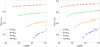 |
Fig. 1. Standard evolutionary tracks using the Vink’s recipe for mass-loss rates, with Z/Z⊙ = 1.0 (left panel) and Z/Z⊙ = 0.2 (right panel). Location of the standard stars used to create the grid of self-consistent mass-loss rates are shown by the dots. |
Names of the classical evolutionary tracks for the sets of standard stars used to calculate Ṁsc.
Given the solutions for line-force parameters employed by Gormaz-Matamala et al. (2019, 2022), we determined new self-consistent values for the mass-loss rates of these selected standard stars. These standard stars are named -01, -02, -03, and so on, as a function of the respective standard track from Table 1, and they are selected so as to keep an almost constant distance in the space of Teff and log g. The total number of standard stars varies per track, depending on the width of the range of temperatures and gravities before reaching the thresholds for the m-CAK prescription. Results are shown in Table 2 for solar metallicity (Z/Z⊙ = 1.0), in Table 3 for Z/Z⊙ = 0.5, and in Table 4 for Z/Z⊙ = 0.2. Error bars associated to the wind parameters, v∞ and Ṁsc, are based on the uncertainties of the line-force parameters as described in Gormaz-Matamala et al. (2022). Comparisons between these new self-consistent values for Ṁ and those used previously, determined by the Vink’s formula, are also included. In addition, we add an extra column comparing our Ṁsc with the theoretical values provided by Krtička & Kubát (2017, hereafter KK17, see their Eq. (11)) and Krtička & Kubát (2018, hereafter KK18, see their Eq. (1)) because their formulae are also based on a theoretical prescription for the stellar wind, although both formulae describe mass-loss rate only as a function of stellar luminosity.
4.2. Statistical fit
Given the grid of values for theoretical self-consistent mass-loss rate Ṁsc outlined in Tables 2–4, we proceed with the statistical analysis to generate an easy-to-implement formula, comparable to the known Vink’s formula. For that reason, we explore three possibilities for fitting:
– linear fitting:
 (3)
(3)
– quadratic fitting:
 (4)
(4)
– intervariable fitting:
 (5)
(5)
where Y is our fitted mass-loss rate (expressed either as Ṁ or log Ṁ), and x1, …, xN are our individual stellar parameters (temperature, gravity, radius, and metallicity). A linear fit was previously implemented by KK17 and Gormaz-Matamala et al. (2019), whereas quadratic fitting is used by Vink’s formula. Besides these options, we include the intervariable fitting in order to determine any potential inter-dependence among the individual stellar parameters.
For each of the three introduced alternatives, stellar parameters are evaluated in their linear (xi), inverse (1/xi), and logarithmical (log xi) scales, looking for the combination which best satisfies our criteria. The criteria that we use to select a good fit are as follows:
-
A value as close possible to 1 for the coefficient of determination R-squared (R2).
-
High values of t-statistic for each linear parameter.
-
As low a dispersion as possible between the real (i.e., the value from the Tables 2–4) and predicted Ṁsc, weighted by the error bars Δ Ṁ. We then define our weighted deviation as
 (6)
(6)
The advantage of adopting this weighted deviation is that we can gauge the difference between predicted and real mass-loss rates in terms relative to the intrinsic uncertainty for our results, as outlined in Gormaz-Matamala et al. (2022). Given the definition of Σw, it becomes evident that a value lower than 1 is the most idealistic result because it implies the predicted response of our fit lies below the intrinsic error of our models. This means the more reduced the spread of the deviations, the better the fit. Therefore, we expect to find a dispersion with the highest percentage of the sample below the thresholds Σw = 2 and Σw = 3.
Combining the results of the stellar wind models from Tables 2–4 with those coming from Tables 1 and 2 from Gormaz-Matamala et al. (2022), we get a total set of 116 self-consistent mass-loss rates. The results of our three fitting procedures are presented in Table 5. It is observed that all three attempts present a good prediction potential based on their R2 ≃ 1, even though the intervariable fitting presents the closest approximation to unity. This can also be seen in Fig. 2, where the three attempts closely match the ideal Ṁpredicted = Ṁreal, with the intervariable fitting slightly standing out against the other two. If we consider the normalisation by the error bars of the self-consistent mass-loss rates, and we plot histograms for the distribution of the Σw factor (see Fig. 3), we observe a smaller spread for the quadratic fitting, but the intervariable fitting keeps the highest percentage of the sample below Σw ≤ 3, with ∼90%. This is illustrated in Table 6, where both the quadratic and the intervariable fittings show a large percentage of the sample satisfying the thresholds Σw ≤ 2 and Σw ≤ 3 (over 68% and 87% respectively), with the intervariable fitting showing a slight advantage. Because this result is in agreement with the statistics found for R2, we decided to employ the intervariable fitting hereafter.
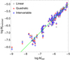 |
Fig. 2. Distribution of the obtained mass-loss rate values from our three alternatives for fitting (linear, quadratic and intervariable) in comparison with the true theoretical mass-loss rate coming from self-consistent wind solutions. |
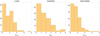 |
Fig. 3. Histograms of our weighted deviation Σw for our three attempts of fitting: linear, quadratic and intervariable. |
Coefficient of determination R2 obtained for our three alternatives for fitting.
Coefficient of determination R2 obtained for our three alternatives for fitting.
Therefore, the new formula to obtain predicted values for mass-loss rates based on the self-consistent wind solutions from Gormaz-Matamala et al. (2019, 2022) is:
 (7)
(7)
where w, x, y, and z are defined as:
Hence, this formula forms the basis of the self-consistent evolutionary tracks for the following sections of this paper. However, we include Appendix A where we introduce the parameters for the alternative linear and quadratic fittings for illustrative purposes.
One aspect that becomes clear from Eq. (7) and represents an important difference with previous studies is that this intervariable fitting does not establish a rigid relationship between the mass-loss rate and the metallicity. Instead, we formulate an interrelationship with the other stellar parameters. From Vink et al. (2001), it was determined that Ṁ ∼ Z0.69±0.10 for O-type stars; whereas Mokiem et al. (2007) determined Ṁ ∼ Z0.83±0.16 (see review from Smith 2014) and, more recently, Björklund et al. (2021) determined Ṁ ∼ Z0.95. In contrast, Vink & Sander (2021) provided a less steep relationship of Ṁ ∼ Z0.42 for O-type stars. On the contrary, from Eq. (7) and Tables 2–4, we derive that the scale between mass-loss rate and metallicity is easily correlated with the stellar mass. Therefore, for a star born with 120 M⊙, the relationship is Ṁ ∼ Z0.53±0.01 (an exponent far below the ∼0.85 found by previous authors with the exception of Vink & Sander 2021), but for stars of 25 M⊙ the relationship scales up to Ṁ ∼ Z1.02±0.05. Intermediate exponents are then found for the stars with 70 M⊙ (Ṁ ∼ Z0.61±0.02) and with 40 M⊙ (Ṁ ∼ Z0.81±0.05; which is closer to those found by previous authors). Such a deviation of the exponents for the relationship between mass-loss rate and metallicities demonstrates that this is not unique for all stars, and that stellar mass must be considered.
We then incorporate Eq. (7) as an extra option for the treatment of mass-loss rate in GENEC, for Teff ≥ 30 kK and log g ≥ 3.2. Below each of these values, the mass-loss recipe is switched to the formula from Vink et al. (2001). The effects on the evolutionary tracks of massive stars and their main implications are discussed in Sect. 5.
4.3. Variance of element abundances
The search for new line-force parameters is not limited to the variations in effective temperature, surface gravity; and stellar radius, but includes abundances. One of the great advantages of the m-CAK prescription is the ability to modify the abundances of the individual elements that compose the stellar wind. Even when metallicity can be considered as constant through the entire evolutionary track, nucleosynthesis processes throughout the evolution imply switches in the abundances for some elements. In turn, changes in the He-to-H ratio or in the individual abundances of metal elements affect the resulting line acceleration1 and therefore affect the final mass-loss rate. We also studied such effects produced by abundances in order to incorporate them into the final expressions for Ṁ. Because GENEC does not provide surface abundances for important metals such as the iron group, our analysis of individual metal elements is limited to CNO elements.
Nevertheless, from the classical evolutionary tracks tabulated in Table 1, the only one that exhibits changes on surface abundances for CNO elements and the He-to-H ratio is the track P120z10 for solar-metallicity and initial mass 120 M⊙. This is a direct consequence of working with non-rotating models: reactions in the core abruptly modify the abundance structure at some point for only extremely high-mass cases such as 120 M⊙. On the contrary, evolutionary tracks considering rotation exhibit a gradual modification of surface abundances even for stars with masses below 25 M⊙ (Ekström et al. 2012). For the low-metallicity scenarios, the non-rotating tracks show an even later break-up for the surface abundances (Georgy et al. 2013; Eggenberger et al. 2021). For this reason, our analysis of the changes in abundances affecting the self-consistent mass-loss rate is limited to the case of the track P120z10, as follows.
We extracted the stellar models from the track P120z10, specifically the models from -05 to -09, because these are the only standard stars with modifications in their abundances at the stellar surface. We then recalculated their self-consistent (k, α, δ), according to thee latter modifications in surface abundances. The results are shown in Table 7. We see that, for each of these individual models, a wind solution for the line-force parameters is in turn performed for each observed variation in the abundance and subsequently a new Ṁsc is calculated. The ratios between these new mass-loss rates (with modified individual abundances) and the Msc with default abundances are shown in Fig. 4 for the He-to-H ratio and in Fig. 5 for the CNO elements.
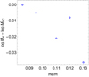 |
Fig. 4. Comparison between the resulting self-consistent mass-loss rate when the initial value for He to H ratio is modified, and the Ṁsc with the default value [He/H] = 0.085. |
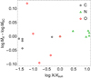 |
Fig. 5. Comparison between the resulting self-consistent mass-loss rate when the abundance for any of the CNO elements is modified, and the Ṁsc with the default solar value. |
However, these variations confirm that it is not possible to establish a clear dependence between the abundances and the mass-loss rate, especially if we consider that the error bars for the values of Ṁsc lie between ±0.06 and ±0.11. In other words, the erratic variances presented in Table 7 and in Figs. 4 and 5 can be better explained as a product of the uncertainties carried from the self-consistent wind solution instead. Given this result, we decided not to include effects from variations in the surface CNO elements or in the He-to-H ratio over the theoretical mass-loss rate. Such analyses are deferred to a forthcoming study dedicated to the case of Ṁ for rotating models.
5. Evolutionary models
Hertzsprung-Russell diagrams with the different evolutionary tracks are shown in Fig. 6. The evolution of mass-loss rates is shown in Fig. 7, and the evolution of stellar masses appears in Fig. 8. For these three figures, the evolutionary tracks cover the ZAMS to the end of the H-burning stage. In addition, for each one of these figures, we include three black dots, which correspond to (i) the ZAMS-point, (ii) the point where the self-consistent recipe for the mass-loss rate ends, and (iii) the point where we reach the end of the H-burning stage. We use these points as tracers to explore the new stellar and wind structure through the different evolutionary tracks, as explained in the following subsections. Extra properties of the tracks, such as lifetimes and final surface abundances, are summarised in Table 8. Hereafter, evolutionary tracks using ṀVink are denoted again as classical tracks2, whereas tracks using Ṁsc are referred to as self-consistent tracks.
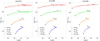 |
Fig. 6. Evolutionary tracks followed across the Hertzsprung-Russell diagram for model stars without rotation, assuming the mass-loss rates given originally from Vink et al. (2000, dashed lines, i.e., classical tracks) and those Ṁsc given by the self-consistent wind solutions from Gormaz-Matamala et al. (2022, continue lines, i.e., self-consistent tracks). Black dots represent: (i) the ZAMS-point, (ii) where Ṁsc switches to ṀVink, and (iii) the end of the H-burning stage. |
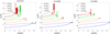 |
Fig. 7. Evolution of Ṁ of evolutionary tracks for stars with 120, 70, 40 and 25 M⊙, calculated for self-consistent tracks (solid lines) and for classical tracks (dashed lines). Black dots represent the same as indicated in Fig. 6. |
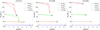 |
Fig. 8. Evolution of the stellar masses M* of our evolutionary tracks for stars with 120, 70, 40 and 25 M⊙, calculated for self-consistent tracks (solid lines) and for classical tracks (dashed lines). Black dots represent the same as indicated in Fig. 6. |
Properties of the stellar models at the end of the H-burning phases.
The most remarkable result from Fig. 6 is that self-consistent evolutionary tracks drift towards more luminous scales in the HRDs. Such movements seem to be a direct consequence of Ṁsc being less strong than ṀVink, as shown in Fig. 7. Stars evolving within self-consistent tracks retain more mass than within classical tracks (Fig. 8), resulting in both more massive and larger stars in terms of stellar radii (Fig. 9) and more luminous stars in turn. The direct relation between the mass and the radius of the stars becomes more evident if we plot the so-called spectroscopic HRD (sHRD, Langer & Kudritzki 2014), where we observe that there is no significant difference between the surface gravities – which are proportional to  – from the different tracks (Fig. 10).
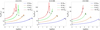 |
Fig. 9. Evolution of the stellar radii R* of our evolutionary tracks for stars with 120, 70, 40 and 25 M⊙, calculated for self-consistent tracks (solid lines) and for classical tracks (dashed lines). Black dots represent the same as indicated in Fig. 6. |
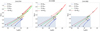 |
Fig. 10. Evolutionary tracks across the spectroscopic Hertzsprung-Russell diagram (Langer & Kudritzki 2014) for model stars without rotation, calculated for self-consistent tracks (solid lines) and for classical tracks (dashed lines). Grey shaded area represents the region where self-consistent m-CAK prescription is valid (Teff ≥ 30, log g ≥ 3.2, see Gormaz-Matamala et al. 2022). Black dots represent the same as indicated in Fig. 6. |
This departure between the projected tracks is more prominent for higher masses and metallicities; which can be attributed to the greater difference in mass-loss rate between self-consistent and Vink’s formula for these cases, but also to the absolute quantity of the mass-loss rate, as seen in Fig. 7. Moreover, this is also in agreement with the level of relevance that mass loss has for the evolution of O-type stars: from full dominance for stars with M ≳ 60 M⊙ (Vink & Gräfener 2012); a slightly less relevant role for stars with 30 M⊙ < M* < 60M⊙ (Langer 2012; Groh et al. 2014); and a secondary influence for stars with M* < 30M⊙, where features such as rotation (absent in our study) appear to dominate (Maeder & Meynet 2000).
5.1. Cases where MZAMS = 120 M⊙
As expected, the largest differences between the evolutionary tracks using our self-consistent prescription for mass-loss rate are given for the most massive cases. This is particularly evident from Fig. 8, where the differences in the evolution of the stellar masses are more pronounced, especially for the more metallic cases. Stars from the tracks using Ṁsc lose their masses at a slower rate, retaining ∼20 M⊙ of extra mass for the Galactic case (Z = 0.014), ∼10 M⊙ for the Large Magellanic Cloud (LMC, Z = 0.006) case, and ∼5 M⊙ for the Small Magellanic Cloud case (SMC, Z = 0.002) compared with the standard tracks at the end of the model calculation with the self-consistent recipe (second dot in the plots). These differences in mass decrease later, where we observe that the Galactic case suffers a sudden loss of mass (seen also in the eruptive increment in Ṁ from Fig. 7) before the end of the hydrogen-burning stage and then finishes with a stellar mass that is greater by only ∼4 − 5 M⊙ than the classical track (see Table 8). A similar sudden loss of mass is also seen in the LMC case, making the final M* at the end of the H-burning stage almost the same as for the classical track. These ‘eruptive processes’ are a consequence of the switch in mass-loss rate due to the bi-stability jump around Teff ∼ 25 kK (Vink et al. 1999) according to the Vink’s formula. Vink et al. (1999) suggested that such an increase might be related to typical variations shown by luminous blue variable (LBV) stars. In addition, Groh et al. (2014) demonstrated that stars born with more than 60 M* reach the LBV spectroscopic phase before the end of the H-core-burning stage. However, recently, new wind models shed doubt on the reality of this wind enhancement (Björklund et al. 2022).
The Galactic case presents similar stellar radii for both classical and self-consistent tracks at the end of the H-burning stage, despite the fact that the radii for the self-consistent track present an extra peak around ∼2 Myr which coincides with the eruptive increase in mass-loss rate. This extra peak is also observed for the self-consistent track for the LMC, although here the final radius is reduced by ∼26% with respect to that seen with the classical track. However, the most remarkable difference in stellar radius comes from the SMC case, which generates the largest stellar sizes at the end of the H-core-burning stage (see Table 8) and where the final R* for the self-consistent track is ∼30% of that of the classical track. This can be attributed to the eruptive increment in mass-loss rate due to eruptions being less abrupt than in the more metallic cases (indeed, this is around one order of magnitude smaller for SMC, as shown in Fig. 7) and therefore the increase in stellar radius is not interrupted. This hypothesis is reinforced if we take into account the fact that the LBV stage is not thought to be independent of the mentioned bi-stability jump (Vink et al. 1999), which is produced when iron recombines from Fe IV to Fe III. Naturally, the contribution of Fe lines to the line acceleration in tracks with metallicity Z = 0.002 is less relevant than in the other cases and therefore the switch in mass-loss rate is smaller.
In summary, eruptive processes associated to the LBV stage affect stellar evolution for high-metallicity objects (of the Galaxy and LMC) with different consequences. At solar metallicity, stellar radius is almost the same (for classical and self-consistent tracks) and a difference is seen in the final mass at the end of the H-burning stage. On the contrary, final masses are quite similar for the LMC metallicity but the self-consistent track generates a much smaller star at the end of the H-burning stage. According to what is observed for the models with MZAMS = 70 M⊙ (see following subsection), we certify that the case of similar radii and different final masses is exceptional, and can therefore be attributed to the peculiar conditions of MZAMS = 120 M⊙ at solar metallicity. After all, this is the track with the most extreme mass-loss rates and the only one with remarkable modifications in its surface abundances.
Moreover, these initial cases with MZAMS = 120 M⊙ are the only instances where the surface abundances undergo significant modification at the end of the H-burning stage for all the metallicities (last three columns of Table 8). Self-consistent tracks present slightly more helium at their surfaces at the end of the H-burning stages, particularly for Galactic and LMC cases, even when timescales are marginally shorter. We interpret these differences as a consequence of the bigger convective core as shown in Fig. 11 and of the mass losses. Changes in the chemical composition are directly linked with the decrease in mass of the convective core. Depending on the mass-loss rate, layers having belonged to those regions partly processed by H-burning are exposed to the surface. The value of He enrichment obtained at the surface is therefore the product of interplay between mass loss and convective core evolution.
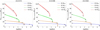 |
Fig. 11. Evolution of the mass of the convective-core Mcc (relative to the total stellar mass M*), of our evolutionary tracks for stars with 120, 70, 40 and 25 M⊙, calculated using our self-consistent Ṁsc (solid lines) and using Vink’s formula ṀVink (dashed lines). Black dots represent the same as indicated in Fig. 6. |
5.2. Cases where MZAMS = 70 M⊙
Here we observe a similar trend to the former MZAMS = 120 M⊙ case, but on a smaller scale. Tracks using Ṁsc retain ∼15 M⊙ of extra mass for the Galactic case this time, ∼10 M⊙ for the LMC case, and ∼3 M⊙ for the SMC case at the end of the self-consistent recipe. Again, eruptive increments in mass-loss rate after the end of the stage using Ṁsc compensate these initial differences in the evolution of the stellar masses, and once more we obtain similar M* at the end of the H-burning stage. However, now we observe for all our metallicities that self-consistent tracks predict smaller stellar radii, although the biggest differences are given for Galactic and LMC cases.
Another similarity with the MZAMS = 120 M⊙ case is that we observe an extra peak for the stellar radii when solar metallicity is adopted, coinciding with the eruptive increment in Ṁ. Hence, we could argue that the higher retention of mass for the self-consistent tracks produces larger stars that reach closer to the Eddington limit and then generate larger eruptions in the LBV stage.
5.3. Cases where MZAMS = 40 M⊙ and MZAMS = 25 M⊙
For these two initial masses, the differences between classical and self-consistent tracks are only marginal, with the expected increase in luminosity for the HRDs (Fig. 6) and slightly larger stellar radii and masses at the end of H-burning stage (Table 8) even after shorter timescales. However, despite these differences being minor, they reinforce the significant trend that is observed: because Ṁsc < ṀVink, self-consistent tracks produce larger and brighter stars, reaching the end of the H-burning stage on a shorter timescale.
One particular model that merits attention is the tracks with MZAMS = 25 and 40 M⊙ and Z = 0.002, which reach the end of the H-burning stage without leaving the range of validity for Msc and therefore present only two black dots. We can observe such peculiarity in Fig. 10, where the track remains limited to the region Teff ≥ 32 kK and log g ≥ 3.2. This is interesting because it means that the m-CAK self-consistent prescription is able to describe the wind hydrodynamics for massive stars at He-burning stages, when masses are ∼40 M⊙ and smaller, and metallicities are very low. We will explore this matter further in a forthcoming study, where we will explore self-consistent solutions for stages with burning processes beyond hydrogen.
6. Some consequences of the new hydrodynamic wind model
The consequences of the new hydrodynamic wind models remain modest for many outputs of the stellar models, such as the evolutionary tracks in the HRD (Fig. 6) or the evolution of the convective cores (Fig. 11). On the other hand, for the most massive stars at solar metallicity, the impact on the evolution of the total mass as a function of time is significant (see the left panel of Fig. 8 and especially at 120 M⊙). Therefore, in this metallicity and mass domain, the adoption of the new hydrodynamic wind models may indeed have a significant impact on some model outputs.
One obvious consequence is the impact on the wind enrichment of the interstellar medium in isotopes produced in massive stars during the core-hydrogen-burning phase. The radionuclide isotope 26Al is a good example. It is produced by proton capture on 25Mg in the convective cores of stars with masses above about 25 M⊙ (see Prantzos & Casse 1986; Meynet et al. 1997; Palacios et al. 2005) and can be ejected by stellar winds. Figure 12 shows how the mass fraction of 26Al evolves as a function of time at the centre and at the surface of two 120 M⊙ models at solar metallicity computed with the Vink’s formula (top panel) and with the new hydrodynamic wind model (bottom panel). We see that in the model computed with the new mass-loss rates, slightly higher (around ∼10% more) central abundances are reached for 26Al. This is due to the fact that the actual mass remains larger because the mass-loss rates are decreased. This allows the convective core to be slightly larger (see the left panel of Fig. 11), therefore increasing the central temperature and thus allowing larger abundances of 26Al to be reached (the peak abundance is reached when the production rate by proton capture on 25Mg is balanced by the decay rate; if the temperatures are higher, the proton capture rate is higher and greater abundances are reached). However, obtaining greater abundances at the centre does not necessarily imply that more 26Al is ejected by stellar winds. Indeed, lower winds imply that the layers that once belonged to the core and that have become enriched in 26Al appear at later stages, when enough time has elapsed for the 26Al abundance to decay in those layers exposed at the surface. This, despite the production of 26Al in the core, is the same when we adopt Ṁsc instead of Vink’s formula. One consequence is the decrease in the wind contribution of in 26Al from massive stars integrated throughout their lifetime. Let us reiterate here that thanks to the observed diffuse emission at 1.8 MeV produced by the decay of 26Al present in the Galactic interstellar medium, we know that presently our Galaxy contains a quantity of 26Al of between 1.7 and 3.5 M⊙ (Knödlseder 1999; Diehl et al. 2006; Wang et al. 2009). The winds of massive stars might contribute about 1 M⊙, which is about half or one-third of the total content in this isotope of the Milky Way (see e.g. Palacios et al. 2005). The new mass-loss rates would decrease this contribution by about a factor two, which can be easily seen if we integrate the mass fraction of 26Al on the surface over the lifetime of the stellar model (see Table 9). However, a more detailed study is required to properly quantify the consequences of the new mass-loss rates for the entire lifetime of massive stars including phases such as the WR one. Nevertheless, it is clear that the wind contribution from single stars will be decreased, leaving more room for the supernova contribution and binary systems.
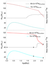 |
Fig. 12. Evolution as a function of time of the total mass (red curve), of the mass fraction of 26Al at the centre and at the surface of 120 M⊙ at Z = 0.014. Top panel: the case when the Vink’s formula for the mass-loss rate is adopted. Bottom panel: the case when the new rates obtained from hydrodynamic wind models are used. Note that making the plot more easily readable the curves for the mass fraction have been obtained by multiplying the mass fraction by a constant factor and the starting point of each curves has been shifted upwards along the Y axis (see the figure for the adopted values). Black dots represent the same as indicated in Fig. 6. |
Further significant consequences of these lower mass-loss rates may be seen when considering the evolution of massive stars with a surface magnetic field. Only 8%–10% of the OB stars have a surface magnetic field that can be measured (Wade & Neiner 2018). For those massive magnetic stars, the surface magnetic field can have important effects, slowing down the star through the process of wind magnetic braking (Meynet et al. 2011; Keszthelyi et al. 2021) or by decreasing the mass that is lost by stellar winds through the process of wind magnetic quenching (Owocki et al. 2016; Petit et al. 2017; Georgy et al. 2017). The importance of these processes depends on how the density of kinetic energy in the wind (which depends on the mass-loss rates) compares to the density of magnetic energy. Decreasing the mass-loss rates, with everything else kept constant, increases the impact of the magnetic field on the evolution of massive stars. As indicated above, dedicated models need be made in order to quantity the impact of the new mass-loss rates considered here on these magnetic effects. We suspect that the effects are significant.
7. Summary and conclusions
We implemented our new mass-loss rates, Ṁsc, in GENEC and computed the evolution of massive stars with different initial masses and metallicities with this new prescription. Mass-loss rates used for this study are based on the self-consistent m-CAK prescription for wind solutions performed by Gormaz-Matamala et al. (2019, 2022), replacing the classical Vink’s formula (Vink et al. 2000, 2001) with our new formula.
To achieve this, we developed a recipe for Ṁsc,predicted (Eq. (7)) and performed a statistical analysis, establishing that the ‘intervariable fit’ (with stellar parameters combined with each other) leads to a more reduced deviation between the predicted and real, self-consistent mass-loss rates. This intervariable fit also allows us to explore the Ṁ ∝ Za relationship. We find that the exponent a depends on the stellar mass: the more massive the star, the smaller the a exponent. This may be due to the fact that the more massive the star, the nearer it is from the Eddington limit. In that case, the continuum may become increasingly important in contributing to the winds. The effect of continuum is less dependant on metallicity because it is does not involve interaction between the radiative field and absorption lines.
Because global values for mass-loss rates provided by the m-CAK prescription are lower than the values provided by the Vink’s formula, self-consistent tracks retain more mass during their evolution. As a consequence, they produce larger and more luminous stars, as can be seen in the HRDs (Fig. 6). Such differences are more prominent for our models with higher initial masses, confirming that mass-loss rate plays a more relevant role throughout stellar evolution for very massive stars on the order of M* ≳ 60 M⊙ (Vink & Gräfener 2012). These larger radii for the self-consistent tracks also cause the evolution model to approach closer to the Eddington limit and then to experience the eruptive increases in mass-loss rate associated with the LBV stage prior to the end of the H-burning stage (Groh et al. 2014). In addition, we observe that the most massive stars present slightly shorter lifetimes and end their H-burning stage with a larger percentage of helium abundance on their surface.
Nevertheless, the most remarkable difference between classic and self-consistent tracks is the generation and abundance of 26Al on the stellar surface of our model with M* = 120 M⊙ and Z = 0.014, which suggest that the contribution of this isotope from stellar winds to the Galactic interstellar medium is less than previously thought.
These promising results highlight the necessity to extend this current study to a wider range of evolutionary stages, to include rotation, and to constrain the populations of massive stars in the Galaxy and beyond. Because self-consistent tracks are based on smaller mass-loss rates (and subsequently more massive and larger stars), we could speculate that the loss of angular momentum should be lower. Such extra elements, and their consequences, will be included in a forthcoming paper.
GENEC provides the changes in abundances both at the core of the star and at its surface. However, for the calculation of line acceleration we are interested only in the modification of abundances at the surface of the star.
Acknowledgments
This project has received funding from the European Unions Framework Programme for Research and Innovation Horizon 2020 (2014-2020) under the Marie Skłodowska-Curie grant Agreement NO 823734. A.C.G.M. has been financially supported by the PhD Scholarship folio NO 21161426 from National Commission for Scientific and Technological Research of Chile (CONICYT). A.C.G.M. and M.C. acknowledge support from Centro de Astrofísica de Valparaíso. M.C. thanks the support from FONDECYT project 1190485. J.C. thanks the support from FONDECYT project 1211429. A.C.G.M. and J.C. are grateful of the support from Max Planck Partner Group on Galactic Centre Astrophysics. G.M. has received funding from the European Research Council (ERC) under the European Union’s Horizon 2020 research and innovation programme (grant agreement No 833925, project STAREX). J.H.G. and L.M. wish to acknowledge the Irish Research Council for funding this research.
References
- Abbott, D. C. 1982, ApJ, 259, 282 [Google Scholar]
- Araya, I., Jones, C. E., Curé, M., et al. 2017, ApJ, 846, 2 [NASA ADS] [CrossRef] [Google Scholar]
- Asplund, M., Grevesse, N., & Sauval, A. J. 2005, in osmic Abundances as Records of Stellar Evolution and Nucleosynthesis, eds. I. Barnes, G. Thomas, & F. N. Bash, ASP Conf. Ser., 336, 25 [NASA ADS] [Google Scholar]
- Asplund, M., Grevesse, N., Sauval, A. J., & Scott, P. 2009, ARA&A, 47, 481 [NASA ADS] [CrossRef] [Google Scholar]
- Björklund, R., Sundqvist, J. O., Puls, J., & Najarro, F. 2021, A&A, 648, A36 [EDP Sciences] [Google Scholar]
- Björklund, R., Sundqvist, J. O., Singh, S. M., Puls, J., & Najarro, F. 2022, A&A, 648, A36 [Google Scholar]
- Bouret, J. C., Lanz, T., & Hillier, D. J. 2005, A&A, 438, 301 [NASA ADS] [CrossRef] [EDP Sciences] [Google Scholar]
- Bouret, J. C., Hillier, D. J., Lanz, T., & Fullerton, A. W. 2012, A&A, 544, A67 [NASA ADS] [CrossRef] [EDP Sciences] [Google Scholar]
- Brott, I., de Mink, S. E., Cantiello, M., et al. 2011, A&A, 530, A115 [NASA ADS] [CrossRef] [EDP Sciences] [Google Scholar]
- Castor, J. I., Abbott, D. C., & Klein, R. I. 1975, ApJ, 195, 157 [Google Scholar]
- Curé, M. 2004, ApJ, 614, 929 [CrossRef] [Google Scholar]
- Diehl, R., Halloin, H., Kretschmer, K., et al. 2006, Nature, 439, 45 [CrossRef] [PubMed] [Google Scholar]
- Eggenberger, P., Meynet, G., Maeder, A., et al. 2008, Ap&SS, 316, 43 [Google Scholar]
- Eggenberger, P., Ekström, S., Georgy, C., et al. 2021, A&A, 652, A137 [NASA ADS] [CrossRef] [EDP Sciences] [Google Scholar]
- Ekström, S., Georgy, C., Eggenberger, P., et al. 2012, A&A, 537, A146 [Google Scholar]
- Georgy, C., Ekström, S., Eggenberger, P., et al. 2013, A&A, 558, A103 [NASA ADS] [CrossRef] [EDP Sciences] [Google Scholar]
- Georgy, C., Meynet, G., Ekström, S., et al. 2017, A&A, 599, L5 [NASA ADS] [CrossRef] [EDP Sciences] [Google Scholar]
- Gormaz-Matamala, A. C., Curé, M., Cidale, L. S., & Venero, R. O. J. 2019, ApJ, 873, 131 [NASA ADS] [CrossRef] [Google Scholar]
- Gormaz-Matamala, A. C., Curé, M., Hillier, D. J., et al. 2021, ApJ, 920, 64 [NASA ADS] [CrossRef] [Google Scholar]
- Gormaz-Matamala, A. C., Curé, M., Lobel, A., et al. 2022, A&A, 661, A51 [NASA ADS] [CrossRef] [EDP Sciences] [Google Scholar]
- Gräfener, G., Koesterke, L., & Hamann, W.-R. 2002, A&A, 387, 244 [NASA ADS] [CrossRef] [EDP Sciences] [Google Scholar]
- Groh, J. H., Meynet, G., Ekström, S., & Georgy, C. 2014, A&A, 564, A30 [NASA ADS] [CrossRef] [EDP Sciences] [Google Scholar]
- Groh, J. H., Ekström, S., Georgy, C., et al. 2019, A&A, 627, A24 [NASA ADS] [CrossRef] [EDP Sciences] [Google Scholar]
- Hamann, W.-R., & Gräfener, G. 2003, A&A, 410, 993 [CrossRef] [EDP Sciences] [Google Scholar]
- Heger, A., Fryer, C. L., Woosley, S. E., Langer, N., & Hartmann, D. H. 2003, ApJ, 591, 288 [CrossRef] [Google Scholar]
- Hillier, D. J. 1990a, A&A, 231, 111 [NASA ADS] [Google Scholar]
- Hillier, D. J. 1990b, A&A, 231, 116 [NASA ADS] [Google Scholar]
- Hillier, D. J., & Miller, D. L. 1998, ApJ, 496, 407 [NASA ADS] [CrossRef] [Google Scholar]
- Iglesias, C. A., & Rogers, F. J. 1996, ApJ, 464, 943 [NASA ADS] [CrossRef] [Google Scholar]
- Keszthelyi, Z., Meynet, G., Martins, F., de Koter, A., & David-Uraz, A. 2021, MNRAS, 504, 2474 [NASA ADS] [CrossRef] [Google Scholar]
- Knödlseder, J. 1999, ApJ, 510, 915 [CrossRef] [Google Scholar]
- Krtička, J., & Kubát, J. 2017, A&A, 606, A31 [NASA ADS] [CrossRef] [EDP Sciences] [Google Scholar]
- Krtička, J., & Kubát, J. 2018, A&A, 612, A20 [NASA ADS] [CrossRef] [EDP Sciences] [Google Scholar]
- Langer, N. 2012, ARA&A, 50, 107 [CrossRef] [Google Scholar]
- Langer, N., & Kudritzki, R. P. 2014, A&A, 564, A52 [NASA ADS] [CrossRef] [EDP Sciences] [Google Scholar]
- Maeder, A. 1983, A&A, 120, 113 [NASA ADS] [Google Scholar]
- Maeder, A. 1987, A&A, 173, 247 [NASA ADS] [Google Scholar]
- Maeder, A., & Meynet, G. 1987, A&A, 182, 243 [NASA ADS] [Google Scholar]
- Maeder, A., & Meynet, G. 2000, A&A, 361, 159 [NASA ADS] [Google Scholar]
- Meynet, G., Maeder, A., Schaller, G., Schaerer, D., & Charbonnel, C. 1994, A&AS, 103, 97 [Google Scholar]
- Meynet, G., Arnould, M., Prantzos, N., & Paulus, G. 1997, A&A, 320, 460 [NASA ADS] [Google Scholar]
- Meynet, G., Eggenberger, P., & Maeder, A. 2011, A&A, 525, L11 [CrossRef] [EDP Sciences] [Google Scholar]
- Meynet, G., Chomienne, V., Ekström, S., et al. 2015, A&A, 575, A60 [NASA ADS] [CrossRef] [EDP Sciences] [Google Scholar]
- Meynet, G., Eggenberger, P., Mowlavi, N., & Maeder, A. 2009, in The Ages of Stars, eds. E. E. Mamajek, D. R. Soderblom, & R. F. G. Wyse, 258, 177 [NASA ADS] [Google Scholar]
- Mokiem, M. R., de Koter, A., Vink, J. S., et al. 2007, A&A, 473, 603 [NASA ADS] [CrossRef] [EDP Sciences] [Google Scholar]
- Muijres, L., Vink, J. S., de Koter, A., et al. 2012, A&A, 546, A42 [NASA ADS] [CrossRef] [EDP Sciences] [Google Scholar]
- Owocki, S. P., ud-Doula, A., Sundqvist, J. O., et al. 2016, MNRAS, 462, 3830 [NASA ADS] [CrossRef] [Google Scholar]
- Palacios, A., Meynet, G., Vuissoz, C., et al. 2005, A&A, 429, 613 [NASA ADS] [CrossRef] [EDP Sciences] [Google Scholar]
- Pauldrach, A., Puls, J., & Kudritzki, R. P. 1986, A&A, 164, 86 [NASA ADS] [Google Scholar]
- Petit, V., Keszthelyi, Z., MacInnis, R., et al. 2017, MNRAS, 466, 1052 [NASA ADS] [CrossRef] [Google Scholar]
- Prantzos, N., & Casse, M. 1986, ApJ, 307, 324 [NASA ADS] [CrossRef] [Google Scholar]
- Puls, J., Urbaneja, M. A., Venero, R., et al. 2005, A&A, 435, 669 [NASA ADS] [CrossRef] [EDP Sciences] [Google Scholar]
- Puls, J., Vink, J. S., & Najarro, F. 2008, A&ARv., 16, 209 [NASA ADS] [CrossRef] [Google Scholar]
- Sander, A. A. C., Hamann, W.-R., Todt, H., Hainich, R., & Shenar, T. 2017, A&A, 603, A86 [NASA ADS] [CrossRef] [EDP Sciences] [Google Scholar]
- Santolaya-Rey, A. E., Puls, J., & Herrero, A. 1997, A&A, 323, 488 [NASA ADS] [Google Scholar]
- Smith, N. 2014, ARA&A, 52, 487 [NASA ADS] [CrossRef] [Google Scholar]
- Sundqvist, J. O., & Puls, J. 2018, A&A, 619, A59 [NASA ADS] [CrossRef] [EDP Sciences] [Google Scholar]
- Sundqvist, J. O., Björklund, R., Puls, J., & Najarro, F. 2019, A&A, 632, A126 [NASA ADS] [CrossRef] [EDP Sciences] [Google Scholar]
- Vink, J. S. 2021, ARA&A, 60, 1 [Google Scholar]
- Vink, J. S., & Gräfener, G. 2012, ApJ, 751, L34 [Google Scholar]
- Vink, J. S., & Sander, A. A. C. 2021, MNRAS, 504, 2051 [NASA ADS] [CrossRef] [Google Scholar]
- Vink, J. S., de Koter, A., & Lamers, H. J. G. L. M. 1999, A&A, 350, 181 [Google Scholar]
- Vink, J. S., de Koter, A., & Lamers, H. J. G. L. M. 2000, A&A, 362, 295 [Google Scholar]
- Vink, J. S., de Koter, A., & Lamers, H. J. G. L. M. 2001, A&A, 369, 574 [NASA ADS] [CrossRef] [EDP Sciences] [Google Scholar]
- Šurlan, B., Hamann, W. R., Kubát, J., Oskinova, L. M., & Feldmeier, A. 2012, A&A, 541, A37 [NASA ADS] [CrossRef] [EDP Sciences] [Google Scholar]
- Šurlan, B., Hamann, W. R., Aret, A., et al. 2013, A&A, 559, A130 [NASA ADS] [CrossRef] [EDP Sciences] [Google Scholar]
- Wade, G. A., & Neiner, C. 2018, Contrib. Astron. Obs. Skalnate Pleso, 48, 106 [NASA ADS] [Google Scholar]
- Wang, W., Lang, M. G., Diehl, R., et al. 2009, A&A, 496, 713 [NASA ADS] [CrossRef] [EDP Sciences] [Google Scholar]
Appendix A: Alternative fits for Ṁsc,predicted
From Section 4.2, our analysis determined that the most optimal fit to reduce discrepancies between the predicted Ṁ from a recipe and the real values for Ṁ from our grid of self-consistent solutions (Tables 2, 3 and 4) is the intervariable fitting. Nevertheless, we decide to show in this Appendix the alternative parameters for the best linear and quadratic fittings, whose coefficient of determination R2 is tabulated in Table 5.
A.1. Linear fit
 (A.1)
(A.1)
where w, x, y and z are defined as:

A.2. Quadratic fit
 (A.2)
(A.2)
where w, x, y and z are defined as:

All Tables
Names of the classical evolutionary tracks for the sets of standard stars used to calculate Ṁsc.
Coefficient of determination R2 obtained for our three alternatives for fitting.
Coefficient of determination R2 obtained for our three alternatives for fitting.
All Figures
|
Fig. 1. Standard evolutionary tracks using the Vink’s recipe for mass-loss rates, with Z/Z⊙ = 1.0 (left panel) and Z/Z⊙ = 0.2 (right panel). Location of the standard stars used to create the grid of self-consistent mass-loss rates are shown by the dots. |
| In the text | |
|
Fig. 2. Distribution of the obtained mass-loss rate values from our three alternatives for fitting (linear, quadratic and intervariable) in comparison with the true theoretical mass-loss rate coming from self-consistent wind solutions. |
| In the text | |
|
Fig. 3. Histograms of our weighted deviation Σw for our three attempts of fitting: linear, quadratic and intervariable. |
| In the text | |
|
Fig. 4. Comparison between the resulting self-consistent mass-loss rate when the initial value for He to H ratio is modified, and the Ṁsc with the default value [He/H] = 0.085. |
| In the text | |
|
Fig. 5. Comparison between the resulting self-consistent mass-loss rate when the abundance for any of the CNO elements is modified, and the Ṁsc with the default solar value. |
| In the text | |
|
Fig. 6. Evolutionary tracks followed across the Hertzsprung-Russell diagram for model stars without rotation, assuming the mass-loss rates given originally from Vink et al. (2000, dashed lines, i.e., classical tracks) and those Ṁsc given by the self-consistent wind solutions from Gormaz-Matamala et al. (2022, continue lines, i.e., self-consistent tracks). Black dots represent: (i) the ZAMS-point, (ii) where Ṁsc switches to ṀVink, and (iii) the end of the H-burning stage. |
| In the text | |
|
Fig. 7. Evolution of Ṁ of evolutionary tracks for stars with 120, 70, 40 and 25 M⊙, calculated for self-consistent tracks (solid lines) and for classical tracks (dashed lines). Black dots represent the same as indicated in Fig. 6. |
| In the text | |
|
Fig. 8. Evolution of the stellar masses M* of our evolutionary tracks for stars with 120, 70, 40 and 25 M⊙, calculated for self-consistent tracks (solid lines) and for classical tracks (dashed lines). Black dots represent the same as indicated in Fig. 6. |
| In the text | |
|
Fig. 9. Evolution of the stellar radii R* of our evolutionary tracks for stars with 120, 70, 40 and 25 M⊙, calculated for self-consistent tracks (solid lines) and for classical tracks (dashed lines). Black dots represent the same as indicated in Fig. 6. |
| In the text | |
|
Fig. 10. Evolutionary tracks across the spectroscopic Hertzsprung-Russell diagram (Langer & Kudritzki 2014) for model stars without rotation, calculated for self-consistent tracks (solid lines) and for classical tracks (dashed lines). Grey shaded area represents the region where self-consistent m-CAK prescription is valid (Teff ≥ 30, log g ≥ 3.2, see Gormaz-Matamala et al. 2022). Black dots represent the same as indicated in Fig. 6. |
| In the text | |
|
Fig. 11. Evolution of the mass of the convective-core Mcc (relative to the total stellar mass M*), of our evolutionary tracks for stars with 120, 70, 40 and 25 M⊙, calculated using our self-consistent Ṁsc (solid lines) and using Vink’s formula ṀVink (dashed lines). Black dots represent the same as indicated in Fig. 6. |
| In the text | |
|
Fig. 12. Evolution as a function of time of the total mass (red curve), of the mass fraction of 26Al at the centre and at the surface of 120 M⊙ at Z = 0.014. Top panel: the case when the Vink’s formula for the mass-loss rate is adopted. Bottom panel: the case when the new rates obtained from hydrodynamic wind models are used. Note that making the plot more easily readable the curves for the mass fraction have been obtained by multiplying the mass fraction by a constant factor and the starting point of each curves has been shifted upwards along the Y axis (see the figure for the adopted values). Black dots represent the same as indicated in Fig. 6. |
| In the text | |
Current usage metrics show cumulative count of Article Views (full-text article views including HTML views, PDF and ePub downloads, according to the available data) and Abstracts Views on Vision4Press platform.
Data correspond to usage on the plateform after 2015. The current usage metrics is available 48-96 hours after online publication and is updated daily on week days.
Initial download of the metrics may take a while.