| Issue |
A&A
Volume 667, November 2022
|
|
|---|---|---|
| Article Number | A74 | |
| Number of page(s) | 28 | |
| Section | Stellar structure and evolution | |
| DOI | https://doi.org/10.1051/0004-6361/202243670 | |
| Published online | 09 November 2022 | |
Distance estimates for AGB stars from parallax measurements⋆
1
Theoretical Astrophysics, Division for Astronomy and Space Physics, Department of Physics and Astronomy, Uppsala University, Box 516, 751 20 Uppsala, Sweden
e-mail: miora.andriantsaralaza@physics.uu.se
2
Department of Space, Earth and Environment, Chalmers University of Technology, Onsala Space Observatory, 439 92 Onsala, Sweden
Received:
29
March
2022
Accepted:
24
August
2022
Context. Estimating the distances to asymptotic giant branch (AGB) stars using optical measurements of their parallaxes is not straightforward because of the large uncertainties introduced by their dusty envelopes, their large angular sizes, and their surface brightness variability.
Aims. This paper aims to assess the reliability of the distances derived with Gaia DR3 parallaxes for AGB stars, and provide a new distance catalogue for a sample of ∼200 nearby AGB stars.
Methods. We compared the parallaxes from Gaia DR3 with parallaxes measured with maser observations with very long baseline interferometry (VLBI) to determine a statistical correction factor for the DR3 parallaxes using a sub-sample of 33 maser-emitting oxygen-rich nearby AGB stars. We then calculated the distances of a total of ∼200 AGB stars in the DEATHSTAR project using a Bayesian statistical approach on the corrected DR3 parallaxes and a prior based on the previously determined Galactic distribution of AGB stars. We performed radiative transfer modelling of the stellar and dust emission to determine the luminosity of the sources in the VLBI sub-sample based on the distances derived from maser parallaxes, and derived a new bolometric period-luminosity relation for Galactic oxygen-rich Mira variables.
Results. We find that the errors on the Gaia DR3 parallaxes given in the Gaia DR3 catalogue are underestimated by a factor of 5.44 for the brightest sources (G < 8 mag). Fainter sources (8 ≤ G < 12) require a lower parallax error inflation factor of 2.74. We obtain a Gaia DR3 parallax zero-point offset of −0.077 mas for bright AGB stars. The offset becomes more negative for fainter AGB stars. After correcting the DR3 parallaxes, we find that the derived distances are associated with significant, asymmetrical errors for more than 40% of the sources in our sample. We obtain a PL relation of the form Mbol = (− 3.31 ± 0.24) [log P − 2.5]+(−4.317 ± 0.060) for the oxygen-rich Mira variables in the Milky Way. A new distance catalogue based on these results is provided for the sources in the DEATHSTAR sample.
Conclusions. The corrected Gaia DR3 parallaxes can be used to estimate distances for AGB stars using the AGB prior, but we confirm that one needs to be careful when the uncertainties on parallax measurements are larger than 20%, which can result in model-dependent distances and source-dependent offsets. We find that a RUWE (re-normalised unit weight error) below 1.4 does not guarantee reliable distance estimates and we advise against the use of only the RUWE to measure the quality of Gaia DR3 astrometric data for individual AGB stars.
Key words: stars: AGB and post-AGB / stars: distances / parallaxes / methods: statistical
Table C.1 is also available at the CDS via anonymous ftp to cdsarc.cds.unistra.fr (130.79.128.5) or via https://cdsarc.cds.unistra.fr/viz-bin/cat/J/A+A/667/A74
© M. Andriantsaralaza et al. 2022
 Open Access article, published by EDP Sciences, under the terms of the Creative Commons Attribution License (https://creativecommons.org/licenses/by/4.0), which permits unrestricted use, distribution, and reproduction in any medium, provided the original work is properly cited.
This article is published in open access under the Subscribe-to-Open model. Subscribe to A&A to support open access publication.
1. Introduction
Distance is one of the most fundamental parameters in astronomy which lies at the basis of the analysis and interpretation of astronomical data. The Gaia mission (Gaia Collaboration 2016a) aims to provide accurate measurements of the position, the parallax, and the proper motions of about 1% of the stars in the Milky Way with accuracies 100 times better than its predecessor HIPPARCOS. Its astrometric instrument covers wavelengths between 330 and 1050 nm, defining the photometric G band (Carrasco et al. 2016; Gaia Collaboration 2016a,b; van Leeuwen et al. 2017). The third Gaia data release (DR3), recently published by Gaia Collaboration (2022), corresponds to an observing time of 34 months. The corresponding astrometry was published in an early third data release (Gaia Collaboration 2021, hereafter eDR3), with nominal parallax uncertainties of 0.02 − 0.03 mas for G < 15, 0.07 mas at G = 17, 0.5 mas at G = 20, and 1.3 mas at G = 21 mag. We note that the values of all the parameters relevant to this work (e.g. parallax, parallax error, G magnitude) are identical in the Gaia eDR3 and DR3 catalogues for the sources discussed in this paper.
Determining the distances to asymptotic giant branch (AGB) stars using parallaxes measured with optical telescopes such as Gaia is, however, not a simple task. Comparative studies such as the analysis by Xu et al. (2019) based on Gaia data release 2 (DR2; Gaia Collaboration 2018) show that the precision of the Gaia parallaxes depends on the colour of the star: the redder the star, the larger the errors. This is because red stars are usually larger, show more surface brightness variation, and have more dust. This is true for AGB stars. The AGB phase is the evolutionary stage at which low-to-intermediate-mass stars lose mass through slow and massive stellar winds, with mass-loss rates reaching up to 10−4 M⊙ yr−1 (Höfner & Olofsson 2018). The material ejected from the star forms a large envelope mainly consisting of molecules and dust, called the circumstellar envelope (CSE). Therefore, interstellar and circumstellar dust both contribute to making AGB stars nearly invisible in the optical range of the electromagnetic spectrum. In addition, AGB stars are large objects, having angular sizes on the order of, or larger than, their respective parallaxes for the nearby ones (e.g. Chiavassa et al. 2020). Moreover, observations and simulations of AGB stars show that they possess large convective cells on their surfaces, which can shift the photocentre and thus introduce additional uncertainties to the measured parallaxes (Chiavassa et al. 2018). Furthermore, observations of bright sources can lead to instrumental saturation, resulting in less accurate astrometric measurements (El-Badry et al. 2021). This applies to AGB stars, as they are intrinsically bright objects.
An alternative method for parallax measurement consists of observing maser emission using very long baseline interferometry (VLBI). This method can yield a parallax precision of ∼10 μas, comparable to or even better than Gaia (e.g. Reid & Honma 2014). However, it can only be used to determine the distance of known maser-emitting sources, which represent only a small number of AGB stars. Comparing the VLBI parallaxes with the Gaia DR3 parallaxes is therefore critical to get a better idea of the actual errors on the latter (van Langevelde et al. 2018; Xu et al. 2019) in order to infer better distance estimates for a large sample of AGB stars.
The main objective of this work is to determine the distances of ∼200 nearby AGB stars that are part of the DEATHSTAR sample, described in Sect. 2. To attain this goal, this paper is divided into four main parts. First, the Gaia DR3 parallaxes were calibrated using a sub-sample of maser-emitting oxygen-rich AGB stars that have independent parallax measurements obtained using VLBI techniques (Sect. 3). We then calculated the distances of the sources in the DEATHSTAR sample using the newly corrected Gaia DR3 parallaxes following a Bayesian approach (Sect. 4). In Sect. 5 we present an alternative method to determine the distances of Mira variables in the DEATHSTAR sample: a new bolometric period-luminosity (PL) relation based on the aforementioned independent maser parallax measurements of the sub-sample of VLBI sources. Finally, we compiled a new distance catalogue for the ∼200 nearby AGB stars in the DEATHSTAR sample in Sect. 6, based on the results in Sects. 4 and 5, and using alternative distance determination methods in the literature, when needed. Section 7 closes the paper with a summary and conclusions.
2. The sample
The DEATHSTAR1 sample consists of ∼200 nearby AGB stars. The first publications of the DEATHSTAR project present the CO observations of ∼70 southern sources (Ramstedt et al. 2020; Andriantsaralaza et al. 2021). The source selection and completeness of the full DEATHSTAR sample is discussed in Ramstedt et al. (2020). The C-type stars (C/O > 1) are all brighter than 2 mag in the K band and were taken from Schöier & Olofsson (2001). The M-type stars (C/O < 1) were collected from either the General Catalogue of Variable Stars (GCVS; Samus’ et al. 2017, non-Miras) or González Delgado et al. (2003, Miras). The selection criteria for the M-type stars taken from the GCVS are a quality flag 3 (high quality) in the IRAS 12, 25, and 60 μm bands, and a 60 μm flux ≥3 Jy. The S-type stars (C/O ≃ 1) were also selected based on the quality of their IRAS flux measurements at 12, 25, and 60 μm, and on the presence of Tc in their spectra. They were collected from Stephenson (1984) and Jorissen & Knapp (1998). About ∼93% of the stars in the DEATHSTAR sample have their parallaxes measured by Gaia and are in eDR3 and DR3.
3. Correcting the Gaia parallaxes
3.1. VLBI parallax measurement
Long-period variables, including AGB stars, can have strong and compact maser emission (e.g. OH, SiO, H2O masers) that can be tracked to measure parallaxes (e.g. Vlemmings et al. 2002, 2003; Vlemmings & van Langevelde 2007; Nyu et al. 2011; Kamezaki et al. 2016a; Nakagawa et al. 2014; Chibueze et al. 2020; VERA Collaboration 2020). Parallax measurements with VLBI make use of the phase-referencing method where the maser-emitting source is monitored once per month, for example, simultaneously with a bright reference source over the course of one or more years. The parallax is obtained by fitting the offsets in the position of the maser spot as a function of time. The errors on the measured parallaxes include both systematic, such as atmospheric calibration errors, and thermal errors. The main assumption needed to measure the parallaxes with this technique is on the motion of the maser features with respect to the star. For some sources, a maser that occurs in the outer CSE on the direct line of sight to the star amplifies the radio emission from the stellar radiophotosphere, producing the so-called amplified stellar image. In this case, the motion of the maser directly reflects the motion of the AGB star (Vlemmings et al. 2003). Alternatively, one can assume that the maser features follow linear motions in the shell, as in Vlemmings & van Langevelde (2007). In most cases, the motions of maser spots are small (Vlemmings et al. 2003), thus parallaxes measured with VLBI astrometry are highly accurate. For AGB stars in particular, parallaxes obtained from maser observations are more robust than Gaia DR3 parallaxes, which are measured in the optical, as they are not affected by dust obscuration. Furthermore, tracking the maser spots overcomes problems related to stellar variability (e.g. Vlemmings et al. 2003; Vlemmings & van Langevelde 2007). Therefore, the more precise VLBI parallaxes can be used to calibrate the Gaia DR3 parallaxes and their uncertainties.
3.2. VLBI sample
To calibrate the Gaia DR3 parallaxes, we used existing VLBI parallax measurements of maser-emitting oxygen-rich AGB stars in the literature. We first considered the AGB stars in the sample of the VLBI Exploration of Radio Astrometry or VERA2 catalogue (VERA Collaboration 2020). The VERA survey consists of four 20-m radio telescopes targeting H2O and SiO maser emission at 22 and 43 GHz, yielding maps with an angular resolution reaching up to 1.2 and 0.7 mas, respectively. The VERA catalogue comprises 99 objects out of which 29 are labelled as AGB stars. Out of these, 3 are proto-planetary nebulae/post-AGB stars and 26 are AGB stars, according to the SIMBAD3 database. Three additional VERA sources were published by Chibueze et al. (2020) and Sun et al. (2022). We also considered the maser-emitting AGB stars in the sample presented in Xu et al. (2019) which was compiled from the results of Vlemmings et al. (2003), Kurayama et al. (2005), Vlemmings & van Langevelde (2007), and Zhang et al. (2017). Out of the 13 sources labelled as AGB stars that do not overlap with the VERA sample in the Xu et al. (2019) sample, 6 are actually known supergiants or hypergiants. Moreover, as our aim was to use the VLBI parallaxes as calibrators for the Gaia DR3 parallaxes, we disregarded the sources whose VLBI parallax measurements have a signal-to-noise ratio lower than 5. This is the case for BW Cam, R Cas, and W Hya. Therefore, our VLBI sample consists of an aggregate of 33 maser-emitting AGB stars (28 VERA, 5 from Xu et al. 2019).
The Galactic distribution and the overlap of the DEATHSTAR and the VLBI samples are shown in Fig. 1. The properties of the VLBI sources are listed in Table 1. We retrieved the Gaia DR3 parallaxes and parallax uncertainties, ϖDR3 and  , respectively, for the sources in the VLBI sample, along with their G, GBP, and GRP magnitudes from the Gaia online archive4. The astrometric excess noise and the RUWE (re-normalised unit weight error), also taken from the Gaia archive, measure discrepancies in photocentric motions, and therefore, quantify the goodness-of-fit of the Gaia DR3 astrometric data. The period P and variability of the stars were taken from the Variable Star Index or VSX online tool (Watson et al. 2021).
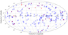 |
Fig. 1. Position of the stars in our sample. The circles represent the stars part of the DEATHSTAR sample while the red stars show the AGB stars in the VLBI sample. |
Properties of the VLBI sources.
3.3. Gaia DR3 parallax
3.3.1. G magnitude and colour
We first investigated the dependence of the Gaia DR3 parallax uncertainties and the parameters that represent the goodness-of-fit of the astrometric data on the G magnitude, and the colour GBP − GRP for the sources in the VLBI sample (Fig. 2) and in the DEATHSTAR sample (Fig. 3). It is apparent in Figs. 2 and 3 that the fainter the star, the redder it is and the smaller its parallax, as expected. However, this behaviour breaks down for the faintest stars (G ≥ 12 mag). The nominal fractional parallax error seems mostly reasonable (below 20%) for sources brighter than G = 8 mag, but shows a slight increase between 8 and 12 G magnitudes. For the three faintest sources in the VLBI sample, the standard Gaia DR3 parallax error is larger than 75% (Fig. 2), while a wider scatter is observed for the faintest stars in the DEATHSTAR sample (Fig. 3). The astrometric excess noise worsens with G magnitude, with an obvious general increase above G = 8 mag. It does not show a strong dependence on the colour. The RUWE does not strongly correlate with neither the colour nor the G magnitude.
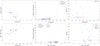 |
Fig. 2. Dependence of the standard noise, the astrometric excess noise, and the RUWE of the Gaia DR3 parallax on the G magnitude and the colour GBP − GRP for the sources in the VLBI sample. |
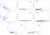 |
Fig. 3. Dependence of the standard noise, the astrometric excess noise, and the RUWE of the Gaia DR3 parallax on the G magnitude and the colour GBP − GRP for the sources in the DEATHSTAR sample. |
We divided the sources in the VLBI and the DEATHSTAR samples into three categories according to their G magnitudes: (1) G < 8, (2) 8 ≤ G < 12, and (3) G ≥ 12 mag. This division is mainly based on the behaviour of their parallax fractional error and the goodness of the Gaia DR3 astrometric measurements measured by their astrometric excess noise, as seen in Figs. 2 and 3.
3.3.2. Zero-point offset and error inflation factor
Figure 4 shows a direct comparison of the VLBI and the Gaia DR3 parallaxes, ϖVLBI and ϖDR3, respectively, for the sources in the VLBI sample. A rather good agreement is observed for the stars with parallaxes lower than 4 mas, with increasing scatter and uncertainties at higher parallax values, corresponding to the brightest sources, along both axes. Figure 4 also shows that the nominal noise of the Gaia DR3 parallaxes,  , is smaller than the VLBI parallax uncertainties
  . However, the uncertainties of the parallaxes measured with Gaia are known to be underestimated, especially for variable objects such as AGB stars. The previously mentioned astrometric excess noise was introduced in DR2 as the extra uncertainty that must be added in quadrature to the nominal noise to obtain a statistically acceptable astrometric solution for Gaia DR2 measurements (Lindegren et al. 2012). A comparative study was conducted by van Langevelde et al. (2018) using Gaia DR2 and VLBI measurements for a number of sources including Mira variables, pre-main sequence stars, and binary pulsars. van Langevelde et al. (2018) attribute the large residual in the Gaia parallaxes to the effects of the properties, such as the colour and surface brightness distribution, of the AGB stars in their sample. Their study confirms that adding the astrometric excess noise of the Gaia measurements to the nominal noise equalises the Gaia DR2 parallaxes with the more robust VLBI measurements.
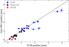 |
Fig. 4. Comparison between the VLBI and Gaia DR3 parallaxes. The solid line represents the 1-to-1 relation. |
In this work, we calibrated the Gaia DR3 parallaxes for AGB stars using the sample of VLBI sources described in Sect. 3.2, which is larger than, and includes, the sample of van Langevelde et al. (2018). To that end, we normalised the distribution of the difference Δϖ= ϖDR3 − ϖVLBI by the sum of the uncertainties in quadrature. We then adjusted the Gaia DR3 uncertainties until that normalised statistical distribution of the parallax difference had the properties of a standard Gaussian, with 0 mean and a standard deviation of 1, as illustrated by Fig. 5. This was done for the three categories described in Sect. 3.3.1. The correction factor to be applied to the Gaia DR3 parallax errors or the error inflation factor (EIF), that is,
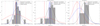 |
Fig. 5. Gaussian fittings of the parallax difference distribution Δω/σϖ, tot for the three G magnitude categories. The distributions were normalised by the quadratically summed errors of the VLBI error with either: the DR3 parallax standard error without any correction ( |

and the zero-point offset (ZPO) of the parallax,

are given in Table 2. Figure 5 also shows the cases where no correction was applied to the total error, that is,  mas, and where the astrometric excess noise was added to the Gaia standard errors,
  mas, as in van Langevelde et al. (2018). Since the distribution of the parallax difference shown in Fig. 5 was normalised by the total error, only taking into account the standard Gaia DR3 uncertainties without any correction led to an underestimation of the total error, resulting in a parallax difference distribution broader than the standard Gaussian for the sources brighter than G = 12 mag. However, including the astrometric excess noise parameter to the total uncertainty of the Gaia DR3 parallax of these bright sources overestimated the total error, which led to a narrower parallax difference distribution (Δϖ/σϖ, tot), as indicated by the blue line in Fig. 4. Furthermore, Fig. 6 shows that the astrometric excess noise parameter for Gaia DR3 is larger than for the DR2 parallaxes for the VLBI sources. The median value of the ratio of astrometric excess noises DR3/DR2 for the VLBI sample is 1.22, and 76% of the sources have an astrometric excess noise DR3/DR2 ratio larger than 1. For the DEATHSTAR sample, close to 60% of the sources have an astrometric excess noise higher in DR3 than in DR2.
Gaia DR3 parallax zero-point offset (ZPO) and error inflation factor (EIF).
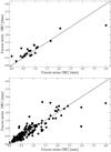 |
Fig. 6. Comparison between the astrometric excess noise of Gaia DR2 and DR3 for the VLBI sample (top) and the DEATHSTAR sample (bottom). The solid lines show the 1-to-1 relation. |
Our results show that the parallax errors of the brightest sources (G < 8) are dramatically underestimated, by more than a factor of 5. For sources between 8 and 12 G mag, the nominal errors are larger, so a relatively smaller correction was needed. For the faintest stars, the nominal Gaia DR3 parallax errors are, in principle, already very large, so little correction was needed on the Gaia DR3 parallax errors. For some of these faint sources, the Gaia DR3 parallax errors are so large that they would have needed to be reduced to recover the corresponding VLBI parallaxes. Distances obtained with parallaxes with such large errors are likely to be very uncertain (see Sect. 4). Only 3 VLBI sources are fainter than 18 mag, which is a too small sample to obtain statistically significant results. Therefore, we did not apply any correction to the faintest stars (G ≥ 12 mag). When considering the VLBI sample as a whole (33 stars), we obtained a constant EIF of ∼4. However, it is clear from Figs. 2 and 3 and Table 2 that not all sources require the same correction factor, so a constant EIF is not suitable.
Using the properties of resolved binaries to calibrate the Gaia eDR3 parallaxes, El-Badry et al. (2021) found that the published Gaia eDR3 parallax uncertainties are underestimated by ∼30 to 80% for bright red sources (G < 12 mag), but are generally more reliable for fainter sources (G ≥ 18 mag), which is in agreement with our findings on AGB stars. The dependence of the parallax ZPO of the Gaia eDR3 parallaxes on the sky position and magnitude are discussed in detail in Lindegren et al. (2021) and Groenewegen (2021), for instance, using samples of quasi-stellar objects and wide binaries. The zero-point offsets that we obtained for AGB stars, listed in Table 2, are much larger, in absolute value, than the global eDR3 zero-point offset of −0.028 mas derived by Ren et al. (2021), and of −0.039 mas by Groenewegen (2021).
4. From parallax to distance
The distance r of an object is equal to the inverse of its true parallax ϖTrue. Assuming that the measured parallax ϖ is a value taken from a normal distribution around the true parallax ϖTrue = 1/r, with a known standard deviation σϖ, the likelihood of that measured parallax is given by
![$$ \begin{aligned} P\,(\varpi \, \vert \, r, \sigma _\varpi ) = \frac{1}{\sqrt{2 \pi }\, \sigma _\varpi } \, \mathrm{exp} \left[-\frac{1}{2\,\sigma _\varpi ^2} \left(\varpi - \frac{1}{r}\right)^2\right], \end{aligned} $$](/articles/aa/full_html/2022/11/aa43670-22/aa43670-22-eq16.gif)
where σϖ > 0. Bailer-Jones (2015) showed that determining the distance from a probability distribution over the parallax presents several problems including negative parallaxes, in particular when the fractional error on the parallax is large (Luri et al. 2018). A better approach is to infer the most probable value of the distance amongst all its possible values from the noisy measured parallax (Bailer-Jones 2015; Astraatmadja & Bailer-Jones 2016a,b; Bailer-Jones et al. 2018, 2021). Such a posterior probability distribution over the distance is the product of the likelihood of the measurement, P (ϖ | r, σϖ), and an appropriate prior information on the distance, P(r). Following Bayes theorem,
where Z is a normalisation constant independent of the distance,
The value of the most probable distance is given by the median of the posterior distribution (Bailer-Jones et al. 2021). The resulting distance uncertainties are asymmetrical because of the non-linear nature of the 1/ϖ to r transformation.
The determining factor in this distance inference problem is the fractional error on the parallax. For a parallax fractional error higher than 20%, the posterior over the distance is highly asymmetrical (Bailer-Jones 2015). This effect worsens with increasing fractional error which results in a non-negligible increase in the value of the derived distance and its uncertainties, and therefore leads to less reliable distances. About 63% of the sources published in eDR3 have parallax fractional errors larger than 20% (Bailer-Jones et al. 2021).
We calculated the posterior distribution over the distance for the sources in the VLBI and the DEATHSTAR samples. In that process, the choice of the prior was paramount. The more assumptions are introduced into the prior, the more model-dependent the resulting distances are, especially when the errors involved are large. Therefore one should choose a prior that closely represents the expected data. To this end, we tested four different priors: a uniform distribution (UD) prior defined in Bailer-Jones (2015) as
a uniform space distribution (USD) prior that is corrected for increasing volume, following the definition given by Bailer-Jones (2015)
an exponentially decreasing space distribution (EDSD) prior that exponentially decreases to 0 as the distance increases, given by
(Bailer-Jones 2015), with L = 250 pc; and a more realistic prior that describes the Galactic distribution of AGB stars (AGB prior). According to Jura & Kleinmann (1990, 1992), the distribution of AGB stars in the Galaxy follows a vertical scale height up to Z0 = 240 pc, and a disc scale length set at R0 of 3500 pc. The AGB prior is also corrected for increasing volume, so that
where RGal is the distance to the Galactic centre and z the height above the Galactic plane.
By checking the 2MASS K-band magnitudes of our sample, we found an apparent K-band limit of 3.2 mag. Assuming that the tip of the AGB is at V = −2 for a solar-mass star, and taking an average of (V − K)=8 from theoretical estimates (Bladh et al. 2013), we obtained a maximum distance estimate of 4400 pc. We therefore limited the allowed distances rmax for the sources in our sample to rmax = 4500 pc.
The Galactic distribution that defines the AGB prior used in this work, based on the findings of Jura & Kleinmann (1992), is in agreement with the Galactic distribution derived by Ishihara et al. (2011) who investigated the difference between the distribution of AGB stars in the Milky Way for the M- and C-type stars. They found a concentration of oxygen-rich stars toward the Galactic centre, with a density decreasing with Galactocentric distance, and a rather uniform distribution within about 8 kpc of the Sun for carbon-rich AGB stars. Jackson et al. (2002) found a distribution that follows a vertical scale height up to 300 pc and a constant number of AGB stars in the radial direction, up to 5 kpc, above which the density decreases exponentially with a scale length of 1.6 kpc, extending to ∼12 kpc. The scale length that we adopted in the AGB prior is consistent with the results of both studies. Varying the scale height Z0 or scale length R0 did not significantly change the derived distances (less than 10% of deviation). The only parameter that affected the derived distances, mostly for the farthest stars, was the maximum allowed distance rmax. Lowering its value led to an increase in the number of sources whose distances were stuck at that upper limit because the posteriors could not reach convergence. Increasing rmax to 5000 pc only changed the distance of two of the stars in the DEATHSTAR sample, putting them at that new upper limit, implying that the distances to these sources are very poorly constrained.
We find that parallax fractional errors larger than ∼18% already lead to notable errors in the derived distances (≳20% distance error with the AGB prior) for some of the sources. More significant uncertainties are associated with parallax fractional errors greater than the previously mentioned 20% cutoff. About 85% of the VLBI sample have a Gaia DR3 parallax fractional error smaller than 0.2 when considering the standard error, but that number decreases to ∼35% after applying the correction to the Gaia DR3 parallaxes derived in Sect. 3. In the case of the DEATHSTAR sample, 94% of the sources have a fractional parallax error lower than 20% before correction, which decreases to ∼52% after correcting the errors on the DR3 parallaxes (see Table A.1).
As expected, the distances derived with the VLBI parallaxes are mostly unchanged with the four priors due to the low measurement uncertainties, as illustrated in Fig. 7. The fractional errors on the VLBI parallaxes are lower than 20% for almost all the sources. In such cases, the posterior distribution is dominated by the likelihood of the data, and the choice of prior does not change the derived distances. The uncertainties on the derived distances are also mostly smaller than 20%, showing their high level of reliability.
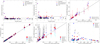 |
Fig. 7. Gaia DR3 and VLBI parallaxes with the corresponding distances for the VLBI sample. Top panels: fractional errors of the VLBI (black full triangles) and Gaia DR3 parallaxes using the standard nominal error (blue open diamond) and with the corrected errors (red full circles) for the VLBI sources. The plot in the middle is a zoomed version of the plot on its left. The plot on the right compares the distances derived with Gaia DR3 parallaxes with the corrected (red) and the standard errors (blue). Bottom panels: distances derived using the four priors for the VLBI sources using the VLBI parallaxes (left) and the corrected Gaia DR3 parallaxes (middle). The solid lines represent the 1-to-1 relation. The plot at the bottom-right shows the fractional error on the derived distances. |
The distances derived with the corrected Gaia DR3 parallaxes are strongly dependent on the prior, as the latter dominates the posterior at large parallax fractional errors. The effects of the value of the parallax fractional errors on the derived distances are illustrated in Figs. 7 and 8, showing comparisons between the Gaia DR3 distances obtained with the different priors, and using the standard and the corrected errors of the Gaia DR3 parallaxes for the sources in the VLBI (Fig. 7) and the DEATHSTAR samples (Fig. 8).
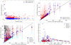 |
Fig. 8. Gaia DR3 parallaxes and the corresponding distances for the DEATHSTAR sample. Top panels: fractional errors of the Gaia DR3 parallaxes using the standard nominal error (blue open diamond) and with the corrected errors (red full circles) for the DEATHSTAR sources. The right plot compares the distances derived with Gaia DR3 parallaxes with the corrected (red) and the standard errors (blue). Bottom panels: distances derived with the four priors for the DEATHSTAR sources using the corrected Gaia DR3 parallaxes. The solid lines represent the 1-to-1 relation. The plot on the right shows the fractional error on the corrected Gaia DR3 distances. |
In the following, we focus on the distances estimated using the AGB prior, as it is more informative and realistic. It is also more sensitive than the other priors we tested because of the larger number of parameters in it. The larger the uncertainties, the higher the probability for the true parallax to be smaller than the measured parallax. As a result, our estimate of the true distance increases. This is known as the Lutz-Kelker bias (Lutz & Kelker 1973). The fractional error on the measurements and the sensitivity of the prior determine how bad the effects are, which means that even nearby objects can be affected. The large errors on the parallaxes lead to significant errors on the derived distances, making them unreliable. Using the corrected Gaia DR3 parallaxes and the AGB prior, we found that about 46% of the sources in the DEATHSTAR sample have distance fractional errors larger than 25%, while more than 15% of them have distance fractional errors greater than 50%. When the prior and/or the posterior distribution did not converge or when the uncertainty on the derived distance was too large, we rejected the derived distance.
5. A new PL relation for Miras
A number of the distances derived with the corrected Gaia DR3 parallaxes following the method described in Sect. 4 are highly uncertain for the sources in the DEATHSTAR sample, and thus rejected. Therefore, we turned to a different method to estimate the distances to these sources: the PL relation. We derived a new bolometric PL relation based on the VLBI distances of the Mira variables in the VLBI sample.
5.1. Derivation
The luminosity of the sources in the VLBI sample were obtained by modelling their spectral energy distributions (SEDs) using the radiative transfer code DUSTY (Ivezic et al. 1999). DUSTY solves the radiative transfer through a dusty environment including dust absorption, emission, and scattering. The details of the SED fitting are given in Appendix B. From the dust modelling, we obtained the effective temperature of the central star, T⋆, the dust temperature at the inner radius, Td, the optical depth at 10 μm, τ10, and the bolometric luminosity, L⋆, of each source in the VLBI sample. These results are listed in Table 3.
DUSTY results for the VLBI sources.
The bolometric magnitude Mbol of each star was calculated (assuming Mbol, ⊙ = 4.74) and correlated with the variability period which was taken either from the GCVS (Samus’ et al. 2017) or the International Variable Star Index (VSX; Watson et al. 2021). We removed from the PL relation derivation the sources that are known or suspected not to behave as regular Mira variables. The OH/IR stars in the VLBI sample were, therefore, excluded from this analysis. These stars lie at the end of the evolution of the AGB and have very high mass-loss rates (Herman et al. 1985). They have been found to consistently lie below the PL relation of typical Miras (van Langevelde et al. 1990; Whitelock et al. 1991). The stars in our VLBI sample labelled as OH/IR in the SIMBAD database are NSV 17351, QX Pup, and SY Aql. In addition, OZ Gem has recently been suspected as being in the process of becoming an OH/IR star (Urago et al. 2020). The study conducted by Chibueze et al. (2020) suggests that AP Lyn could undergo the same process as OZ Gem due to its high mass-loss rate. Finally, we also excluded FV Boo and UX Cyg from the Mira-PL relation determination. Lewis (2002a,b) described FV Boo as a dying OH/IR star, with a mass loss that abruptly switches on and off. Monitoring of FV Boo in the IR over a 20-year span by Kamezaki et al. (2016b) showed that it suffered a temporary but significant dip in its luminosity in 2005. The star UX Cyg stood out in the sample of Mira variables investigated by Etoka & Le Squeren (2000) due to rapid, large changes in the amplitude of the variations of its maser lines, likely linked to an unusually turbulent envelope. Whitelock et al. (2008) excluded UX Cyg from their K-band PL relation as they hypothesised it to be either an overtone pulsator or a hot bottom burning candidate.
We used the form of the PL relation introduced by Whitelock et al. (2008) where the zero-point is shifted within the range of typical periods of Mira variables. The resulting PL relation has a slope of −2.67 ± 1.88 and a zero-point of 2.323 ± 4.832. The large errors are due to the small sample size. This problem can be solved by using a fixed slope and by keeping the zero point as only free parameter. Using stars in the Large Magellanic Cloud (LMC) and in the Milky Way, Whitelock et al. (2008) showed that, while the zero-point differs for oxygen-rich and carbon stars, the slope of the K-band PL relation is nearly invariant. In addition, using a common fixed slope for the Milky Way and the LMC, Whitelock et al. (2008) showed that the zero-point of the K-band PL relation for Mira variables in these two different environments were consistent with each other within their uncertainties, implying that the K-band PL relation is universal. This property of universality was then extended to the bolometric PL relation by Whitelock et al. (2009), where they determined the distance to the Fornax Galaxy using a bolometric PL relation derived in the LMC. Accordingly, with the assumption that the slope invariance with chemical type is also applicable to the bolometric PL relation, we use the slope of  derived for C-stars in the LMC by Whitelock et al. (2009). We obtain the PL relation given by
![$$ \begin{aligned} M_{\rm bol} = (-3.31\pm 0.24)\,[\mathrm{log}\, P - 2.5] + (-4.317\pm 0.060). \end{aligned} $$](/articles/aa/full_html/2022/11/aa43670-22/aa43670-22-eq32.gif)
The zero-point derived in this work for M-type stars reasonably agrees with existing bolometric PL relations for C-stars both in the LMC (Whitelock et al. 2006, 2009) and in the Milky Way (Feast et al. 2006), as seen in Fig. 9. In particular, our PL relation is in excellent agreement with the zero-point of the PL relation of Whitelock et al. (2009). Whitelock et al. (2008, 2009) compared the luminosity obtained from interpolating IR measurements with the luminosity derived from dust modelling using DUSTY (e.g. Matsuura et al. 2007) and concluded that the latter could be overestimated by up to 50%. On the other hand, bolometric magnitudes in Whitelock et al. (2006, 2009) were estimated by integrating under a spline curve fitted to fluxes at J, H, K, L, 12, and 25 μm. The curve was extrapolated at the end points to reach zero flux at zero frequency at the short end (long end in wavelength) and by joining the K-band flux with zero flux through a point between the H and K fluxes, which could have underestimated the total luminosity. However, the bolometric magnitude obtained with the PL relation derived in this work is only about 0.046 mag brighter than in Whitelock et al. (2009), and 0.048 mag fainter than the bolometric magnitudes obtained by Whitelock et al. (2006), on average. Furthermore, although the associated uncertainties are very large because of the small sample size, the PL relation we derived with a non-fixed slope appears, in general, to be consistent with the PL relation derived by Whitelock et al. (2006) (see Fig. 9). As expected, most of the (candidate/dying) OH/IR stars lie below the derived PL relation, with the exception of NSV 17351.
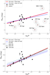 |
Fig. 9. Derived PL relation for Mira variables. Top: bolometric PL relation based on the luminosity of the Mira variables in the VLBI sample. The red solid line shows the PL relation obtained when using a fixed slope, and the blue dashed line represents the relation obtained when the slope is a free parameter. The sources excluded from the fit are represented by the open symbols. Bottom: comparison between our PL relation with the bolometric PL relations for C-type stars by Feast et al. (2006) in the Milky Way (F06 MW), Whitelock et al. (2006) (W06 LMC), and Whitelock et al. (2009) (W09 LMC) in the LMC. |
5.2. The universality of the PL relation
As previously mentioned, Whitelock et al. (2008) demonstrated that the PL relation is universal. This was proven by the good agreement between the zero-points of the PL relations in the LMC, the Milky Way, and the Fornax dwarf Galaxy, assuming a common slope. However, recent studies by Urago et al. (2020) and Chibueze et al. (2020) have cast doubt on the universality of the PL relation in environments with different metallicities. Their conclusion of a non-universal PL relation comes from the position of the Galactic oxygen-rich star OZ Gem on the LMC K-band PL diagram. Given its luminosity, chemistry, and high mass-loss rate implied by its very red colour, Urago et al. (2020) concluded that OZ Gem is likely an OH/IR star. Their photometric measurements, however, placed OZ Gem on the region for C-stars on the K-band PL relation in the LMC, below the line for M-type stars (see their Fig. 9). Our results show that OZ Gem also lies below the bolometric PL relation for Mira variables in the Milky Way (see Fig. 9). This corroborates the results of Urago et al. (2020) on the OH/IR nature of this source, as OH/IR stars tend to have low luminosity for their relatively long period (e.g. Fig. 10 in Whitelock et al. 1991) compared to typical Miras. They are also expected to be less luminous in the K-band because of dust obscuration from their thick CSE. In other words, OZ Gem is an outlier even amongst the Mira variables in the Milky Way and its position in the (K-band or bolometric) PL relation does not represent the general trend for the typical Mira variables in the Galaxy. This interpretation, therefore, does not invalidate the universality of the PL relation for regular Miras. However, the absence of typical oxygen-rich Miras at longer periods (> 600 days) is apparent in Fig. 9, as they are expected to be either brighter due to hot bottom burning, or fainter due to high mass-loss rates (e.g. OH/IR stars). There is, however, no such gap at longer periods in the K-band PL relation of oxygen-rich stars in the LMC. The apparent absence of regular oxygen-rich Miras at longer periods in the Milky Way could indicate that the universality of the PL relation with metallicity breaks down at long periods for oxygen-rich Miras.
6. A new distance catalogue
In this section, we present a new distance catalogue for the ∼200 sources in the DEATHSTAR sample, based on our results in Sects. 3–5, and using alternative methods in the literature when applicable, as described below. Table C.1 gives the distances and the associated uncertainties for the nearby AGB stars in the DEATHSTAR sample. The displayed distances are estimated using the following methods.
For the AGB stars in the VLBI sample, we estimated the distances and their errors using the VLBI parallaxes (Type = V in Table C.1), following the Bayesian approach using the AGB prior described in Sect. 4. The corresponding distances have fractional errors within 25%. For the sources outside the VLBI sample that have a corrected Gaia DR3 parallax fractional error below 15%, the best distance estimate listed in Table C.1 is the Gaia DR3 distance obtained with the AGB prior (Type = GAGB). For sources with a corrected Gaia DR3 parallax fractional error between 15 and 20%, we checked if the fractional error on the distance derived using the Bayesian approach with the AGB prior is within 25%. If that condition was fulfilled, the distance in Table C.1 is the Gaia DR3 distance with AGB prior (Type = GAGB). Otherwise, the distance was determined using a PL relation, provided that the source had a known period and variability type. The PL relation derived in Sect. 5,
![$$ \begin{aligned} M_{\rm bol} = (-3.31\pm 0.24)\,[\mathrm{log}\, P - 2.5] + (-4.317\pm 0.060), \end{aligned} $$](/articles/aa/full_html/2022/11/aa43670-22/aa43670-22-eq33.gif)
was used to derive the luminosity of the Mira variables (Type = PL(M) in Table C.1). We then performed radiative transfer modelling of the stellar and dust emission, as in Sect. 5, to determine their distances. The details of the dust modelling are given in Appendix B. It is important to note that this PL relation was derived using Mira variables with periods between 277 and 514 days, so the distances for the sources outside this range derived with this relation (Type = PL(Mout)) can be less reliable. However, given the good agreement between our PL relation and existing PL relations for Miras that are valid within a wider period range, ∼160 − 930 days for Feast et al. (2006), for instance, using our PL relation for sources within that wider range of periods is a reasonable first approximation.
For semi-regulars (SRs), we used the PL relation from Knapp et al. (2003) given by

to estimate the absolute magnitudes of the sources in the K-band. The distance was obtained using the distance modulus relation (Type = PL(SRa/b) in Table C.1). The apparent magnitude in the K-band was retrieved from the VSX online search tool (Watson et al. 2021). Interstellar extinction in the K band is expected to be low. For the sources in our sample that are also in Knapp et al. (2003) or Whitelock et al. (2008), we used the AK coefficients calculated by Knapp et al. (2003) or the AV (lower limits) in Whitelock et al. (2008) for these individual sources to correct for reddening. Otherwise, we assumed a value of AK = 0.02 mag, representing the mean value of the AK distribution in Knapp et al. (2003). The use of a single PL relation for SRs is motivated in the literature by the fact that they are possible progenitors of Mira variables, so some sort of similarity in their behaviour is expected (Feast & Whitelock 2000). The PL relation for SRs by Knapp et al. (2003) that we used here is in good agreement with the relation derived by Yeşilyaprak & Aslan (2004) for SRs, within their respective uncertainties. However, as SRs, SRbs in particular, are less regular and have lower amplitude, their pulsation behaviour is less well-understood than Mira variables, and their period and luminosity show a weaker correlation. In addition, studies such as Soszyński et al. (2013) showed that SRs can have more than one pulsation period and lie on different PL sequences. Therefore, the reliability of the distances derived with this method can be arguable. More recently, Trabucchi et al. (2021) investigated the suitability of SRs as distance indicators and found that a subgroup of SRs follows the same sequence as Mira variables in the PL diagram. However, they concluded that long-time series are necessary to properly classify SRs according to their pulsation periods. The study of the variability of SRs is beyond the scope of this paper. Finally, for the remaining sources in the DEATHSTAR sample with corrected Gaia DR3 parallax fractional error larger than 20%, we estimated the distance with a PL relation, depending on the variability type, as described above.
We note that the distances presented in this catalogue were derived in a systematic way for the whole DEATHSTAR sample. For some sources, however, independent and more accurate source-specific distances obtained with the phase-lag method are available in the literature. This is the case, for example, for IRC+10216 (123 ± 14 pc; Groenewegen et al. 2012), R Scl (361 ± 44 pc; Maercker et al. 2018), and OH/IR stars (e.g. Herman et al. 1985; Engels et al. 2015; Etoka et al. 2018). Our distance of 408 pc for R Scl agrees rather well with its phase-lag distance. The distance of 190 ± 20 pc that we derived for IRC+10216 with our PL relation for Miras is consistent within 3σ with its distance derived by Groenewegen et al. (2012), but the error is, nonetheless, relatively large. This can be due to the fact that the period of IRC+10216 lies outside the period range with which our PL relation was derived. This shows that one should be careful when using the PL(Mout) distances in Table C.1, as the displayed errors do not account for uncertainties related to the longer/shorter periods of these sources.
6.1. Comparing the corrected Gaia DR3 and the PL distances
We considered the sources that have ‘good’ Gaia DR3 distances, which are distances with fractional errors below 25%. For comparison purposes, we also derived alternative distances for these same sources, using either the PL relation that we developed in Sect. 5 for the Miras, or the PL relation by Knapp et al. (2003) for the SRs. Figure 10 shows that, for the Miras, the distances derived with the two methods are in good agreement, considering their respective uncertainties. The only notable exception is the carbon star LP And, whose derived PL distance is about 4 times larger than its Gaia DR3 distance. The nominal Gaia DR3 parallax fractional error of LP And is about 10%, but the corresponding astrometric excess noise is almost as large as the value of its parallax (∼99%). Moreover, LP And is a very faint star, with a magnitude of G = 17.6 mag. As we did not apply any correction to the parallax error of such faint stars, the parallax fractional error that we used to calculate the Gaia distance of this source could be underestimated. On the other hand, LP And has a period of 614 days, outside the range of periods with which we derived our Mira PL relation, which could have led to this observed discrepancy. The good agreement between the derived Gaia DR3 and PL distances for the Miras in Fig. 10, within their respective uncertainties, demonstrates the reliability of our new PL relation based on the VLBI distances for Mira variables. The distances of some of the SRs derived with the PL relation by Knapp et al. (2003) are slightly deviant from the corrected Gaia DR3 distances, some differing by ≥50%. There is no clear distinction between the SRas and SRbs. This discrepancy in the two methods is likely due to uncertainties related to the complex pulsation behaviour of these SRs and highlights the need for a better-constrained PL relation for these sources.
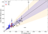 |
Fig. 10. Comparison between the ‘good’ Gaia DR3 distances (see text) and the PL distances for the same sources. The black line shows the 1-to-1 relation. The blue and orange regions show the range of ±25 and ±50%, respectively. |
6.2. Comparison with the NESS catalogue
A new distance catalogue for evolved stars was recently published by Scicluna et al. (2022) as part of the Nearby Evolved Stars Survey (NESS5). The NESS catalogue comprises distances for more than 800 stars, including AGB stars as well as other giants and supergiants. Their distances for AGB stars that are beyond ∼400 pc are based on a new metric derived from the luminosity probability distribution of AGB stars in the LMC. In addition, the NESS catalogue provides distances based on previous maser, Tycho-Gaia Astrometric Solution (TGAS) of Gaia Data Release 1 (DR1), and HIPPARCOS inverted parallaxes, with parallax fractional errors within 25%. About 55% of the sources in the DEATHSTAR sample have distances in the NESS catalogue, mainly based on their new luminosity distance metric (∼37%), HIPPARCOS data (∼16%), and previous maser measurements (∼2%). Figure 11 shows that the NESS luminosity distances agree reasonably well with the distances that were derived in this work, in particular for sources within 750 pc (in our distance). The errors on the NESS luminosity distances are fixed to 25% for all sources, whereas the fractional errors on the distances that we derived change from source to source and are below 25% for all the sources that are in both the NESS and the DEATHSTAR samples.
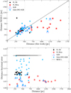 |
Fig. 11. Comparison with the NESS luminosity distance. Top: the NESS luminosity distance (L) compared with the distances calculated with the various methods used in this work. The black line shows the 1-to-1 relation. Bottom: the distance fractional errors obtained in this work and those derived with the NESS luminosity distance. |
6.3. RUWE
The re-normalised unit weight error or RUWE was introduced by Lindegren (2018) for Gaia DR2 and is a measure of the goodness-of-fit of astrometric data. As previously mentioned, the RUWE and the astrometric excess noise both measure discrepancies due to photocentric motions. The astrometric excess noise is expressed as an angle with an ideal value of 0 mas for a good fit, while the RUWE is dimensionless, with an ideal value of 1.0 for well-behaved sources. A value of RUWE ≤1.4 is the criterion for good astrometric solutions. Lindegren (2018) obtained that 1.4 good-fit criterion by looking at the shape of the distribution of RUWE for a sample of 338 833 sources within 100 pc of the Sun. In their work, the distribution of RUWE follows a normal distribution that peaks at approximately 1.0, but exhibits a long tail towards higher values, with a breakpoint at RUWE ≃1.4.
The distribution of the RUWE of the sources in the DEATHSTAR sample that have a Gaia DR3 distance fractional error within 25% has a shape similar to the distribution in Lindegren (2018), as seen in Fig. 12, with a median value of ∼1.2 and a tail reaching a maximum RUWE of ∼4.8. The RUWE of about 40% of these sources whose derived Gaia distances are reliable are smaller than or equal to 1.4. Although the RUWE of the sources with distance fractional errors larger than 25% can reach higher values (∼8.8), more than 20% of these sources have a RUWE within the 1.4 good-fit criterion. Therefore, a RUWE value of 1.4 does not guarantee reliable distance estimates, and we caution against the use of only the RUWE to assess the quality of astrometric data from Gaia DR3 for AGB stars. Figure 12 also shows that, irrespective of the RUWE, bright stars (G < 8 mag) are dominant in the sample of sources with distance fractional error larger than 25%. There is no clear trend with the distance fractional error and the colour.
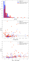 |
Fig. 12. Assessment of the RUWE criterion. Top: distribution of the RUWE of the sources in the DEATHSTAR sample for the ‘good’ (blue) and ‘bad’ (red) derived Gaia DR3 distances. Middle: RUWE of the sources in the DEATHSTAR sample as a function of G magnitude, where the blue open circles and the red full circles represent distances with fractional error within and above 25%, respectively. Bottom: RUWE of the sources in the DEATHSTAR sample as a function of colour. The symbols are the same as above. |
Lindegren (2018) found that the RUWE parameter is most useful to assess the quality and reliability of the astrometric data of samples that include extremely bright, red or blue sources. However, the results of Fabricius et al. (2021) showed that the RUWE value in Gaia DR3 for bright sources in crowded areas is strongly underestimated. The RUWE can be used to detect unresolved binaries (Lindegren et al. 2021). Stassun & Torres (2021) found that, due to its high sensitivity to photocenter motions, a RUWE that is even slightly greater than 1.0 may indicate the presence of unresolved binaries. About 78% of the sources in the DEATHSTAR sample have a RUWE higher than 1.0. For AGB stars, however, a high RUWE is more likely caused by saturation of the detector, the large size of the star, and/or the photocentre shift caused by convective motions on the stellar photosphere.
7. Summary and conclusions
A number of studies have shown that the parallaxes of AGB stars measured with Gaia are bound to have large errors, as their intrinsic properties bring additional uncertainties to the parallax measurements (circumstellar dust, colour, large size, and surface brightness variability; Chiavassa et al. 2018; Xu et al. 2019; El-Badry et al. 2021). Deriving distances from parallaxes in general is not a straightforward process, and the large errors of the parallaxes of AGB stars make it even more complicated. In this work, we assessed the Gaia DR3 parallaxes and the corresponding distances for two samples of nearby AGB stars, the DEATHSTAR and the VLBI samples. Our main results can be summarised as follows.
The standard errors of the Gaia DR3 parallaxes are underestimated by more than a factor of 5 for the brightest sources (G < 8 mag), based on a comparison with the more robust VLBI parallaxes. Introducing the astrometric excess noise in the total error, as was done for Gaia DR2, would overestimate the uncertainties. The excess noise for DR3 is higher than the DR2 excess noise for ≥60% of the sources in both samples.
We inferred distances from parallaxes using a Bayesian approach that follows the procedure in Bailer-Jones (2015). This method requires the use of a prior that provides information on the distances. The best prior is one that uses all available information on the sources in order to obtain the most realistic distances. We introduced the AGB prior which follows the Galactic distribution of AGB stars by Jura & Kleinmann (1990), with a scale height of 240 pc and a scale length of 3500 pc. The most important parameter in this inference problem is the fractional error on the measured parallaxes. Our results confirmed the higher limit on the parallax fractional error of 0.2 stated by Bailer-Jones (2015) for good measurements. Below that limit, the posterior distribution of the distance is closely related to the likelihood of the measurements and to 1/ϖ. This was the case for the VLBI sample and more than half of the DEATHSTAR sample, using the corrected Gaia DR3 parallaxes. For the remaining sources with fractional errors above 0.2, the posterior is dominated by the prior, and the errors on the distances are usually large and asymmetrical. The AGB prior, although representative of the distribution of AGB stars, is highly sensitive to the level of fractional noise, and some cases of non-convergence were observed due to the constraints imposed by the prior. The estimated distances present large uncertainties when the fractional parallax errors are large, irrespective of the prior used. They are also less likely to be close to the values given by 1/ϖ. It is important to note that the measured parallax ϖ is not the true parallax, and adopting the distance as the inverse of the measured parallax is not reliable.
The radiative code DUSTY was used to determine the luminosity of the VLBI sources using the better-constrained distances obtained with the VLBI parallaxes. We used the calculated luminosities to derive a new bolometric PL relation for oxygen-rich Mira variables in the Milky Way, valid for periods between 276 and 514 days. We obtained a PL relation of the form Mbol = (− 3.31 ± 0.24) [log P − 2.5]+(−4.317 ± 0.060). The PL relation for M-type Mira variables in the Galaxy derived in this work does not significantly differ from existing bolometric PL relations for C-type Miras in the LMC and in the Milky Way (e.g. Feast et al. 2006; Whitelock et al. 2006, 2009).
We provided a new distance catalogue for about 200 nearby AGB stars estimated from VLBI and corrected DR3 Gaia parallaxes, and PL relations for Mira (this work) and SR (Knapp et al. 2003) variables. Finally, we caution against the use of the RUWE parameter as the sole measure of the quality of Gaia DR3 astrometric data for individual AGB stars, as a RUWE below 1.4 does not guarantee reliable distance estimates.
Acknowledgments
The authors are grateful to Kjell Eriksson for computing the MARCS models, and Sara Bladh for the helpful discussions on the stellar spectra for the SED modelling. We thank the referee for their constructive feedback on the manuscript. E.D.B. acknowledges financial support from the Swedish National Space Agency. W.V. acknowledges support from the Swedish Research Council through grant No. 2020-04044. This project has received funding from the European Research Council (ERC) under the European Union’s Horizon 2020 research and innovation programme under grant agreements No. 883867 [EXWINGS]. This work presents results from the European Space Agency (ESA) space mission Gaia. Gaia data are being processed by the Gaia Data Processing and Analysis Consortium (DPAC). Funding for the DPAC is provided by national institutions, in particular the institutions participating in the Gaia MultiLateral Agreement (MLA). The Gaia mission website is https://www.cosmos.esa.int/gaia. The Gaia archive website is https://archives.esac.esa.int/gaia. This research made use of Astropy (http://www.astropy.org), a community-developed core Python package for Astronomy (Astropy Collaboration 2013, 2018). This research has made use of the VizieR catalogue access tool and the SIMBAD database, operated at CDS, Strasbourg, France.
References
- Ahmad, A., Freytag, B., & Höfner, S. 2022, A&A, submitted [Google Scholar]
- Andriantsaralaza, M., Ramstedt, S., Vlemmings, W. H. T., et al. 2021, A&A, 653, A53 [NASA ADS] [CrossRef] [EDP Sciences] [Google Scholar]
- Aringer, B., Marigo, P., Nowotny, W., et al. 2019, MNRAS, 487, 2133 [CrossRef] [Google Scholar]
- Astraatmadja, T. L., & Bailer-Jones, C. A. L. 2016a, ApJ, 832, 137 [NASA ADS] [CrossRef] [Google Scholar]
- Astraatmadja, T. L., & Bailer-Jones, C. A. L. 2016b, ApJ, 833, 119 [NASA ADS] [CrossRef] [Google Scholar]
- Astropy Collaboration (Robitaille, T. P., et al.) 2013, A&A, 558, A33 [NASA ADS] [CrossRef] [EDP Sciences] [Google Scholar]
- Astropy Collaboration (Price-Whelan, A. M., et al.) 2018, AJ, 156, 123 [Google Scholar]
- Bailer-Jones, C. A. L. 2015, PASP, 127, 994 [Google Scholar]
- Bailer-Jones, C. A. L., Rybizki, J., Fouesneau, M., Mantelet, G., & Andrae, R. 2018, AJ, 156, 58 [Google Scholar]
- Bailer-Jones, C. A. L., Rybizki, J., Fouesneau, M., Demleitner, M., & Andrae, R. 2021, AJ, 161, 147 [Google Scholar]
- Bladh, S., Höfner, S., Nowotny, W., Aringer, B., & Eriksson, K. 2013, A&A, 553, A20 [NASA ADS] [CrossRef] [EDP Sciences] [Google Scholar]
- Carrasco, J. M., Evans, D. W., Montegriffo, P., et al. 2016, A&A, 595, A7 [NASA ADS] [CrossRef] [EDP Sciences] [Google Scholar]
- Chiavassa, A., Freytag, B., & Schultheis, M. 2018, A&A, 617, L1 [NASA ADS] [CrossRef] [EDP Sciences] [Google Scholar]
- Chiavassa, A., Kravchenko, K., Millour, F., et al. 2020, A&A, 640, A23 [NASA ADS] [CrossRef] [EDP Sciences] [Google Scholar]
- Chibueze, J. O., Urago, R., Omodaka, T., et al. 2020, PASJ, 72, 59 [NASA ADS] [CrossRef] [Google Scholar]
- El-Badry, K., Rix, H.-W., & Heintz, T. M. 2021, MNRAS, 506, 2269 [NASA ADS] [CrossRef] [Google Scholar]
- Engels, D., Etoka, S., Gérard, E., & Richards, A. 2015, in Why Galaxies Care about AGB Stars III: A Closer Look in Space and Time, eds. F. Kerschbaum, R. F. Wing, & J. Hron, ASP Conf. Ser., 497, 473 [NASA ADS] [Google Scholar]
- Etoka, S., & Le Squeren, A. M. 2000, A&AS, 146, 179 [NASA ADS] [CrossRef] [EDP Sciences] [Google Scholar]
- Etoka, S., Engels, D., Gérard, E., & Richards, A. M. S. 2018, in Astrophysical Masers: Unlocking the Mysteries of the Universe, eds. A. Tarchi, M. J. Reid, & P. Castangia, 336, 381 [NASA ADS] [Google Scholar]
- Fabricius, C., Luri, X., Arenou, F., et al. 2021, A&A, 649, A5 [NASA ADS] [CrossRef] [EDP Sciences] [Google Scholar]
- Feast, M. W., & Whitelock, P. A. 2000, MNRAS, 317, 460 [NASA ADS] [CrossRef] [Google Scholar]
- Feast, M. W., Whitelock, P. A., & Menzies, J. W. 2006, MNRAS, 369, 791 [NASA ADS] [CrossRef] [Google Scholar]
- Freytag, B., Liljegren, S., & Höfner, S. 2017, A&A, 600, A137 [NASA ADS] [CrossRef] [EDP Sciences] [Google Scholar]
- Gaia Collaboration (Prusti, T., et al.) 2016a, A&A, 595, A1 [NASA ADS] [CrossRef] [EDP Sciences] [Google Scholar]
- Gaia Collaboration (Brown, A. G. A., et al.) 2016b, A&A, 595, A2 [NASA ADS] [CrossRef] [EDP Sciences] [Google Scholar]
- Gaia Collaboration (Brown, A. G. A., et al.) 2018, A&A, 616, A1 [NASA ADS] [CrossRef] [EDP Sciences] [Google Scholar]
- Gaia Collaboration (Brown, A. G. A., et al.) 2021, A&A, 649, A1 [NASA ADS] [CrossRef] [EDP Sciences] [Google Scholar]
- Gaia Collaboration (Vallenari, A., et al.) 2022, ArXiv e-prints [arXiv:2208.00211] [Google Scholar]
- González Delgado, D., Olofsson, H., Kerschbaum, F., et al. 2003, A&A, 411, 123 [Google Scholar]
- Groenewegen, M. A. T. 2021, A&A, 654, A20 [NASA ADS] [CrossRef] [EDP Sciences] [Google Scholar]
- Groenewegen, M. A. T., de Jong, T., van der Bliek, N. S., Slijkhuis, S., & Willems, F. J. 1992, A&A, 253, 150 [NASA ADS] [Google Scholar]
- Groenewegen, M. A. T., Barlow, M. J., Blommaert, J. A. D. L., et al. 2012, A&A, 543, L8 [NASA ADS] [CrossRef] [EDP Sciences] [Google Scholar]
- Gustafsson, B., Edvardsson, B., Eriksson, K., et al. 2008, A&A, 486, 951 [NASA ADS] [CrossRef] [EDP Sciences] [Google Scholar]
- Herman, J., Baud, B., Habing, H. J., & Winnberg, A. 1985, A&A, 143, 122 [NASA ADS] [Google Scholar]
- Höfner, S., & Olofsson, H. 2018, A&ARv, 26, 1 [Google Scholar]
- Ishihara, D., Kaneda, H., Onaka, T., et al. 2011, A&A, 534, A79 [NASA ADS] [CrossRef] [EDP Sciences] [Google Scholar]
- Ivezic, Z., Nenkova, M., & Elitzur, M. 1999, Astrophysics Source Code Library [record ascl:9911.001] [Google Scholar]
- Jackson, T., Ivezić, Ž., & Knapp, G. R. 2002, MNRAS, 337, 749 [NASA ADS] [CrossRef] [Google Scholar]
- Jorissen, A., & Knapp, G. R. 1998, A&AS, 129, 363 [NASA ADS] [CrossRef] [EDP Sciences] [Google Scholar]
- Jura, M., & Kleinmann, S. G. 1990, ApJ, 364, 663 [NASA ADS] [CrossRef] [Google Scholar]
- Jura, M., & Kleinmann, S. G. 1992, ApJS, 79, 105 [CrossRef] [Google Scholar]
- Justtanont, K., & Tielens, A. G. G. M. 1992, ApJ, 389, 400 [CrossRef] [Google Scholar]
- Kamezaki, T., Nakagawa, A., Omodaka, T., et al. 2016a, PASJ, 68, 71 [NASA ADS] [CrossRef] [Google Scholar]
- Kamezaki, T., Nakagawa, A., Omodaka, T., et al. 2016b, PASJ, 68, 75 [NASA ADS] [CrossRef] [Google Scholar]
- Knapp, G. R., Pourbaix, D., Platais, I., & Jorissen, A. 2003, A&A, 403, 993 [NASA ADS] [CrossRef] [EDP Sciences] [Google Scholar]
- Kurayama, T., Sasao, T., & Kobayashi, H. 2005, ApJ, 627, L49 [NASA ADS] [CrossRef] [Google Scholar]
- Lewis, B. M. 2002a, Am. Astron. Soc. Meet. Abstr., 201, 25.06 [NASA ADS] [Google Scholar]
- Lewis, B. M. 2002b, ApJ, 576, 445 [NASA ADS] [CrossRef] [Google Scholar]
- Lian, J., Zhu, Q., Kong, X., & He, J. 2014, A&A, 564, A84 [NASA ADS] [CrossRef] [EDP Sciences] [Google Scholar]
- Lindegren, L. 2018, Gaia Data Processing and Analysis Consortium [Google Scholar]
- Lindegren, L., Lammers, U., Hobbs, D., et al. 2012, A&A, 538, A78 [NASA ADS] [CrossRef] [EDP Sciences] [Google Scholar]
- Lindegren, L., Klioner, S. A., Hernández, J., et al. 2021, A&A, 649, A2 [EDP Sciences] [Google Scholar]
- Luri, X., Brown, A. G. A., Sarro, L. M., et al. 2018, A&A, 616, A9 [NASA ADS] [CrossRef] [EDP Sciences] [Google Scholar]
- Lutz, T. E., & Kelker, D. H. 1973, PASP, 85, 573 [Google Scholar]
- Maercker, M., Brunner, M., Mecina, M., & De Beck, E. 2018, A&A, 611, A102 [NASA ADS] [CrossRef] [EDP Sciences] [Google Scholar]
- Matsuura, M., Zijlstra, A. A., Bernard-Salas, J., et al. 2007, MNRAS, 382, 1889 [NASA ADS] [CrossRef] [Google Scholar]
- Nakagawa, A., Omodaka, T., Handa, T., et al. 2014, PASJ, 66, 101 [NASA ADS] [CrossRef] [Google Scholar]
- Nyu, D., Nakagawa, A., Matsui, M., et al. 2011, PASJ, 63, 63 [NASA ADS] [CrossRef] [Google Scholar]
- Olofsson, H., González Delgado, D., Kerschbaum, F., & Schöier, F. L. 2002, A&A, 391, 1053 [NASA ADS] [CrossRef] [EDP Sciences] [Google Scholar]
- Ramstedt, S., Schöier, F. L., Olofsson, H., & Lundgren, A. A. 2006, A&A, 454, L103 [NASA ADS] [CrossRef] [EDP Sciences] [Google Scholar]
- Ramstedt, S., Schöier, F. L., Olofsson, H., & Lundgren, A. A. 2008, A&A, 487, 645 [NASA ADS] [CrossRef] [EDP Sciences] [Google Scholar]
- Ramstedt, S., Schöier, F. L., & Olofsson, H. 2009, A&A, 499, 515 [NASA ADS] [CrossRef] [EDP Sciences] [Google Scholar]
- Ramstedt, S., Vlemmings, W. H. T., Doan, L., et al. 2020, A&A, 640, A133 [EDP Sciences] [Google Scholar]
- Reid, M. J., & Honma, M. 2014, ARA&A, 52, 339 [NASA ADS] [CrossRef] [Google Scholar]
- Ren, F., Chen, X., Zhang, H., et al. 2021, ApJ, 911, L20 [NASA ADS] [CrossRef] [Google Scholar]
- Rouleau, F., & Martin, P. G. 1991, ApJ, 377, 526 [NASA ADS] [CrossRef] [Google Scholar]
- Samus’, N. N., Kazarovets, E. V., Durlevich, O. V., Kireeva, N. N., & Pastukhova, E. N. 2017, Astron. Rep., 61, 80 [Google Scholar]
- Sánchez Contreras, C., Alcolea, J., Rodríguez Cardoso, R., et al. 2022, A&A, 665, A88 [CrossRef] [EDP Sciences] [Google Scholar]
- Schlegel, D. J., Finkbeiner, D. P., & Davis, M. 1998, ApJ, 500, 525 [Google Scholar]
- Schöier, F. L., & Olofsson, H. 2001, A&A, 368, 969 [Google Scholar]
- Scicluna, P., Kemper, F., McDonald, I., et al. 2022, MNRAS, 512, 1091 [NASA ADS] [CrossRef] [Google Scholar]
- Soszyński, I., Wood, P. R., & Udalski, A. 2013, ApJ, 779, 167 [CrossRef] [Google Scholar]
- Stassun, K. G., & Torres, G. 2021, ApJ, 907, L33 [NASA ADS] [CrossRef] [Google Scholar]
- Stephenson, C. B. 1984, A General Catalogue of Galactic S Stars, Publications of the Warner and Swasey Observatory (Cleveland, Ohio: Case Western Reserve University), 3 [Google Scholar]
- Sun, Y., Zhang, B., Reid, M. J., et al. 2022, ApJ, 931, 74 [NASA ADS] [CrossRef] [Google Scholar]
- Trabucchi, M., Mowlavi, N., & Lebzelter, T. 2021, A&A, 656, A66 [NASA ADS] [CrossRef] [EDP Sciences] [Google Scholar]
- Urago, R., Yamaguchi, R., Omodaka, T., et al. 2020, PASJ, 72, 57 [NASA ADS] [CrossRef] [Google Scholar]
- van Langevelde, H. J., van der Heiden, R., & van Schooneveld, C. 1990, A&A, 239, 193 [NASA ADS] [Google Scholar]
- van Langevelde, H., Quiroga-Nuñez, L. H., Vlemmings, W. H. T., et al. 2018, 14th European VLBI Network Symposium& Users Meeting (EVN 2018), 43 [Google Scholar]
- van Leeuwen, F., Evans, D. W., De Angeli, F., et al. 2017, A&A, 599, A32 [NASA ADS] [CrossRef] [EDP Sciences] [Google Scholar]
- VERA Collaboration (Hirota, T., et al.) 2020, PASJ, 72, 50 [Google Scholar]
- Vlemmings, W. H. T., & van Langevelde, H. J. 2007, A&A, 472, 547 [NASA ADS] [CrossRef] [EDP Sciences] [Google Scholar]
- Vlemmings, W. H. T., van Langevelde, H. J., & Diamond, P. J. 2002, A&A, 393, L33 [NASA ADS] [CrossRef] [EDP Sciences] [Google Scholar]
- Vlemmings, W. H. T., van Langevelde, H. J., Diamond, P. J., Habing, H. J., & Schilizzi, R. T. 2003, A&A, 407, 213 [NASA ADS] [CrossRef] [EDP Sciences] [Google Scholar]
- Watson, C., Henden, A. A., & Price, A. 2021, VizieR Online Data Catalog: B/vsx [Google Scholar]
- Whitelock, P., Feast, M., & Catchpole, R. 1991, MNRAS, 248, 276 [NASA ADS] [CrossRef] [Google Scholar]
- Whitelock, P. A., Feast, M. W., Marang, F., & Groenewegen, M. A. T. 2006, MNRAS, 369, 751 [NASA ADS] [CrossRef] [Google Scholar]
- Whitelock, P. A., Feast, M. W., & Van Leeuwen, F. 2008, MNRAS, 386, 313 [CrossRef] [Google Scholar]
- Whitelock, P. A., Menzies, J. W., Feast, M. W., et al. 2009, MNRAS, 394, 795 [Google Scholar]
- Xu, S., Zhang, B., Reid, M. J., Zheng, X., & Wang, G. 2019, ApJ, 875, 114 [NASA ADS] [CrossRef] [Google Scholar]
- Yeşilyaprak, C., & Aslan, Z. 2004, MNRAS, 355, 601 [CrossRef] [Google Scholar]
- Zhang, B., Zheng, X., Reid, M. J., et al. 2017, ApJ, 849, 99 [NASA ADS] [CrossRef] [Google Scholar]
Appendix A: Gaia DR3 distances
Derived Gaia DR3 distances.
Appendix B: SED fitting with DUSTY
The spectral energy distributions (SEDs) of the sources in the VLBI and DEATHSTAR samples were modelled using the radiative transfer code DUSTY (Ivezic et al. 1999). A central star is surrounded by a dusty shell following a r−2-density law, and with an outer to inner radius fraction of 104. All dust grains were assumed to have a radius a = 0.1 μm. The modelled VLBI sources are M-type stars for which the grains were assumed to be silicate-type with the optical properties from Justtanont & Tielens (1992). We used the high-resolution MARCS6 model atmospheres (Gustafsson et al. 2008, private communication) as input stellar spectra for the M-type stars. The corresponding stellar temperature ranges from 2400 to 3600 K. The chosen models have a surface gravity, log g, of −0.5, which is within the range of the values of log g obtained from the 3D hydrodynamical models of AGB stars of Freytag et al. (2017) and Ahmad et al. (2022); and a microturbulence of 0.5 km s−1 as in Olofsson et al. (2002). The resolution of the MARCS spectra was reduced by convolving them with a Gaussian kernel with a standard deviation of 250. The diluted spectra were then re-gridded. As the MARCS spectra end at 20 μm, they were extrapolated to longer wavelengths, up to 3.6 cm, with a Rayleigh-Jeans tail.
DUSTY results for the Miras in the DEATHSTAR sample for which distances were derived using our new PL relation.
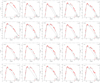 |
Fig. B.1. SED fitting of the stellar and dust emission with DUSTY for the sources in the VLBI sample. The name of each source is given in the upper left corner of each panel, and the derived luminosity is given in the upper right corner, in solar luminosity. |
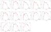 |
Fig. B.2. SED fitting of the stellar and dust emission with DUSTY for the sources in the VLBI sample. The name of each source is given in the upper left corner of each panel, and the derived luminosity is given in the upper right corner, in solar luminosity. The last two rows correspond to the outliers that were excluded from the PL relation determination (see text). |
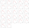 |
Fig. B.3. SED fitting of the stellar and dust emission of the C-type Miras in the DEATHSTAR sample with DUSTY. The name of each source is given in the upper left corner of each panel, and the derived distance is given in the upper right corner, in pc. |
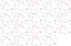 |
Fig. B.4. SED fitting of the stellar and dust emission of the S-type Miras in the DEATHSTAR sample with DUSTY. The name of each source is given in the upper left corner of each panel, and the derived distance is given in the upper right corner, in pc. |
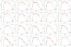 |
Fig. B.5. SED fitting of the stellar and dust emission for the M-type Miras in the DEATHSTAR sample with DUSTY. The name of each source is given in the upper left corner of each panel, and the derived distance is given in the upper right corner, in pc. |
For the carbon stars, the dust grains were assumed to be amorphous carbons with optical properties derived by Rouleau & Martin (1991). We used the COMARCS7 model atmospheres (Aringer et al. 2019) for the stellar spectra of the carbon stars, with temperatures between 2500 and 3300 K, and the same log g and microturbulence as the MARCS models. The type of dust and input stellar spectra of the S-type stars were either similar to the C- or the M-type stars, depending on their spectral class or colour, as in Ramstedt et al. (2006). A large grid of radiative transfer models with varying temperature, with steps of 100 K (T⋆ = 2400 − 3600 K and 2500−3300 K for the oxygen- and carbon-rich models, respectively); dust temperature at the inner radius of the dust shell, Td, ranging from 600 to 1200 K for the oxygen-rich models, and up to 1300 K for the carbon-rich models, with steps of 100 K; and dust optical depth at 10 μm (τ10 = 0.01 − 5.00, with steps of 0.01) was constructed. We made use of the scaling properties of the dust radiative transfer in a spherically symmetric envelope to determine either the luminosity, knowing the distance, or the other way around. We used the former to derive a new PL relation with the VLBI sources using their distances obtained from maser parallaxes (Sect. 5). The latter was used to determine the distances of the sources whose Gaia DR3 distances are not reliable or for direct comparison with the Gaia distances (Sect. 6).
For each star, the DUSTY input parameters, which are T⋆, Td, and τ10, and the bolometric stellar luminosity, L⋆, or the distance, r, were constrained by photometric flux densities collected from various online catalogues. The data consist of G, GBP, and GRP fluxes from Gaia DR3; J-, H-, and Ks-band fluxes from 2MASS (quality flag rd_flg between 1 and 3); 3.5 and 4.9 μm fluxes (L and M bands, respectively) from DIRBE; 12, 25, 60, 100 μm fluxes from the IRAS point source catalogue (quality flag 3), and fluxes at 8.6 up to 160 μm from Akari (quality flag 3) collected from the ViZier photometry viewer8 online tool. We did not include WISE data as AGB stars are known to saturate the WISE photometric instruments, in particular in the W1 and W2 bands, requiring additional calibrations to correct for residual biases (Lian et al. 2014). The fluxes were corrected for interstellar extinction using the visual extinction coefficient, AV, given by Eq. (8) in Groenewegen et al. (1992). The Aλ/AV ratios were taken from Schlegel et al. (1998) and interpolated for the relevant wavelengths. Extinction beyond 3.5 μm was neglected.
Ramstedt et al. (2008) assessed the effect of variability on the flux using several measurements from different epochs. Their results show that the variability of the star, which is particularly important at short wavelengths, can be accounted for in the uncertainty assumed for each flux point. Uncertainties of 60%, 50%, and 40% were assigned to fluxes in the J, H, and K bands, respectively. For the L and M bands, a flux uncertainty of 30% was assumed. The properties of variability at longer wavelengths are less clear due to scarce data. A 20 % calibration uncertainty was assigned to flux points beyond 5 μm. The Gaia bands were not covered in Ramstedt et al. (2008). As the amplitude of the variation is the largest at short wavelengths, we assumed an uncertainty of 75% for the fluxes measured at the three Gaia bands.
The model grid SEDs were scaled according to the median distance, rmedian, derived using the VLBI parallax and the AGB prior (or the luminosity derived with our new PL relation) until a satisfactory fit to the observational data was obtained. The best-fit to the DUSTY input parameters (see Fig. B.1) was found using the same χ2-minimization strategy as in Ramstedt et al. (2009), for example. Thereby, T⋆, Td, τ10, and L⋆ (or r) were estimated for each source. As the derived VLBI distance (or the luminosity calculated using the PL relation derived in Sect. 5) follows a distribution centred on rmedian ( ) with known lower and upper limits, we checked whether the best fit model significantly changed for the extreme distances (luminosities). We then optimised the flux scaling with the now-known T⋆, Td, and τ10 parameters. We created a posterior distribution on the luminosity L⋆ (distance r) by applying the weighted bootstrap statistical method which consists of randomly selecting a distance (luminosity) from the weighted distance (luminosity) distribution and fitting it to a sub-sample of the observed photometric data selected at random. This process was repeated 4 000 times, which allowed us to derive a median luminosity,
  (distance, rmedian), along with the 16 and 84 percentiles of the generated luminosity (distance) distribution as its confidence interval. The derived parameters are listed in Tables 3 and B.1.
The SEDs of a number of the sources that we modelled were poorly fitted. This is particularly obvious for HU Pup, QX Pup, and UX Cyg in the VLBI sample. The poor fit of QX Pup could be explained by its complex transition nature. As previously mentioned, QX Pup is classified as an OH/IR star. It is the central star of the bipolar nebula OH231.8, and is part of a system with a binary companion and a rotating circumbinary disk (Sánchez Contreras et al. 2022). The poor fit of UX Cyg could be due to its unusually turbulent envelope (Etoka et al. 2018). There is no record of signs of irregularities for the SRa variable HU Pup in the literature. For sources such as S Ser and NSV 17351, the data points were not properly fitted in the long wavelength part of the SED. In fact, the SED of a few sources exhibit a second bump at longer wavelengths (e.g. NSV 17351, GI Lup, RT Sco, TT Cen), which is usually observed in sources with a detached shell. For such sources, the SED is usually fitted with two black bodies, which was not attempted in this paper.
B.1. Comparison between black body and model atmosphere
We compared the results of the SED fitting when using a black body as stellar radiation input with the results obtained with model atmospheres. We found that the results between the two methods differ the most for oxygen-rich stars due to the strong TiO absorption in their spectra at short wavelengths. Overall, the luminosity is lower by about 25% with the MARCS models compared to with a black body. When using model atmospheres, the dust condensation temperature is systematically lower than what one obtains with a black body, by up to 35%, while the corresponding effective temperatures tend to be higher, by up to 30%, for oxygen-rich stars. The optical depths at 10 μm obtained with the two methods are in good agreement in the low-τ10 regime (τ10 < 0.8). Above that, the optical depths derived using model atmospheres tend to be smaller.
Appendix C: New distance catalogue
Best distance estimates for the DEATHSTAR sample.
All Tables
DUSTY results for the Miras in the DEATHSTAR sample for which distances were derived using our new PL relation.
All Figures
|
Fig. 1. Position of the stars in our sample. The circles represent the stars part of the DEATHSTAR sample while the red stars show the AGB stars in the VLBI sample. |
| In the text | |
|
Fig. 2. Dependence of the standard noise, the astrometric excess noise, and the RUWE of the Gaia DR3 parallax on the G magnitude and the colour GBP − GRP for the sources in the VLBI sample. |
| In the text | |
|
Fig. 3. Dependence of the standard noise, the astrometric excess noise, and the RUWE of the Gaia DR3 parallax on the G magnitude and the colour GBP − GRP for the sources in the DEATHSTAR sample. |
| In the text | |
|
Fig. 4. Comparison between the VLBI and Gaia DR3 parallaxes. The solid line represents the 1-to-1 relation. |
| In the text | |
|
Fig. 5. Gaussian fittings of the parallax difference distribution Δω/σϖ, tot for the three G magnitude categories. The distributions were normalised by the quadratically summed errors of the VLBI error with either: the DR3 parallax standard error without any correction ( |
| In the text | |
|
Fig. 6. Comparison between the astrometric excess noise of Gaia DR2 and DR3 for the VLBI sample (top) and the DEATHSTAR sample (bottom). The solid lines show the 1-to-1 relation. |
| In the text | |
|
Fig. 7. Gaia DR3 and VLBI parallaxes with the corresponding distances for the VLBI sample. Top panels: fractional errors of the VLBI (black full triangles) and Gaia DR3 parallaxes using the standard nominal error (blue open diamond) and with the corrected errors (red full circles) for the VLBI sources. The plot in the middle is a zoomed version of the plot on its left. The plot on the right compares the distances derived with Gaia DR3 parallaxes with the corrected (red) and the standard errors (blue). Bottom panels: distances derived using the four priors for the VLBI sources using the VLBI parallaxes (left) and the corrected Gaia DR3 parallaxes (middle). The solid lines represent the 1-to-1 relation. The plot at the bottom-right shows the fractional error on the derived distances. |
| In the text | |
|
Fig. 8. Gaia DR3 parallaxes and the corresponding distances for the DEATHSTAR sample. Top panels: fractional errors of the Gaia DR3 parallaxes using the standard nominal error (blue open diamond) and with the corrected errors (red full circles) for the DEATHSTAR sources. The right plot compares the distances derived with Gaia DR3 parallaxes with the corrected (red) and the standard errors (blue). Bottom panels: distances derived with the four priors for the DEATHSTAR sources using the corrected Gaia DR3 parallaxes. The solid lines represent the 1-to-1 relation. The plot on the right shows the fractional error on the corrected Gaia DR3 distances. |
| In the text | |
|
Fig. 9. Derived PL relation for Mira variables. Top: bolometric PL relation based on the luminosity of the Mira variables in the VLBI sample. The red solid line shows the PL relation obtained when using a fixed slope, and the blue dashed line represents the relation obtained when the slope is a free parameter. The sources excluded from the fit are represented by the open symbols. Bottom: comparison between our PL relation with the bolometric PL relations for C-type stars by Feast et al. (2006) in the Milky Way (F06 MW), Whitelock et al. (2006) (W06 LMC), and Whitelock et al. (2009) (W09 LMC) in the LMC. |
| In the text | |
|
Fig. 10. Comparison between the ‘good’ Gaia DR3 distances (see text) and the PL distances for the same sources. The black line shows the 1-to-1 relation. The blue and orange regions show the range of ±25 and ±50%, respectively. |
| In the text | |
|
Fig. 11. Comparison with the NESS luminosity distance. Top: the NESS luminosity distance (L) compared with the distances calculated with the various methods used in this work. The black line shows the 1-to-1 relation. Bottom: the distance fractional errors obtained in this work and those derived with the NESS luminosity distance. |
| In the text | |
|
Fig. 12. Assessment of the RUWE criterion. Top: distribution of the RUWE of the sources in the DEATHSTAR sample for the ‘good’ (blue) and ‘bad’ (red) derived Gaia DR3 distances. Middle: RUWE of the sources in the DEATHSTAR sample as a function of G magnitude, where the blue open circles and the red full circles represent distances with fractional error within and above 25%, respectively. Bottom: RUWE of the sources in the DEATHSTAR sample as a function of colour. The symbols are the same as above. |
| In the text | |
|
Fig. B.1. SED fitting of the stellar and dust emission with DUSTY for the sources in the VLBI sample. The name of each source is given in the upper left corner of each panel, and the derived luminosity is given in the upper right corner, in solar luminosity. |
| In the text | |
|
Fig. B.2. SED fitting of the stellar and dust emission with DUSTY for the sources in the VLBI sample. The name of each source is given in the upper left corner of each panel, and the derived luminosity is given in the upper right corner, in solar luminosity. The last two rows correspond to the outliers that were excluded from the PL relation determination (see text). |
| In the text | |
|
Fig. B.3. SED fitting of the stellar and dust emission of the C-type Miras in the DEATHSTAR sample with DUSTY. The name of each source is given in the upper left corner of each panel, and the derived distance is given in the upper right corner, in pc. |
| In the text | |
|
Fig. B.4. SED fitting of the stellar and dust emission of the S-type Miras in the DEATHSTAR sample with DUSTY. The name of each source is given in the upper left corner of each panel, and the derived distance is given in the upper right corner, in pc. |
| In the text | |
|
Fig. B.5. SED fitting of the stellar and dust emission for the M-type Miras in the DEATHSTAR sample with DUSTY. The name of each source is given in the upper left corner of each panel, and the derived distance is given in the upper right corner, in pc. |
| In the text | |
Current usage metrics show cumulative count of Article Views (full-text article views including HTML views, PDF and ePub downloads, according to the available data) and Abstracts Views on Vision4Press platform.
Data correspond to usage on the plateform after 2015. The current usage metrics is available 48-96 hours after online publication and is updated daily on week days.
Initial download of the metrics may take a while.