| Issue |
A&A
Volume 664, August 2022
|
|
|---|---|---|
| Article Number | A69 | |
| Number of page(s) | 13 | |
| Section | Planets and planetary systems | |
| DOI | https://doi.org/10.1051/0004-6361/202243628 | |
| Published online | 09 August 2022 | |
Discovery of an asteroid family linked to (22) Kalliope and its moon Linus★
1
Charles University, Faculty of Mathematics and Physics, Institute of Astronomy,
V Holešovičkách 2,
18000
Prague, Czech Republic
e-mail: mira@sirrah.troja.mff.cuni.cz
2
Aix Marseille Univ, CNRS, LAM, Laboratoire d’Astrophysique de Marseille,
Marseille, France
3
University of Bern, Physics Institute, NCCR PlanetS,
Gesellschaftsstrasse 6,
3012
Bern, Switzerland
Received:
24
March
2022
Accepted:
10
May
2022
Aims. According to adaptive-optics observations, (22) Kalliope is a 150-km-wide, dense, and differentiated body. Here, we interpret (22) Kalliope in the context of the bodies in its surroundings. While there is a known moon, Linus, with a 5:1 size ratio, no family has been reported in the literature, which is in contradiction with the existence of the moon.
Methods. Using the hierarchical clustering method along with physical data, we identified the Kalliope family. It had previously been associated with (7481) San Marcello. We then used various models (N-body, Monte Carlo, and SPH) of its orbital and collisional evolution, including the breakup of the parent body, to estimate the dynamical age of the family and address its link to Linus.
Results. The best-fit age is (900 ± 100) Myr according to our collisional model; this is in agreement with the position of (22) Kalliope, which was modified by chaotic diffusion due to 4–1–1 three-body resonance with Jupiter and Saturn. It seems possible that Linus and the Kalliope family were created at the same time, although our SPH simulations show a variety of outcomes for both satellite size and the family size-frequency distribution. The shape of (22) Kalliope itself was most likely affected by the gravitational re-accumulation of ‘streams’, which creates the characteristic hills observed on its surface. If the body was differentiated, its internal structure is most likely asymmetric.
Key words: minor planets / asteroids: individual: (22) Kalliope / planets and satellites: individual: Linus / celestial mechanics methods: numerical
Movies associated to Fig. 6 are available at https://www.aanda.org
© M. Brož et al. 2022
 Open Access article, published by EDP Sciences, under the terms of the Creative Commons Attribution License (https://creativecommons.org/licenses/by/4.0), which permits unrestricted use, distribution, and reproduction in any medium, provided the original work is properly cited.
This article is published in open access under the Subscribe-to-Open model. Subscribe to A&A to support open access publication.
1 Introduction
(22) Kalliope is the second largest M-type asteroid in the main belt, after (16) Psyche, and as such, it has been a promising target for spatially resolved observations (Sokova et al. 2014; Drummond et al. 2021). Recent VLT/SPHERE adaptive-optics observations of Kalliope by Ferrais et al. (2022), along with archival astrometry and interferometry of its moon Linus, led to precise estimates of its fundamental physical properties (size, shape, volume, mass, and density). Its exceptional density (≥4 g cm−3), the highest found so far among asteroids (Vernazza et al. 2021), in tandem with its low radar albedo (0.18 ± 0.05; Shepard et al. 2015), corresponding to a metal-poor (silicate-rich) surface, strongly suggests a differentiated interior. Regarding the nature of the silicates present at the surface, near-infrared spectroscopic observations suggest that these may comprise low-calcium pyroxene and possibly hydrated silicates (Hardersen et al. 2011; Usui et al. 2019). Overall, Kalliope’s case may be similar to that of Mercury, for which the high density is explained by a giant collision and mantle stripping (Asphaug & Reufer 2014), although alternative explanations exist (e.g. Brož et al. 2021).
The Kalliope−Linus binary system is also exceptional, especially because Linus is by far the largest asteroid moon (Descamps et al. 2008), possessing a diameter of (28 ± 2) km and a primary/secondary ratio of approximately 5:1. In this sense, it is similar to the Earth–Moon system (cf. 4:1). According to the accepted rule, ‘every giant moon requires a giant impact’ (Hartmann & Davis 1975; Durda et al. 2004). For asteroids located on stable orbits within the main belt, this inevitably implies that ‘every giant moon requires an asteroid family’ because fragments ejected during breakup often land on stable orbits. This was our motivation to search for the then unknown family in the vicinity of (22) Kalliope.
2 Observed Kalliope family
(22) Kalliope (osculating a = 2.909 au, e = 0.098, I = 13.701°) is located in the so called ‘pristine zone’ (Brož et al. 2013) of the main belt, which is surrounded by strong mean-motion resonances with Jupiter, namely by the 5:2 resonance at 2.82au and the 7:3 resonance at 2.96 au. Consequently, it is strongly depleted because small, kilometre-sized asteroids drifting via the Yarkovsky effect have relatively short lifetimes, compared to the middle and outer belts.
We used recent catalogues of proper elements (Knezevic & Milani 2003; Radovic et al. 2017; Novakovic & Radovic 2019) and of albedos (Nugent et al. 2015; Usui et al. 2011) to plot Fig. 1. One can immediately identify a number of known families (Nesvorný et al. 2015), including the one denoted (7481) San Marcello, which is surprisingly close to (22) Kalliope. For reference, its family identification number (FIN) is 626.
Moreover, we realised that the semi-major axis of (22) Kalliope coincides with the three-body resonance 4–4–1 with Jupiter and Saturn at 2.91 au (Nesvorný & Morbidelli 1998), and it is shifted in eccentricity by 0.01 with respect to the family FIN 626 (cf. Fig. 2). This is most likely due to chaotic diffusion (see the confirmation in Sect. 4). In this work, we thus suggest that the whole 626 family is associated with (22) Kalliope (the FIN always remains the same).
We used the hierarchical clustering method (HCM; Zappalà et al. 1995) to extract the family. However, our initial body was still (7481), not (22), because it is too separated. The maximum possible cutoff velocity was υcut = 75 m s−1; (22) was added ‘manually’. Interlopers were removed automatically if they did not fulfil our criteria for members: visible albedo pV ∈ (0.1; 0.35) and colour index a★ ∈ (−0.5; 0.025) mag. The result is shown in Fig. 2. The overall extent roughly corresponds to the escape speed from the parent body (i.e. υesc = 116 m s−1). The Kalliope family exhibits a typical ‘V-shape’ (Vokrouhlický et al. 2006), with the centre ac = 2.9095 au and the parameter C = 1.5 × 10⁻⁴. (22) Kalliope is located close to this centre because a semi-major axis is not changed by chaotic diffusion in a mean-motion resonance. Given the median albedo pV = 0.195 and the bulk density ρ = 4.1 g cm−3 (according to the shape derived by the Viikinkoski et al. 2015 method), the upper limit for the age is (Nesvorný et al. 2015)
 (1)
(1)
A larger dispersion in eccentricity (0.03 vs. 0.01) is observed on the left-hand side of the 17:7 mean-motion resonance with Jupiter, presumably due to the Yarkovsky drift across the resonance. Consequently, the majority of family members were originally located on the right-hand side.
The size-frequency distribution (SFD) was computed from 302 members. It exhibits a steep part (slope −3.0) and a very shallow part (−1.5) below D < 5 km (Fig. 3), which is typical for dynamically depleted populations.
A preliminary comparison to a set of smoothed particle hydrodynamics (SPH) simulations (Durda et al. 2007) indicates a parent body size of Dpb = (157 ± 2) km, a projectile size of d = (29 ± 10) km, a largest remnant (LR) mass ratio of Mlr/Mpb = 0.92 ± 0.05, a largest fragment (LF) of Mlf/Mpb = 0.00036 ± 0.00010, and a specific energy of Q/Q★ = 0.10 ± 0.05, where Q★ corresponds to the scaling law of Benz & Asphaug (1999). Because the outcome depends on so many parameters, including the impact speed, υ, and the impact angle, ϕ, the solution is not unique and alternative fits of the SFD are possible. Nevertheless, a re-accumulative event is expected at the origin of the Kalliope family. This is closely related to the observed shape of (22) Kalliope, which is aspherical (Fig. 7), similar to other M-type bodies. Material rheology and non-zero friction during re-accumulation must support all these topographic features.
According to Durda et al. (2004), Linus may be classified as a smashed-target satellite. If we also include it in the SFD, the collision should be even more energetic. Actually, Linus appears as an intermediate-sized fragment, and its volume represents about twenty 10-km bodies. It may thus be difficult to explain the existence of Linus and the remaining fragments at the same time.
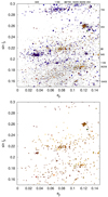 |
Fig. 1 Observed proper eccentricity (ep) vs. sine of proper inclination (sin Ip) of bodies in the ‘pristine zone’, with the proper semi-major axis ap ∊ (2.82; 2.96) au. All bodies are plotted in the top panel, and a subset of bodies with a geometric albedo pV ∊ (0.1; 0.35) according to the WISE catalogue (Nugent et al. 2015) are plotted in the bottom panel. Colours correspond to pV (blue → yellow). If pV is unknown, the colour is grey. The high-albedo family previously designated as (7481) San Marcello = FIN 626 is now associated with (22) Kalliope (bold number). Numerous known families are indicated (numbers at the border), namely (293), (709), (845), (1189), (18405), and (36256). |
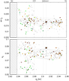 |
Fig. 2 Observed Kalliope family in the space of proper elements ap, ep (bottom) and sin Ip (top). It was identified via the hierarchical clustering, for the cutoff velocity υcut = 75 m s−1. Interlopers are indicated by green circles. The mean-motion resonances 5:2, 17:7, 12:5, 4–4–1, and 7:3 are plotted with dotted lines. The extent of the 5:2 resonance is shown as the hatched area. (22) Kalliope is located in the three-body resonance 4–4–1 with Jupiter and Saturn, which explains why it is separated from the family. The iso-velocity ellipses were computed for the escape velocity υesc = 116 m s−1 and specific values of the true anomaly and the argument of pericentre: f = 90°, 100°, 110°, ω + f = 60°, 70°, 80°. |
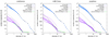 |
Fig. 3 Collisional evolution of the main belt (blue) and the Kalliope family (pink). Cumulative size-frequency distributions N(>D) are plotted. The observed main belt population is taken from Bottke et al. (2015) and the observed Kalliope family from this work (green). We assumed three different initial conditions (black dashed): a continuous size-frequency distribution (left), with Linus and depleted D > 10 km bodies (middle), and a populous distribution (right). Each simulation was run ten times (multiple pink lines) in order to account for the stochasticity of collisions. The respective best-fit ages are 800 Myr, 900 Myr, and up to 3.4 Gyr. |
3 Collisional evolution
We simulated the long-term collisional evolution with the Boulder code (Morbidelli et al. 2009). The collisional probabilities and impact velocities for the relevant populations – main belt (MB) and the Kalliope family – were computed as follows:
The scaling law is similar to that in Benz & Asphaug (1999), with a lower strength at D ≃ 100 m in order to match the observed SFD of the main belt, namely
 (2)
(2)
where Q0 = 9 × 10⁷ erg g−1, a = −0.53, B = 0.5 erg cm−3, b = 1.36, and R = D/2 (in cm). For simplicity, we also assumed the same density, ρ = 4.1 g cm−3, as for (22) Kalliope (for the ADAM shape model; Ferrais et al. 2022), but if it is differentiated, it may be more logical to assume a lower density for fragments, corresponding to silicates (ρ ≃ 3 g cm−3). On the other hand, for (22) itself, the value of Q might be larger than nominal if it is differentiated.
We accounted for a size-dependent dynamical decay, as described in Cibulková et al. (2014). The decay in the pristine zone is relatively fast, given the distance between the 5:2 and 7:3 resonances (0.14 au). Compared to the inner main belt (0.4 au), we expect it to be about three to five times faster. For Linus, we artificially increased its lifetime, as it is bound to (22) Kalliope. Because the family itself must have been extended even at t = 0, some bodies were initially close to or inside the resonances (as in Sect. 4).
Initial conditions for the main belt were close to the observed SFD because it is close to a steady state. On contrary, we assumed a steep SFD for the synthetic family, even below D < 5 km, because there is no apparent reason why it should be so shallow. Moreover, there is another source of material we should not forget – the 28-km-wide Linus, which is a regular intermediate-sized family member. We included Linus in the SFD because secondary collisions with Linus may contribute to the SFD.
Our results are plotted in Fig. 3. Each simulation was run ten times in order to account for the stochasticity of collisions. If the initial conditions correspond to a smooth power law with the slope q = −3.0, it is impossible to explain the break at 5 km as well as the non-existence of D > 10 km bodies. To fit both features, the SFD must be initially without D > 10 km bodies, which actually creates the break at 5 km in the course of colli-sional evolution (Fig. 3, middle). The minimum age of the family is then 800 Myr.
Alternatively, if the initial SFD is scaled up by a factor of 5, with an extremely steep slope, q = −10, at the large-size end and a shallow slope afterwards, the whole SFD simply evolves downwards and ends up similar as before; the age may reach up to 3.4Gyr. However, it is unlikely that the family is so old, because its initial SFD is so extreme. In 10% of such simulations, Linus experienced a catastrophic collision, which would be in contradiction with its very existence.
| MB–MB | 2.86 × 10⁻¹⁸ km−2 yr−1 | 5.77 km s−1 |
| MB–Kalliope | 3.17 | 5.58 |
| Kalliope–Kalliope | 5.80 | 4.75. |
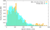 |
Fig. 4 Histogram of the ejection speed in our orbital model (blue), compared with one SPH simulation from Sect. 5: l75_45_6_0 (orange). The escape speed is indicated by the dotted line. |
4 Orbital evolution
We simulated the long-term orbital evolution with the numerical integrator SWIFT (Levison & Duncan 1994), supplemented with the Yarkovsky effect, the Yarkovsky-O’Keefe-Radzievskii-Paddack (YORP) effect, collisional reorientations, or mass shedding (Brož et al. 2011).
Our synthetic Kalliope family was created as an artificial breakup with an assumed velocity field. It contains ten times more bodies than the observed SFD in order to have enough kilometre-sized bodies at late stages. The velocity distribution is size-dependent, with υx(D) = 24 m s−1 (D/5 km)−1, as are the other components. The histogram of |υ| exhibits a characteristic peak at the escape velocity, and this is similar to the outcomes of SPH simulations (see Fig. 4 and Sect. 5). The field is isotropic in the Cartesian space. Of course, in the osculating element space, the distribution is no longer isotropic – it is instead given by the impact geometry, namely the true anomaly, f = 100°, and the argument of pericentre, ω = 330°, so iso-velocity ellipses resemble the core of the family (as in Fig. 2).
The time step was Δt = 36.525 d and the time span t2 − t1 = 1 Gyr. Mean elements were computed using convolution filters (Quinn et al. 1991), with the input sampling 1 yr, filters A, A, A, B, decimation factors 10, 10, 10, 3, and the output sampling 3000 yr. Proper elements were determined by the frequency-modified Fourier transform (Šidlichovský & Nesvorný 1996) from 1024 samples, and the output sampling was 0.1 Myr. This output is mostly compatible with other types of proper elements; a minor difference was apparent for proper inclinations below ap = 2.88 au. An artefact (sin Ip lower by 0.02 in Fig. 5) may occur if the ɡ or s frequencies of orbits approaching the 5:2 resonance become too close to the passbands of our digital filters. A solution would be to use a modified setup (e.g. A, A, B, B); nevertheless, other parts of the proper elements space were not affected.
Our results are plotted in Fig. 5. Initially, the synthetic family extended across the pristine zone along the semi-major axis due to outliers in the velocity field. On the contrary, it was narrow in eccentricity and inclination, as was the core of the observed family. (22) Kalliope and all its clones were located in the 4–1–1 resonance.
In the course of evolution, the number of bodies decreases due to the Yarkovsky drift, perturbations by the 5:2 and 7:3 resonances, and scattering by Jupiter; the exponential decay timescale, τ, is approximately 1.2 Gyr. The synthetic family becomes more spread not only in a, but also in e, I due to the 17:7, 12:5, and 4–1–1 resonances. Interestingly, (22) Kalliope and its clones chaotically diffuse, which offers an opportunity to determine the age independently. For the time t ≲ 500 Myr, the number of bodies below the 17:7 resonance and their spread is insufficient. For the time t ≳ 1 Gyr, the majority of (22) clones are spread by more than 0.01 in e. Taken together, the age of the family must be (750 ± 250) Myr. This is fully compatible with the collisional evolution (Fig. 3, middle). In fact, it also confirms that a hypothesis of a 3.4 Gyr old family (Fig. 3, right) is excluded. A more precise age determination is not possible due to the limited number of observed bodies and the systematic uncertainty of the density of ejected fragments. This is closely related to the internal structure of the parent body.
5 SPH simulations
We simulated a breakup of the Kalliope parent body by means of the SPH, with the Opensph solver (Ševeček et al. 2019; Ševeček 2019). A principal question is whether differentiated is different from homogeneous. Of course, the body has a certain density profile, ρ(r) (cf. Ferrais et al. 2022), but hereinafter we are interested in the ρ of the ejecta, or in the chemical composition (silicates vs. metal). According to an analogy with the Earth-Moon system, we would expect the moon to have a lower ρ, corresponding to the mantle, not to the core (Canup 2014). The same is true for other ejecta.
Another principal question is how much ejecta must be ejected (to ∞) in order to form a massive moon on a bound orbit (to ≪ ∞), in other words, whether the observed Kalliope family is compatible with Linus.
Initial conditions of our simulation are somewhat simplified. We assumed the target is either spherical or a Maclaurin ellipsoid (i.e. either static or rotating). The interior was differentiated, composed of a metallic core (8 g cm−3) and a silicate mantle (3 g cm−3), or alternatively, homogeneous (for comparison). Depending on the structure, we expected substantial differences in shock wave propagation, reflection, attenuation, focussing, ejection of material, and so on. The spherical target diameter D = 153 km, and the projectile diameter, d, was varied. The core-mantle boundary was adjusted so that the total mass and volume correspond to the observed values (Ferrais et al. 2022); the core diameter was then Dc = 92 km. We expected that low- and mid-energy collisions would not eject too much mass. High-energy collisions may require a somewhat larger target. Moreover, they may potentially explain a high density of the remnant if enough mantle material is ejected. The initial specific internal energy was low (103 J kg−1) and constant throughout the interior. The targets were put in hydrostatic equilibrium before impact.
Similar computations were made for Maclaurin ellipsoids. We assumed the current rotation period, P = 4.1482 h, and estimated the eccentricity from (ω = 2π/P)
 (3)
(3)
Therefore, the core is less eccentric than the mantle.
We also varied the impact velocity, υimp, between 5 and 6km s−1 and the impact angle, ∅imp, from 0 to 45°. In the case of ellipsoids, the impacts were in the equatorial plane. Materials were described by the Tillotson (1962) equation of state, Drucker–Prager rheology, Grady–Kipp fragmentation, and Weibull flaw distribution, where principal parameters were taken from Benz & Asphaug (1999); Maurel et al. (2020) and are listed in Table 1. The yield strength was dependent on the internal energy. The core material is modelled with the same strength model as the mantle (but with different constants).
We solved the hydrodynamic equations for the three phases: stabilisation (100 s), fragmentation (10000 s), and re-accumulation (300000 s). In the first and second phases, we used an asymmetric SPH solver and adaptive smoothing lengths, but the maximum smoothing length, h, was set to 17 500 m, or 5.1 times the initial h, to prevent excessive CPU time due to expanded particles at the core-mantle boundary; we also used the rotation correction tensor, a hash map for nearest neighbours, artificial viscosity, self-gravity, the opening angle 0.5, and the multipole order 3 (Ševeček 2021). In the third phase, we started with an equal-volume handoff and continued with a simplified N-body solver, merge-or-bounce collision handler, repel-or-merge overlap handler, the normal restitution 0.5, the tangential restitution 1, the merge velocity limit 4 (see explanation in Ševeček 2021, p. 120), and the merge rotation limit 1. The total number of particles was 105.
Before proceeding further, we recall the basic parameters of the Earth-Moon-forming impact for comparison. According to Canup (2014), it occurred with the impact speed υimp/υesc < 1.1, the impact parameter b ≃ 0.7, and the projectile mass fraction γ ≃ 0.125. The Moon accreted from a circumplanetary disk. In this scenario, the disk mass is high if υimp ↓, b ↑, γ ↑, the disk mass is low if υimp ↑, and it is variable if b < 0.7.
In the case of (22) Kalliope, the relative speed, when normalised by υesc, is orders of magnitude higher, υimp/υesc ≃ 50, that is to say, a totally different regime. The projectile angular momentum for an intermediate angle was of the order of Limp = 2 × 1025 kg m2 s−1 = 1.9 Lrot, which is comparable to the current rotational angular momentum of (22) Kalliope. However, in the re-accumulative regime (Vernazza et al. 2020) one can hardly expect angular momentum embedding; draining, when the impact ejects material from an already rotating target, is more likely (Ševeĉek et al. 2019).
Our results are summarised in Fig. 6. The impacts actually span a range of energies, from low energy, which did not eject enough fragments (i.e. it ‘undershot’ the SFD), to high energy, which ejected ten times more (‘overshoot’). This was needed to understand overall trends. At the same time, we monitored the shape of the LR (i.e. (22) Kalliope); the respective changes were from minor to major, which is to be expected in the re-accumulative regime.
Low-energy impacts. In the case of low-energy, spherical, 45° impacts (Fig. 6, Cols. 1 and 2), the SFD is undershot; the LF is only 5 km, but the observed LF is 10 km. While this is clearly a poor fit, it is important to note the shape of the LR. We can monitor it until the end of the fragmentation phase; it is determined by two general processes: (i) ejection of material from around the antipode, which falls back to the surface on a short timescale, but not back to the antipode because the LR has started to rotate due to the AM draining; and (ii) excavation at the impact point, with material flying on ballistic trajectories, which falls back in the Keplerian time on the other hemisphere, which again has rotated in the meantime. This creates two characteristic ‘hills’ on the surface (see the animations associated with Fig. 6). Interestingly, it is very similar to the two hills in the −ŷ direction observed at the surface of (22) Kalliope (Fig. 7). We thus cannot exclude the possibility that they were created late, by a low-energy impact. Because material is fully damaged, the coefficient of friction has a crucial impact on the resulting shape (as in Vernazza et al. 2020).
Another general feature is a flatter surface, perpendicular to the impact direction, created by excavation. It is similar to the observed shape in the +ŷ direction. The overall shape remains too close to spherical, though; medium energy would be needed at the least.
If the interior is differentiated, the surface is even flatter because the core is denser and its moment of inertia slows down its motion. Moreover, the core after impact is no longer spherical; it is also flatter and much closer to the surface on the side of impact. This configuration is non-hydrostatic, though, and might further evolve over geologic timescales.
Medium-energy impacts. For medium-energy impacts into Maclaurin ellipsoids (Fig. 6, Cols. 3 and 4) the outcome was variable. For a homogeneous body, the SFD is overshot and contains an intermediate-size fragment (between the LR and LF in size). We believe it should be possible to find a better solution for the SFD, but we did not find it in our limited set of simulations. Nevertheless, the overall shape is now elongated enough, with the two peaks still present. From a broader perspective, re-accumulation takes the form of ‘streams’, with material gravitationally attracted from larger distances.
For a differentiated body, ejection is sufficient to match the LF, but not Linus. The asymmetry of the core is even more pronounced. Another difference is that the core is closer to the surface elsewhere, as in the  direction in Fig. 7. Even though we do not have enough resolution to see fine-grained ejecta, one side of the core was fully exposed in the course of impact, and we expect that metallic ejecta must partly cover the surface. This is fully compatible with the M-type taxonomy of (22) Kalliope.
High-energy impacts. Increasing energy (Fig. 6, Cols. 5 and 6) further leads to the SFD being overshot. Nevertheless, the highest energy actually produced Linus as the LF, but it is on an unbound orbit. We also do not see any disk-like structure from which a bound moon could be formed. The slope is steep from D = 30 km, and the total number of fragments is ten times larger than observed (i.e. similar to the old ‘populous’ family from Sect. 3). However, we find it difficult to eliminate 100 D > 10 km bodies from the SFD by long-term evolution to match the observed SFD. It would also be in contradiction with the chaotic diffusion of (22) Kalliope, as discussed in Sect. 4.
The LR is substantially smaller than the parent body. A homogeneous composition and a head-on impact led to splitting and a pair of unbound similarly sized LRs. This is in contradiction with observations of Kalliope, but it is a logical continuation of the trend from low- to medium- to high-energy impacts. (A small-sized version of this phenomenon was studied by Vokrouhlický et al. 2021).
For a differentiated body, the core is exposed even more because re-accumulation is not as efficient. At the same time, one may expect late secondary impacts of metallic material. Again, this is compatible with the M type.
During breakups, the final densities of the LR, the LF, and other fragments are generally different from the initial densities. Ejection of low-density mantle material is a logical explanation for the high density of (22) Kalliope. At the same time, Linus – if created during this breakup – should be composed of mantle material and have a low density, analogously to the Earth–Moon system. Unfortunately, our model does not allow us to accurately estimate the final densities for three reasons: (i) at the end of the fragmentation phase, material compression is still ongoing; (ii) during the re-accumulation phase, densities are fixed (by the handoff); and (iii) our model does not contain a treatment of porosity and compaction. What we can do in the future is to prolong our computations 30 times so that re-accumulation is also treated in the SPH framework.
Of course, we did not fully explore the parameter space, for example for high initial rotation, oblique, non-equatorial, or retrograde impacts. Fast initial rotation might help create a massive moon (Linus). Nevertheless, we think the initial rotation was not too fast (not close to critical) because the two hills would then be too separated from each other. Moreover, impacts should have some  velocity component because the hills have slightly different z coordinates.
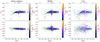 |
Fig. 5 Orbital evolution of the Kalliope family. Proper semi-major axis, ap, vs. proper eccentricity, ep (bottom) as well as proper inclination, sin Ip, are plotted in the course of time: initial conditions (left), 200 Myr (middle), and 1 Gyr (right). Colours and symbols correspond to the actual diameters. The observed family is plotted for comparison (green). The number of synthetic bodies is ten times larger (3020 vs. 302) to improve the statistics. Evolution is driven by the Yarkovsky effect and mean-motion resonances, especially 12:5 and 4–1–1; (22) Kalliope (yellow) is affected by the latter. |
Material parameters of the SPH simulations.
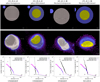 |
Fig. 6 SPH simulations and resulting size-frequency distributions of the Kalliope family: initial conditions (0 s; top), end of the fragmentation phase (10 000 s; middle), and end of the re-accumulation phase (300 000 s; bottom). We tested different initial conditions: homogeneous sphere (Col. 1), differentiated sphere (Col. 2), homogeneous Maclaurin ellipsoid (Col. 3), and differentiated Maclaurin ellipsoid (Col. 4). The title (XXX_YY_Z_ŽŽ) corresponds to the target diameter (in km), projectile diameter (km), impact speed (km s−1), and impact angle (deg). We only plot a subset of SPH particles that have |z| < 10 km to have a clear view of the interior. Their colours correspond to the density, ρ, on the scale: violet (~0), blue (2.7), white (4.1), and yellow (8 g cm−3). Animations are available online. |
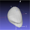 |
Fig. 7 Shape of (22) Kalliope according to the ADAM model, with two ‘hills’ approximately in the −ŷ direction, separated by approximately 15° in longitude. |
6 Discussion
6.1 Stochasticity in SPH simulations
A late phase of gravitational re-accumulation, even if it is described by a fully hydrodynamical (SPH) simulation, corresponds to a few-N-body problem because there are only a few big bodies left. Such systems are known to exhibit deterministic chaos (e.g. Nekhoroshev 1977). In our case, the very existence of Linus in our simulations, and whether it is bound or unbound, likely depends on a few collisions, which either occur or do not.
The Earth-Moon-forming impacts also exhibit a broad range of outcomes (Canup et al. 2019), and only some of them are analogous to the Earth–Moon system. Consequently, we expected more simulations would be needed (up to 102) to fit the Kalliope-Linus system (or the complete SFD). Yet, the number of free parameters to describe the respective geometry, rotation, energetics, and materials is of the order of 101. We thus postpone a computation of a corresponding ‘matrix’ of simulations to future work.
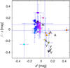 |
Fig. 8 SDSS colour indices a★ versus i − z (Parker et al. 2008) for the Kalliope family. Most correspond to C/X-complex taxonomy or to M-type taxonomy if albedo is also taken into account. A subset of bodies with known colours is plotted (circles with error bars); probable interlopers are indicated by green circles. Examples of taxonomic classes related to differentiated bodies are also indicated by letters (‘V’, ‘A’, and ‘M’); these are not family members. |
6.2 Constraining the origin of Kalliope
The Kalliope collisional family is the second known family related to a differentiated body after that of Vesta. As such, it allows the differentiation process on such an early formed body to be investigated and characterised. In our current understanding, differentiated bodies comprise mostly V types (basaltic), A types (olivine), and M types (metallic). Both spectroscopic observations of the primary and the Sloan Digital Sky Survey (SDSS; Parker et al. 2008) colours of the family members (Table B.1 and Fig. 8) imply a C/X-type classification for nearly all family members. When adding the albedo information for these objects (which possess moderate optical albedos in the [0.1; 0.35] range), it appears that essentially all family members are M-type asteroids, as is (22) Kalliope. In our search for possible A- and V-type family members, we identified six bodies that exhibit colours similar to S types (38309, 112382, 127063, 145265, 2002 OP6, and 373880), or possibly V types in one case (373880). Given that the orbital properties of most of these bodies are quite different from those of the core of the family, we consider them interlopers.
The prevailing M-type classification confirms the absence of olivine ((Mg,Fe)2SiO4), this mineral being the standard one expected for mantles of differentiated bodies. Actually, olivine-rich bodies are rare everywhere in the asteroid belt (DeMeo & Carry 2013; DeMeo et al. 2019), which led authors to suggest that the parent bodies of differentiated meteorites may have been battered to bits (Burbine et al. 1996). The formation of an olivine-rich mantle may not, however, have been the norm, especially if bodies such as Kalliope formed beyond the snow line among the later-formed carbonaceous chondrite-like bodies. As suggested by Hardersen et al. (2005), if Kalliope’s parent body initially contained as much carbon as found in carbonaceous chondrites along with iron-bearing olivine as commonly found in CO, CV, or CR chondrites, then it could have experienced a smelting-type reaction provided that it experienced internal temperatures above 850 °C. In Kalliope’s case, such a high internal temperature is expected given its differentiated interior and metal-rich core. The smelting-type reaction implies that if sufficient carbon is present as a reducing agent, the final products will be enstatite (MgSiO3), or other iron-poor pyroxene, metallic iron, and possibly silica (SiO2) (Hardersen et al. 2005).
A formation beyond the snow line for a large fraction of main-belt M-type asteroids would be consistent with the majority of these bodies residing in the outer belt (DeMeo & Carry 2013), a region essentially populated by bodies (C, P, and D types) that likely formed beyond the snow line (Vernazza et al. 2021). (22) Kalliope may, as such, be a likely parent body of carbonaceous-chondrite-related iron meteorites (Kruijer et al. 2017).
7 Conclusions
In this work, we have studied the Kalliope family. First, the family was difficult to find because it has been dispersed and because the orbit of (22) Kalliope has been changed by chaotic diffusion. As we already know, the HCM has limitations, for example, in identifying family halos (Brož & Morbidelli 2013) and recognising interlopers, or it may fail to identify the LR, (22) Kalliope. Families may be even harder to find than previously thought, especially if they are old, dispersed, and depleted by long-term orbital and collisional evolution. Nonetheless, satellites (smashed targets in particular) are good indicators of families. It independently confirms that (107) Camilla and (121) Hermione, with non-existent families but existing satellites, may have had families (Vokrouhlický et al. 2010) prior to early instabilities in the Solar System.
Second, according to our simulations, it is possible to outline a consistent scenario. The parent body broke up (900 ± 100) Myr ago due to an impact with a 29 to 45-kilometre-wide projectile. (22) Kalliope was partly preserved and partly re-accumulated; ejected material was mostly from the silicate mantle, which explains why (22) Kalliope, with a preserved iron core, has the exceptional density 4.1 g cm−3. We successfully explain the formation of hills on the surface by re-accumulation. Unfortunately, we did not find a simulation in our limited set that would produce a 1:1 counterpart of the observed moon Linus on a bound orbit, but we have ‘cornered’ a parameter space in which a solution will be found. Long-term collisional as well as orbital evolution then explains not only the very shallow SFD, but also the uneven spread in eccentricity due to the 17:7 resonance and the offset of (22) Kalliope in eccentricity due to the 4–1–1 resonance, all on the correct timescale. (See also Appendix A for a discussion of Linus’s orbit.)
Third, if the parent body were differentiated and axially symmetric, with the centre of mass coinciding with the centre of volume, after breakup the asymmetry of the internal structure would be so substantial that it would also affect the dynamics of the moon orbit. We predict that the iron core is close to the surface on one side of the body, likely the flatter side (in the +ŷ direction; Fig. 7). The surface of this M-type asteroid is unevenly covered with metallic ejecta. All these features should eventually be constrained by observations, for example spatially resolved polarimetric measurements or reflex motion with respect to a suitable reference.
Given the systematic uncertainties of densities of other fragments (family members), it would be very useful to systematically search for binaries among them. If they make up one-sixth of the binaries in the main belt, and presumably an old family evolves similarly as the main belt, we expect 50 binaries, either escaping ejecta or YORP spin-ups. Some of them should exhibit eclipses, which is an opportunity to determine the average density of components as
![$\rho = {{3\pi } \over G}{\left[ {{{\left( {{{{R_1}} \over a}} \right)}^3} + {{\left( {{{{R_2}} \over a}} \right)}^3}} \right]^{ - 1}},$](/articles/aa/full_html/2022/08/aa43628-22/aa43628-22-eq6.png) (4)
(4)
where R1, R2 denote their radii and a the semi-major axis. If the value is lower than Kalliope’s average density, it will be an independent confirmation of its differentiation because we expect binaries to originate from Kalliope’s mantle. It may be difficult if not impossible to distinguish differentiation from alternative processes, though – in particular because ejected material is expanded during the fragmentation phase, re-accumulated as a porous material, and compacted on possibly long timescales.
Movie
Movie 1 associated with Fig. 6 (kalliope) Access here
Acknowledgements
This work has been supported by the Czech Science Foundation through grant 21-11058S (M. Brož). We thank the referee A. Morbidelli for comments, which helped us to re-think implications of our work.
Appendix A Evolution of the Linus orbit
We also estimated the timescale of evolution of Linus’s orbit. For the tidal torque acting on Linus, we applied the standard formula (de Pater & Lissauer 2010):
 (A.1)
(A.1)
where Γ denotes the torque, L the orbital AM, a the semi-major axis, m2 the mass of the perturbing body (Linus), R1 the radius of the perturbed body (Kalliope), m1 its mass, k2 the Love number, and Q the dissipation factor. The free parameter is the ratio k2/Q. Unfortunately, it is unconstrained by observations. According to our tests, a model with tides (Mignard 1979; Brož et al. 2022) is statistically equal to a model without tides. Nevertheless, we can assume tides to be either strong (Q = 40, k = 0.305 as for (216) Kleopatra; Brož et al. 2022) or weak (Q = 280 as for the Earth, k = 0.024 as for Moon).
Similarly, for the radiative torque on synchronous satellites, we applied the scaling from Ćuk & Burns (2005):
 (A.2)
(A.2)
where ah denotes the heliocentric semi-major axis, ρ the density, a1 the binary semi-major axis, R2 the radius of the secondary, and P1 the binary period. The quantities with 0 subscripts are normalisations. Again, the radiative effects can be strong (the same coefficient as above) or weak (0.5 •·10−12 s−1). The sign of Γ is either positive or negative; it depends on the detailed (unknown) shape of the moon.
The comparison (Fig. A.1) shows that the two torques should be comparable between 1200 and 3000 km. Interestingly, Linus is located 1060 km from the primary, very close to an equilibrium between the weak positive tidal and strong negative radiative torques. It seems reasonable that tidal dissipation is weaker in (22) Kalliope than in (216) Kleopatra because the former is likely differentiated (more rigid, less viscous) and certainly not as extreme as the latter.
The timescale of evolution, starting from the Roche radius, corotation orbit (COR), or the last stable orbit (LSO), is about 108 y up to the location of Linus, but of course an approach to the exact equilibrium is very slow (5 • 108 y). If both torques were positive and there were no equilibrium, the overall evolution up to the 0.5 Hill radius would take 2 • 109 y. Clearly, even weak tides are sufficient to explain the evolution of Linus well within the minimum dynamical age of the Kalliope family.
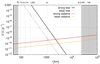 |
Fig. A.1 Expected torque per angular momentum, |Γ|/L, versus distance, r, in the Kalliope–Linus system. We separately plot the tidal (black, grey) and the radiative (red, orange) torques. We also distinguish two levels of the tidal dissipation as well as two levels of the radiative effects. Linus is located at a1 = 1060 km, i.e. close to a possible equilibrium between the torques. |
Appendix B List of family members
In the following, we list all 302 family members (with interlopers removed):
(22) Kalliope, (22) Linus, 7481, 12573, 14012, 14338, 16367, 17845, 17994, 18733, 21216, 21741, 22087, 22108, 24879, 25631, 26023, 26213, 27916, 28089, 31064, 31709, 32646, 34565, 37292, 37669, 41358, 41930, 46212, 46272, 47061, 47898, 50806, 51259, 53350, 54280, 54908, 55418, 62032, 68222, 71357, 71396, 73446, 82711, 82731, 82787, 85417, 94038, 94199, 95912, 104173, 110549, 111144, 111199, 112430, 112631, 114664, 116170, 119834, 131265, 140031, 140108, 141200, 150541, 152341, 152606, 153086, 154059, 159032, 161396, 161565, 161837, 164369, 166751, 171194, 175716, 177128, 178329, 180960, 181005, 190114, 196897, 196974, 203800, 206688, 216530, 217802, 226746, 227719, 228284, 229227, 232543, 237969, 245390, 246484, 248020, 250675, 254820, 254988, 261583, 267786, 277936, 279504, 280659, 284640, 285991, 286015, 295381, 296463, 296943, 304544, 305259, 306388, 316440, 318919, 319447, 322682, 325905, 326039, 327530, 328400, 329280, 331508, 331810, 333674, 334501, 334874, 338276, 351859, 357736, 360902, 361395, 363398, 366347, 368462, 368809, 378902, 380475, 387687, 396582, 400928, 403919, 404857, 409327, 410858, 413399, 414629, 415732, 420228, 423037, 426532, 427317, 428933, 430340, 440414, 444625, 454161, 454418, 462450, 464107, 464304, 464612, 472463, 477110, 483146, 485768, 487450, 488123, 492163, 501370, 503314, 505186, 505266, 507356, 510489, 515640, 518825, 520740, 521968, 523413, 526488, 529676, 532317, 532409, 533253, 536305, 538932, 539027, 539263, 545524, 546186, 549084, 551844, 555164, 559437, 560485, 562647, 562836, 563578, 563959, 564493, 566962, 569114, 569157, 571468, 573702, 576659, 576709, 576969, 581697, 582004, 582022, 583589, 583772, 588322, 590269, 590279, 594884, 598037, 600315, 601088, 601468, 604253, 1999 FS99, 2000 SX379, 2002 CB315, 2002 RC265, 2003 SE228, 2004 KB20, 2005 TY83, 2005 VY137, 2005 WN116, 2006 CW31, 2006 YF37, 2007 EQ145, 2007 FY54, 2007 RU52, 2007 TX459, 2007 VN347, 2007 VX305, 2008 EW42, 2008 JF12, 2008 KB45, 2008 SM319, 2008 TC197, 2008 UH232, 2009 SA113, 2010 FU140, 2010 RS77, 2010 TT192, 2010 YY3, 2011 CW125, 2011 EX91, 2011 FR66, 2011 UO420, 2012 BG62, 2012 GG42, 2012 UY194, 2012 XM102, 2013 HS125, 2013 VA36, 2014 EG244, 2014 HH165, 2014 MO66, 2014 NZ22, 2014 QH248, 2014 QN72, 2014 QV508, 2014 QX473, 2014 QZ103, 2014 RL31, 2014 SV118, 2014 WO214, 2014 XX3, 2015 BR379, 2015 DH253, 2015 DO258, 2015 FH411, 2015 GZ21, 2015 HG4, 2015 KB83, 2015 KD83, 2015 MP57, 2015 MZ90, 2015 SQ24, 2015 TH272, 2015 UH30, 2015 VU85, 2015 VZ37, 2015 XB413, 2015 XG358, 2015 XQ277, 2016 AO141, 2016 CP87, 2016 EL258, 2016 KT10, 2016 QV66, 2016 UF8, 2017 BD122, 2017 SM30, 2017 UJ49, 2018 LS17, 2018 OK1.
Compilation of known albedos and taxonomic types of the Kalliope family members.
References
- Asphaug, E., & Reufer, A. 2014, Nat. Geosci., 7, 564 [NASA ADS] [CrossRef] [Google Scholar]
- Benz, W., & Asphaug, E. 1999, Icarus, 142, 5 [NASA ADS] [CrossRef] [Google Scholar]
- Bottke, W. F., Brož, M., O'Brien, D. P., et al. 2015, The Collisional Evolution of the Main Asteroid Belt, (Tucson: University of Arizona Press) 701 [Google Scholar]
- Brož, M., & Morbidelli, A. 2013, Icarus, 223, 844 [CrossRef] [Google Scholar]
- Brož, M., Vokrouhlický, D., Morbidelli, A., Nesvorny, D., & Bottke, W. F. 2011, MNRAS, 414, 2716 [CrossRef] [Google Scholar]
- Brož, M., Morbidelli, A., Bottke, W. F., et al. 2013, A&A, 551, A117 [Google Scholar]
- Brož, M., Chrenko, O., Nesvorny, D., & Dauphas, N. 2021, Nat. Astron., 5, 898 [CrossRef] [Google Scholar]
- Brož, M., Durech, J., Carry, B., et al. 2022, A&A, 657, A76 [NASA ADS] [CrossRef] [EDP Sciences] [Google Scholar]
- Burbine, T. H., Meibom, A., & Binzel, R. P. 1996, Meteor. Planet. Sci., 31, 607 [NASA ADS] [CrossRef] [Google Scholar]
- Canup, R. M. 2014, Philos. Trans. R. Soc. Lond. A, 372, 20130175 [NASA ADS] [Google Scholar]
- Canup, R. M., Righter, K., Dauphas, N., et al. 2019, New Views of the Moon II [Google Scholar]
- Carvano, J. M., Hasselmann, P. H., Lazzaro, D., & Mothé-Diniz, T. 2010, A&A, 510, A43 [NASA ADS] [CrossRef] [EDP Sciences] [Google Scholar]
- Cibulková, H., Brož, M., & Benavidez, P. G. 2014, Icarus, 241, 358 [CrossRef] [Google Scholar]
- Cuk, M., & Burns, J. A. 2005, Icarus, 176, 418 [NASA ADS] [CrossRef] [Google Scholar]
- de Pater, I., & Lissauer, J. J. 2010, Planetary Sciences (Cambridge Univ. Press) [CrossRef] [Google Scholar]
- DeMeo, F. E., & Carry, B. 2013, Icarus, 226, 723 [NASA ADS] [CrossRef] [Google Scholar]
- DeMeo, F. E., Polishook, D., Carry, B., et al. 2019, Icarus, 322, 13 [CrossRef] [Google Scholar]
- Descamps, P., Marchis, F., Pollock, J., et al. 2008, Icarus, 196, 578 [NASA ADS] [CrossRef] [Google Scholar]
- Drummond, J. D., Merline, W. J., Carry, B., et al. 2021, Icarus, 358, 114275 [NASA ADS] [CrossRef] [Google Scholar]
- Durda, D. D., Bottke, W. F., Enke, B. L., et al. 2004, Icarus, 170, 243 [NASA ADS] [CrossRef] [Google Scholar]
- Durda, D. D., Bottke, W. F., Nesvorny, D., et al. 2007, Icarus, 186, 498 [NASA ADS] [CrossRef] [Google Scholar]
- Ferrais, M., Jorda, L., Vernazza, P., et al. 2022, A&A, 662, A71 [NASA ADS] [CrossRef] [EDP Sciences] [Google Scholar]
- Hardersen, P. S., Gaffey, M. J., & Abell, P. A. 2005, Icarus, 175, 141 [NASA ADS] [CrossRef] [Google Scholar]
- Hardersen, P. S., Cloutis, E. A., Reddy, V., Mothé-Diniz, T., & Emery, J. P. 2011, Meteor. Planet. Sci., 46, 1910 [NASA ADS] [CrossRef] [Google Scholar]
- Hartmann, W. K., & Davis, D. R. 1975, Icarus, 24, 504 [NASA ADS] [CrossRef] [Google Scholar]
- Knezevic, Z., & Milani, A. 2003, A&A, 403, 1165 [NASA ADS] [CrossRef] [EDP Sciences] [Google Scholar]
- Kruijer, T. S., Burkhardt, C., Budde, G., & Kleine, T. 2017, Proc. Natl. Acad. Sci. U.S.A., 114, 6712 [Google Scholar]
- Levison, H. F., & Duncan, M. J. 1994, Icarus, 108, 18 [NASA ADS] [CrossRef] [Google Scholar]
- Masiero, J. R., Mainzer, A. K., Grav, T., et al. 2011, ApJ, 741, 68 [Google Scholar]
- Masiero, J. R., Mainzer, A. K., Grav, T., et al. 2012, ApJ, 759, L8 [NASA ADS] [CrossRef] [Google Scholar]
- Maurel, C., Michel, P., Owen, J. M., et al. 2020, Icarus, 338, 113505 [NASA ADS] [CrossRef] [Google Scholar]
- Mignard, F. 1979, Moon Planets, 20, 301 [Google Scholar]
- Morbidelli, A., Bottke, W. F., Nesvorny, D., & Levison, H. F. 2009, Icarus, 204, 558 [NASA ADS] [CrossRef] [Google Scholar]
- Nekhoroshev, N. N. 1977, Russ. Math. Surv., 32, 1 [NASA ADS] [CrossRef] [Google Scholar]
- Nesvorny, D., & Morbidelli, A. 1998, AJ, 116, 3029 [NASA ADS] [CrossRef] [Google Scholar]
- Nesvorny, D., Brož, M., & Carruba, V. 2015, Identification and Dynamical Properties of Asteroid Families, eds. P. Michel, F. E. DeMeo, & W. F. Bottke (Univ. Arizona Press), 297 [Google Scholar]
- Novakovic, B., & Radovic, V. 2019, in EPSC-DPS Joint Meeting 2019, Vol. 2019, EPSC-DPS2019-1671 [Google Scholar]
- Nugent, C. R., Mainzer, A., Masiero, J., et al. 2015, ApJ, 814, 117 [NASA ADS] [CrossRef] [Google Scholar]
- Parker, A., Ivezic, Z., Juric, M., et al. 2008, Icarus, 198, 138 [NASA ADS] [CrossRef] [Google Scholar]
- Quinn, T. R., Tremaine, S., & Duncan, M. 1991, AJ, 101, 2287 [NASA ADS] [CrossRef] [Google Scholar]
- Radovic, V., Novakovic, B., Carruba, V., & Marceta, D. 2017, MNRAS, 470, 576 [NASA ADS] [CrossRef] [Google Scholar]
- Ševeĉek, P. 2019, OpenSPH: Astrophysical SPH and N-body simulations and interactive visualization tools, Astrophysics Source Code Library, [record ascl:1911.003] [Google Scholar]
- Ševeček, P. 2021, PhD thesis, Astronomical Institute, Charles University [Google Scholar]
- Ševeček, P., Brož, M., & Jutzi, M. 2019, A&A, 629, A122 [Google Scholar]
- Shepard, M. K., Taylor, P. A., Nolan, M. C., et al. 2015, Icarus, 245, 38 [NASA ADS] [CrossRef] [Google Scholar]
- Šidlichovský, M., & Nesvorný, D. 1996, Celest. Mech. Dyn. Astron., 65, 137 [CrossRef] [Google Scholar]
- Sokova, I. A., Sokov, E. N., Roschina, E. A., et al. 2014, Icarus, 236, 157 [NASA ADS] [CrossRef] [Google Scholar]
- Tillotson, J. H. 1962, Metallic Equations of State For Hypervelocity Impact, General Atomic Report GA-3216, Technical Report [Google Scholar]
- Usui, F., Kuroda, D., Müller, T. G., et al. 2011, PASJ, 63, 1117 [Google Scholar]
- Usui, F., Hasegawa, S., Ootsubo, T., & Onaka, T. 2019, PASJ, 71, 1 [NASA ADS] [CrossRef] [Google Scholar]
- Vernazza, P., Jorda, L., Sevecek, P., et al. 2020, Nat. Astron., 4, 136 [NASA ADS] [CrossRef] [Google Scholar]
- Vernazza, P., Ferrais, M., Jorda, L., et al. 2021, A&A, 654, A56 [NASA ADS] [CrossRef] [EDP Sciences] [Google Scholar]
- Viikinkoski, M., Kaasalainen, M., & Durech, J. 2015, A&A, 576, A8 [NASA ADS] [CrossRef] [EDP Sciences] [Google Scholar]
- Vokrouhlický, D., Brož, M., Bottke, W. F., Nesvorny, D., & Morbidelli, A. 2006, Icarus, 182, 118 [CrossRef] [Google Scholar]
- Vokrouhlický, D., Nesvorny, D., Bottke, W. F., & Morbidelli, A. 2010, AJ, 139, 2148 [CrossRef] [Google Scholar]
- Vokrouhlický, D., Brož, M., Novakovic, B., & Nesvorny, D. 2021, A&A, 654, A75 [NASA ADS] [CrossRef] [EDP Sciences] [Google Scholar]
- Zappalà, V., Bendjoya, P., Cellino, A., Farinella, P., & Froeschlé, C. 1995, Icarus, 116, 291 [CrossRef] [Google Scholar]
All Tables
Compilation of known albedos and taxonomic types of the Kalliope family members.
All Figures
|
Fig. 1 Observed proper eccentricity (ep) vs. sine of proper inclination (sin Ip) of bodies in the ‘pristine zone’, with the proper semi-major axis ap ∊ (2.82; 2.96) au. All bodies are plotted in the top panel, and a subset of bodies with a geometric albedo pV ∊ (0.1; 0.35) according to the WISE catalogue (Nugent et al. 2015) are plotted in the bottom panel. Colours correspond to pV (blue → yellow). If pV is unknown, the colour is grey. The high-albedo family previously designated as (7481) San Marcello = FIN 626 is now associated with (22) Kalliope (bold number). Numerous known families are indicated (numbers at the border), namely (293), (709), (845), (1189), (18405), and (36256). |
| In the text | |
|
Fig. 2 Observed Kalliope family in the space of proper elements ap, ep (bottom) and sin Ip (top). It was identified via the hierarchical clustering, for the cutoff velocity υcut = 75 m s−1. Interlopers are indicated by green circles. The mean-motion resonances 5:2, 17:7, 12:5, 4–4–1, and 7:3 are plotted with dotted lines. The extent of the 5:2 resonance is shown as the hatched area. (22) Kalliope is located in the three-body resonance 4–4–1 with Jupiter and Saturn, which explains why it is separated from the family. The iso-velocity ellipses were computed for the escape velocity υesc = 116 m s−1 and specific values of the true anomaly and the argument of pericentre: f = 90°, 100°, 110°, ω + f = 60°, 70°, 80°. |
| In the text | |
|
Fig. 3 Collisional evolution of the main belt (blue) and the Kalliope family (pink). Cumulative size-frequency distributions N(>D) are plotted. The observed main belt population is taken from Bottke et al. (2015) and the observed Kalliope family from this work (green). We assumed three different initial conditions (black dashed): a continuous size-frequency distribution (left), with Linus and depleted D > 10 km bodies (middle), and a populous distribution (right). Each simulation was run ten times (multiple pink lines) in order to account for the stochasticity of collisions. The respective best-fit ages are 800 Myr, 900 Myr, and up to 3.4 Gyr. |
| In the text | |
|
Fig. 4 Histogram of the ejection speed in our orbital model (blue), compared with one SPH simulation from Sect. 5: l75_45_6_0 (orange). The escape speed is indicated by the dotted line. |
| In the text | |
|
Fig. 5 Orbital evolution of the Kalliope family. Proper semi-major axis, ap, vs. proper eccentricity, ep (bottom) as well as proper inclination, sin Ip, are plotted in the course of time: initial conditions (left), 200 Myr (middle), and 1 Gyr (right). Colours and symbols correspond to the actual diameters. The observed family is plotted for comparison (green). The number of synthetic bodies is ten times larger (3020 vs. 302) to improve the statistics. Evolution is driven by the Yarkovsky effect and mean-motion resonances, especially 12:5 and 4–1–1; (22) Kalliope (yellow) is affected by the latter. |
| In the text | |
|
Fig. 6 SPH simulations and resulting size-frequency distributions of the Kalliope family: initial conditions (0 s; top), end of the fragmentation phase (10 000 s; middle), and end of the re-accumulation phase (300 000 s; bottom). We tested different initial conditions: homogeneous sphere (Col. 1), differentiated sphere (Col. 2), homogeneous Maclaurin ellipsoid (Col. 3), and differentiated Maclaurin ellipsoid (Col. 4). The title (XXX_YY_Z_ŽŽ) corresponds to the target diameter (in km), projectile diameter (km), impact speed (km s−1), and impact angle (deg). We only plot a subset of SPH particles that have |z| < 10 km to have a clear view of the interior. Their colours correspond to the density, ρ, on the scale: violet (~0), blue (2.7), white (4.1), and yellow (8 g cm−3). Animations are available online. |
| In the text | |
|
Fig. 7 Shape of (22) Kalliope according to the ADAM model, with two ‘hills’ approximately in the −ŷ direction, separated by approximately 15° in longitude. |
| In the text | |
|
Fig. 8 SDSS colour indices a★ versus i − z (Parker et al. 2008) for the Kalliope family. Most correspond to C/X-complex taxonomy or to M-type taxonomy if albedo is also taken into account. A subset of bodies with known colours is plotted (circles with error bars); probable interlopers are indicated by green circles. Examples of taxonomic classes related to differentiated bodies are also indicated by letters (‘V’, ‘A’, and ‘M’); these are not family members. |
| In the text | |
|
Fig. A.1 Expected torque per angular momentum, |Γ|/L, versus distance, r, in the Kalliope–Linus system. We separately plot the tidal (black, grey) and the radiative (red, orange) torques. We also distinguish two levels of the tidal dissipation as well as two levels of the radiative effects. Linus is located at a1 = 1060 km, i.e. close to a possible equilibrium between the torques. |
| In the text | |
Current usage metrics show cumulative count of Article Views (full-text article views including HTML views, PDF and ePub downloads, according to the available data) and Abstracts Views on Vision4Press platform.
Data correspond to usage on the plateform after 2015. The current usage metrics is available 48-96 hours after online publication and is updated daily on week days.
Initial download of the metrics may take a while.