| Issue |
A&A
Volume 669, January 2023
|
|
|---|---|---|
| Article Number | A102 | |
| Number of page(s) | 17 | |
| Section | Galactic structure, stellar clusters and populations | |
| DOI | https://doi.org/10.1051/0004-6361/202243266 | |
| Published online | 18 January 2023 | |
Characterization and dynamics of the peculiar stream Jhelum
A tentative role for the Sagittarius dwarf galaxy
Kapteyn Astronomical Institute, University of Groningen, Landleven 12, 9747 AD Groningen, The Netherlands
e-mail: This email address is being protected from spambots. You need JavaScript enabled to view it.
, This email address is being protected from spambots. You need JavaScript enabled to view it.
Received:
4
February
2022
Accepted:
16
November
2022
Abstract
Context. Stellar streams are a promising tool to study the Milky Way’s dark matter subhalo population, as interactions with subhalos are expected to leave visible imprints in the streams in the form of substructure. However, there may be other causes of substructure.
Aims. Here we studied the kinematics and the unusual morphology of the stellar stream Jhelum.
Methods. Using a combination of ground-based photometry and Gaia EDR3 astrometry, we characterized the morphology of Jhelum. We combined this new data with radial velocities from the literature to perform orbit integrations of the stream in static Galactic potentials. We also carried out N-body simulations in the presence of the Sagittarius dwarf galaxy.
Results. The new data reveal a previously unreported tertiary component in the stream, as well as several gaps and a kink-like feature in its narrow component. We find that for a range of realistic Galactic potentials, no single orbit is able to reproduce Jhelum’s radial velocity data entirely. A generic property of the orbital solutions is that they share a similar orbital plane to Sagittarius and this leads to repeated encounters with the stream. Using N-body simulations that include a massive Sagittarius, we explored its effect on Jhelum, and we show that these encounters are able to qualitatively reproduce the narrow and broad components in Jhelum, as well as create a tertiary component in some cases. We also find evidence that such encounters can result in an apparent increase in the velocity dispersion of the stream by a factor up to four due to overlapping narrow and broad components.
Conclusions. Our findings suggest that the Jhelum stream is even more complex than once thought; however, its morphology and kinematics can tentatively be explained via the interactions with Sagittarius. In this scenario, the formation of Jhelum’s narrow and broad components occurs naturally, yet some of the smaller gap-like features remain to be explained.
Key words: Galaxy: kinematics and dynamics / stars: kinematics and dynamics / Galaxy: halo / Galaxy: structure / methods: numerical / methods: observational
The first and second author contributed equally to the work.
© The Authors 2023
 Open Access article, published by EDP Sciences, under the terms of the Creative Commons Attribution License (https://creativecommons.org/licenses/by/4.0), which permits unrestricted use, distribution, and reproduction in any medium, provided the original work is properly cited.
This article is published in open access under the Subscribe-to-Open model. This email address is being protected from spambots. You need JavaScript enabled to view it. to support open access publication.
1. Introduction
While orbiting a host galaxy, globular clusters (GCs) and dwarf galaxies (DGs) experience a tidal field and may lose mass, producing a stream of stars that approximately traces their progenitor’s orbit (Eyre & Binney 2009). With the advent of large area photometric surveys, such as the Sloan Digital Sky Survey (SDSS; York et al. 2000) and, more recently, the Dark Energy Survey (DES; Shipp et al. 2018), many such streams have been observed in our Galaxy (Odenkirchen et al. 2001; Newberg et al. 2002; Grillmair & Dionatos 2006; Belokurov et al. 2007).
Because of their coherent dynamics, stellar streams are particularly powerful for constraining the mass distribution of the host galaxy. In the case of the Milky Way (MW), they have been used to constrain the properties of its dark matter halo such as the mass enclosed (e.g. Küpper et al. 2015; Bovy et al. 2016a; Malhan & Ibata 2019), its shape (e.g. Ibata et al. 2001; Law & Majewski 2010; Koposov et al. 2010; Vera-Ciro & Helmi 2013; Vasiliev et al. 2021), and its radial density profile (Gibbons et al. 2016).
Stellar streams are also promising probes to detect and study dark matter (DM) subhalos, predicted to orbit the halos of galaxies in large numbers in the case that dark matter is cold (Moore et al. 1999; Klypin et al. 1999). Subhalos are expected to produce substructures in the streams such as gaps, overdensities and off-stream features (Yoon et al. 2011; Erkal et al. 2016; Bovy et al. 2016b; Koppelman & Helmi 2021). For example, the off-stream features in the stellar stream GD-1 are thought to have been caused by a substructure of ∼106 M⊙ without a known (visible) counterpart on an orbit close to that of the Sagittarius (Sgr) stream (Bonaca et al. 2019a). Furthermore, it has been argued that GD-1’s overall morphology can constrain the DM subhalo population (Banik et al. 2021). Similarly, the perturbed morphology of the Palomar 5 stream is thought to be partly due to interactions with DM subhalos (Erkal et al. 2017; Bonaca et al. 2020).
Dark matter subhalos are not the only objects that can perturb stellar streams. For instance, the gravitational effect of the Large Magellanic Cloud (LMC) needs to be considered to explain the kinematics of the Orphan stream and the kinematics of the leading arm of the Sgr stream (Vera-Ciro & Helmi 2013; Erkal et al. 2019; Vasiliev et al. 2021). The peculiar morphology of Palomar 5 is believed to be also in part due to the influence of the Galactic bar (Erkal et al. 2017; Pearson et al. 2017; Banik & Bovy 2019); also, spiral arms (Banik & Bovy 2019) and encounters with giant molecular clouds are thought to produce features in streams that may be hard to distinguish from those induced by the DM subhalos (Amorisco et al. 2016; Banik & Bovy 2019). Furthermore, chaotic diffusion due to the underlying gravitational potential can also cause distinct stream morphologies (Price-Whelan et al. 2016; Yavetz et al. 2021) although this depends on the specific region probed by the orbit (Bonaca et al. 2019b). A GC progenitor initially orbiting in a DM subhalo may also yield a stellar stream embedded in a diffuse component (Peñarrubia et al. 2017; Malhan et al. 2019, 2021a). It is thus clear that, before stellar streams can be used to study the DM subhalo population, other possible causes for substructure in stellar streams need to be understood and excluded.
In this paper, we study the kinematics and morphology of the stellar stream Jhelum using the recently released DES DR2 and Gaia EDR3 data. Jhelum, spanning about 30 degrees on the southern sky, was discovered by Shipp et al. (2018) in the multiband optical imaging data from DES. That same year, Jhelum’s existence was confirmed in Gaia DR2 data by Malhan et al. (2018). Subsequent research by Bonaca et al. (2019b) showed that the stream consists of a narrow and a broad component. Recent work suggests that Jhelum is the remnant of a disrupted DG (Ji et al. 2020; Bonaca et al. 2021; Li et al. 2022), to which the Indus stellar stream might also be associated, though this is under debate (Malhan et al. 2021b; Li et al. 2022). In this paper, we show that Jhelum’s orbital track as delineated by the stream cannot be fitted well in a static Galactic potential. We note that Jhelum and Sgr share an orbital plane, and that repeated close encounters could be the cause of the observed stream morphology and substructure.
This paper is structured as follows. Section 2 discusses the data and the methods used to identify Jhelum members. In Sect. 3, we present our orbit fitting method and demonstrate that even by varying the characteristic parameters of the MW potential, it is difficult to obtain a reasonable fit to the track delineated by the Jhelum stream. Inspection of the orbits obtained lead us to suggest that Jhelum experienced an encounter with Sgr. In Sect. 4 we explore this possibility more thoroughly using N-body simulations, and we demonstrate that such encounters could explain the observed morphology of the Jhelum stream. We end with a general discussion and conclusions in Sect. 5.
2. Data and method
To identify potential members of the Jhelum stream, we cross- matched data from DES DR2 (Abbott et al. 2021) and Gaia EDR3 (Gaia Collaboration 2021) to produce a sample of high photometric quality stars in a region defined by −70 < α/deg < 30 and −60 < δ/deg < −40. We selected stellar-type objects from DES by filtering in |WAVG_SPREAD_MODEL_I| < 0.01 and WAVG_MAG_PSF_G < 21.5. All magnitudes were corrected for extinction using Schlegel et al. (1998) maps, assuming a Cardelli et al. (1989) extinction law with RV = 3.1. This dataset was supplemented with radial velocity measurements for nine confirmed Jhelum members from Sheffield et al. (2021) and Ji et al. (2020).
Following Bonaca et al. (2019b) we defined a stream-aligned coordinate system (ϕ1, ϕ2,  , μϕ2)1. The pole of this coordinate system is located at (α, δ)=(359.1, −141.8) deg (this equals the pole found by Shipp et al. (2018), but rotated in δ by 180 deg), and the origin is located at (α0, δ0)=(359.1, −51.9) deg. In this coordinate system the Jhelum stream is approximately aligned with ϕ2 = 0. We implemented this coordinate transformation using astropy and, to convert from Galactocentric to stream coordinates, we assumed that the Galactic Center is located at (α, δ)=(266.4051, −28.936175) deg and that the distance from the Sun to the Galactic Center is R⊙ = 8.122 kpc (Reid & Brunthaler 2004; GRAVITY Collaboration 2018). The height above the Galactic mid-plane is set to z⊙ = 20.8 pc (Bennett & Bovy 2019). Furthermore, we adopted a solar motion of (U⊙, V⊙ + VLSR, W⊙)=(12.9, 12.2 + 233.4, 7.78) km s−1 (Drimmel & Poggio 2018) and a distance to Jhelum of 13 kpc to correct for the solar reflex motion, when necessary.
To select regions of the CMD likely to contain Jhelum members, we initially adopted the proper motion (PM) selection from Bonaca et al. (2019b) and required that |ϕ2|< 2 and RUWE < 1.4. This PM selection was done in the reflex corrected stream-aligned coordinate system  following Bonaca et al. (2019b). We find that a 12 Gyr PARSECv1.2S (Bressan et al. 2012) isochrone with [Fe/H] = −1.7 at a distance of 13 kpc provides a reasonable fit to the CMD of the Jhelum stars. We used the confirmed stream members from Sheffield et al. (2021) and Ji et al. (2020) to anchor the Red Giant Branch (RGB) location, as it is quite sparse in our DES + Gaia dataset. In Fig. 1 we show the CMD mask obtained by selecting a region around the best-fit isochrone found as described above.
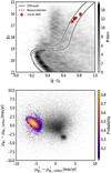 |
Fig. 1. Top panel: Hess diagram of stars selected in reflex corrected PM space following Bonaca et al. (2019b), and with |ϕ2|< 2 deg and RUWE < 1.4. The diagram has been smoothed using a 0.4 mag Gaussian kernel. The dashed line shows the selection from the same authors, while the solid line shows that adopted in this work. Our selection is based on a 12 Gyr, [Fe/H] = −1.7 PARSEC isochrone at a distance of 13 kpc. The red circles show confirmed stream members from Ji et al. (2020). Bottom panel: reflex corrected PM for stars selected according to the CMD mask shown above. Jhelum candidates are coloured coded by their membership probability. |
Using this CMD selection, we modelled the distribution in the reflex motion corrected PM space as a 6 component Gaussian mixture model2 (Bovy et al. 2011), using the full co-variance matrix (and again imposing that |ϕ2|< 2 deg, and RUWE < 1.4). After this step, we evaluated the Jhelum membership probability for all stars in our initial sample while relaxing the |ϕ2| selection criterion. In the bottom panel of Fig. 1, we show the PM distribution of all stars in our sample, where Jhelum candidate stars are colour coded according to their membership probability (provided this is larger than 10%).
2.1. Narrow component member selection
In Fig. 2, we show stars with a membership probability higher than 50% and with a parallax < 0.8 mas. Especially the smoothed density map plotted in the lower panel of this figure clearly shows that Jhelum consists of a narrow component centred around ϕ1 ≈ 0.5 deg and an extended broader component beneath it. Moreover, we find a third, yet unreported component above the narrow one around ϕ1 ≈ 0 – 5 degrees. The main narrow component has a clumpy morphology with several tentative gapsand some overdensities, most notably at ϕ1 = −1 and 16 deg. Finally, we note that there seems to be a discontinuity in the narrow component at ϕ1 ≈ 14 deg. We conclude that Jhelum has a very complex morphology, with many of the features seen in Gaia DR2 (Bonaca et al. 2019b) now more clearly apparent thanks to the better astrometric quality of Gaia EDR3.
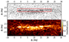 |
Fig. 2. Positions in (ϕ1, ϕ2) of stars with a membership probability larger than 50% and parallax < 0.8 mas displayed as a scatter plot (top) and a smoothed density map (bottom). Jhelum clearly stands out as an overdensity and has a clumpy morphology with multiple gaps. Possible narrow-component members are contained within the red region in the top panel. Below this region, the extended broad component stands out, while above it, between ϕ1 ≈ 0–5 degrees, a thus far unreported third component can be seen. |
Bonaca et al. (2019b) fitted the median location of the narrow component as a function of ϕ1 as
 (1)
(1)
where ϕ1 and ϕ2 are in degrees. Therefore, we select as tentative narrow-component members those stars with membership probability higher than 50% and parallax < 0.8 mas that lie within  degrees of the median within the range −2.5 ≤ ϕ1 ≤ 22.5 deg.
Of the nine confirmed Jhelum stream members with radial velocity measurements from Ji et al. (2020), Sheffield et al. (2021), we spatially selected the four stars with ϕ2 > 0.2 deg as possible narrow component (NC) members. These are the stars Jhelum2_2, Jhelum1_5, Jhelum2_11 and Jhelum2_14 from Ji et al. (2020). Throughout this work, we refer to these stars as RV-NC-stars. The other five stars, Jhelum_0, Jhelum1_8, Jhelum2_10 and Jhelum2_15 from Ji et al. (2020) and the APOGEE Jhelum giant from Sheffield et al. (2021), are assumed to belong to the broad component (BC) and are referred to as RV-BC-stars. The RV-NC-stars and RV-BC-stars are shown in Fig. 3 in blue and orange respectively.
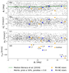 |
Fig. 3. Stars with a membership probability larger than 50%, parallax < 0.8 mas and 5 ≤ ϕ1/deg ≤ 25, −3 ≤ ϕ2/deg ≤ 3 are shown as black dots in (panel a) on the sky (ϕ1, ϕ2), in (b) in (ϕ1, |

2.2. Characterization of the Jhelum stream track
To characterize the Jhelum stream and its track in PM, the positions and PM of the possible narrow-component members (i.e. inside the box shown in Fig. 2) were binned in ϕ1 with a binsize of 5 deg and a stepsize of 2.5 deg. In each ϕ1-bin we fitted a Gaussian distribution with a constant background B, given by
 (2)
(2)
for each observable x, that is to say ϕ2,  , or μϕ2, and where A is the relative normalization of the Gaussian component, μx is the mean and σx is the dispersion. We used the minimization implementation from scipy.optimize.minimize to determine the various parameters in Eq. (2), all of which are allowed to vary from bin to bin.
To avoid that particularly high density regions end up with unrealistically low uncertainties, after fitting we checked that in each ϕ1-bin, σϕ2 is greater than the average ⟨σϕ2⟩ determined using all ϕ1-bins. If this is not the case, we assigned it this average. This floor in σϕ2 can be seen as a way to reduce the impact of the clumpiness in Jhelum’s narrow component when characterizing the stream track.
The resulting stream track is shown in Fig. 4, where the shaded region denotes the extent defined by 1σ around the mean estimated as just described. We note that in the top panel there is a jump in the stream track on the sky around ϕ1 ≈ 14 deg (see also Fig. 2), i.e. for ϕ1 < 14 degrees, the track is approximately constant at ϕ2 ≈ 0.5 deg, while for ϕ1 > 14 deg, it is approximately constant but now at ϕ2 ≈ 0.9 deg.
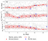 |
Fig. 4. Distribution of high probability narrow component members (> 50%) in (a), (ϕ1, ϕ2), (b), (ϕ1, |

3. Orbit fitting
We now aim to determine if there are orbits which, when integrated in a MW potential, approximately follow the track defined by the Jhelum stream. Although we do not expect a stream to exactly follow a single orbit (see Sanders & Binney 2013, for a detailed discussion), it turns out that for Jhelum, this is not a bad approximation (see Appendix A).
To establish the characteristics of such an orbit, we defined a log-likelihood which yields the probability that the single orbit fits each datapoint i, given the uncertainties in the data and the internal dispersion of the stream, namely
![Mathematical equation: $$ \begin{aligned} \ln (L)&= \frac{1}{N} \sum _{i}^N \ln (L_i) \nonumber \\&= \frac{1}{N} \sum _{i}^N \left[- \ln \left(\prod _{j=1}^{4} (2 \pi )^{1/2} \sigma _{i,j} \right) - \frac{1}{2} \sum _{j=1}^{4} \left( \frac{x_{i,j}^d - x_{i,j}^m}{\sigma _{i,j}} \right)^2 \right] \end{aligned} $$](/articles/aa/full_html/2023/01/aa43266-22/aa43266-22-eq9.gif) (3)
(3)
where j represents the subspace δ,  , μδ or vrad. The superscripts d and m denote the data and model respectively. The datapoints consist of the means and dispersions obtained using the fitting procedure described in the previous section, as well as the measurements for the individual RV-NC stars. For the RV-NC stars’ astrometry, we added in quadrature to their measurement uncertainties the average values of ⟨σ⟩ for ϕ2,
  , and μϕ2 as derived in the previous section. This is done to account for the observed dispersion in the stream, which is not reflected in the measurement uncertainties of the individual stars.
To estimate the uncertainties in the RV-NC stars’ radial velocities we proceed as follows. We not only considered the measurement error, but also that the stream might have an internal velocity dispersion, so  . The nuisance parameter, σnuis, has two components: a random σrand, and a systematic σsyst, which are added in quadrature. The systematic component was determined by taking the average of the difference in radial velocity measurements by AAT and MIKE of the 8 Ji et al. (2020) stars (see Table 1 in Ji et al. 2020), while leaving out Jhelum2_2 because it is probably a binary star. This gives σsyst = 1 km s−1, which is consistent with the median velocity offset found by Ji et al. (2020). The random component was determined by considering three pairs of stars that lie close together on the sky, Jhelum_0 and Jhelum2_2 around ϕ1 ≈ 6 deg, Jhelum1_8 and Jhelum2_10 around ϕ1 ≈ 11 deg, and Jhelum2_14 and Jhelum2_15 around ϕ1 ≈ 22 deg, and by measuring their radial velocity difference. We then set the random velocity to be the mean of these differences which gives σrand = 6.6 km s−1. Finally, σnuis = 6.7 km s−1.
We note that this value of σnuis is likely an upper limit to the internal dispersion of the stream. In practise, a large value allows a more generous range of the free parameters that are fitted, as can be seen from Eq. (3). This is why we also considered a more realistic 2 km s−1 for σnuis in what follows (Kuzma et al. 2015; Malhan & Ibata 2019; Gialluca et al. 2021).
To start the orbit integrations, we assumed a fixed right ascension of α = 330 deg, which corresponds to (ϕ1, ϕ2) ≈ (18.7, 0.8) deg in the stream-aligned coordinate system. For the other coordinates, we set a flat prior given by
 (4)
(4)
As we have no reliable information on the distances to the stars, we left this as a free parameter within the range of the prior. For the potential, we first assumed a standard MW mass model (see Sect. 3.1), and we then explored what happens when its characteristic parameters are allowed to change (see Sect. 3.2) using the package AGAMA (Vasiliev 2019).
3.1. Best-fit orbit in a standard Milky Way potential
We modelled the MW gravitational potential as a three-component system consisting of a bulge, disk, and dark halo, following Price-Whelan et al. (2020). The bulge was modelled as a Hernquist sphere (Hernquist 1990) with a mass of 4 × 10⁹ M⊙ and scale length cb = 1 kpc. The disk was modelled as a Miyamoto-Nagai potential (Miyamoto & Nagai 1975) with Mdisk = 5.5 × 10¹⁰ M⊙, scale length ad = 3 kpc, and scale height bd = 280 pc (Bovy 2015). The dark halo follows a generalized Navarro-Frenk-White (NFW) potential (Navarro et al. 1996), which can be made spherical, flattened or triaxial by changing the values of the axis ratios. We set the scale radius rs = 15.62 kpc, Mhalo = 0.7 × 10¹² M⊙, and the halo potential to be flattened with a minor-to-major axis ratio qz = 0.95.
Using this potential, we performed a Markov Chain Monte Carlo (MCMC) with the package emcee (Foreman-Mackey et al. 2013) to find the orbit (model) parameters that fit the data best, where we use 80 walkers and 1000 steps. As α is fixed, there are thus five free parameters to be explored by the MCMC algorithm, (δ, d,  , μδ, vrad). An initial guess that was used in the MCMC was found using scipy.optimize.
The MCMC chains converged regardless of the choice of σnuis. The resulting posterior parameter distribution obtained for σnuis = 6.7 km s−1 is shown in Fig. 5. The posterior parameter distribution for σnuis = 2 km s−1 is similar but tighter, especially in radial velocity. Figure 5 reveals that there is a strong degeneracy between the distance and μδ, and weaker degeneracies between the distance and vrad and between μδ and  . The best-fit orbit for σnuis = 6.7 km s−1 has an apocenter of 23.6 kpc and pericenter of 8.1 kpc (similar values are found for σnuis = 2 km s−1), where the apo- and pericenter are calculated by averaging them over an integration time of 10 Gyr. Interestingly, although Bonaca et al. (2019b) did not take radial velocity information into account, they obtain a similar best-fit orbit, with an apocenter of 24 kpc and a pericenter of 8 kpc.
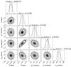 |
Fig. 5. Posterior parameter distribution of the initial conditions of the best-fit orbit of Jhelum for σnuis = 6.7 km s−1 in the default MW potential. We note the (expected) strong degeneracy between the distance and μδ. |
The best-fit orbits follow well the positions and PMs of the stream, see panel (a)–(c) of Fig. 6, though Jhelum2_14 deviates by about 2σ in μϕ2 from the best-fit orbit. In fact, Jhelum2_14 was already seen to deviate from the stream track in Fig. 4.
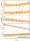 |
Fig. 6. Best-fit single orbit of Jhelum in the default MW potential for σnuis = 6.7 km s−1 (dark blue line) and σnuis = 2 km s−1 (dashed light orange line). 100 orbits were sampled randomly from the MCMC chains for the higher and lower values of σnuis, and are shown in light indigo and in orange respectively. The binned estimates and their 1σ uncertainties are plotted in red, while the individual RV-NC-stars (along with their names) are plotted in blue for σnuis = 6.7 km s−1 (and light-blue for its smaller value). Though the orbits follow the binned track and RV-NC-stars well within the error bars in position and PM, in radial velocity no orbits go through all of the four RV-NC stars: Jhelum2_14 and especially Jhelum1_5 lie far outside the sampled range in radial velocity. The distance to the stream is somewhat low in comparison to the estimate by Shipp et al. (2018), but consistent with the estimate by Li et al. (2022). |
The distance distribution is consistent with the recent estimate by Li et al. (2022), but slightly below the estimate by Shipp et al. (2018), see panel (d). Figure 6 also shows a sample of 100 orbits, randomly selected from the posterior distribution of initial conditions. No single orbit is capable of going through all the radial velocity measurements of the RV-NC stars, with Jhelum2_14 and Jhelum1_5 being the most deviant ones. This is the case regardless of the σnuis adopted.
3.2. Varying gravitational potential parameters
We explored if by varying parameters of the Galactic gravitational potential we are able to fit the data on the Jhelum stream better. We kept the bulge and disk the same as in the default MW potential, and let the halo be triaxial, where the axis ratios denoted as qx = a/b, qz = c/b, the scale radius rs and its mass Mhalo are all allowed to vary. We restricted ourselves to potentials that give rise to a correct velocity at the position of the Sun within 5% assuming Vcirc(R⊙) = 233 km s−1 (Reid et al. 2014; McMillan 2017; Hayes et al. 2018; Eilers et al. 2019; Mróz et al. 2019)3. We also required that the density of the NFW halo component is positive over the extent of the MW (−300 < x, y, z < 300 kpc). These two constraints limit the extent of the parameter space that the MCMC is allowed to explore. As the parameters qx and qz but also rs and Mhalo are correlated in non-trivial ways, we chose somewhat generous flat priors as a starting point, namely 0.7 < qx < 1.4, 0.7 < qz < 1.4, 3 × 10¹¹ < Mhalo < 3 × 10¹²M⊙ and 10 < rs < 25 kpc. We then checked that both constraints were satisfied by the MCMC chains.
Together with the parameters associated to the orbital initial conditions (δ, d,  , μδ, vrad), we thus have a total of 9 free parameters to be determined by the MCMC. As the parameter space to be explored by the MCMC has increased, we used 80 walkers and 2000 steps. We only considered the σnuis = 6.7 km s−1 case as this serves effectively an upper limit on the allowed range of the free parameters. The resulting posterior parameter distribution is shown in Fig. 7, where that of the orbital initial conditions resembles that obtained for the default MW potential fit and shown in Fig. 5. Figure 7 shows that there is a strong degeneracy between Mhalo and the scale radius rs, which is partly induced by the circular velocity constraint. qx and qz are also correlated in a non-trivial manner, which is largely determined by the positive density constraint. In comparison to the default halo potential model, a larger scale radius, rs = 19 kpc, in combination with a larger halo mass, Mh = 1.0 × 10¹² M⊙, seem to be preferred, as well as an almost spherical halo, with qx = 1.04 and qz = 1.024.
 |
Fig. 7. Posterior parameter distribution of the initial conditions of Jhelum’s best-fit orbit and of the parameters of the Galactic halo potential, for σnuis = 6.7 km s−1. We note that here, the bulge and disk were kept fixed and set to be those of the default MW potential. The posterior parameter distribution of the initial conditions resembles the one of the default MW potential shown in Fig. 5. There is a strong degeneracy between Mh and rs, as expected, and is a result of the circular velocity constraint. The correlation between qx and qz is set by the requirement that the halo density be positive. |
The best-fit single orbit, as well as 100 orbits sampled randomly from the MCMC chains are shown in Fig. 8. For comparison, the best-fit orbit in the default MW potential is shown as well. From Fig. 8 it is clear that allowing the parameters of the potential to vary does not result in a significantly different best-fit orbit (although the data is generally fitted better as with the additional degrees of freedom there are more high-likelihood values). In fact, the two best-fit orbits closely resemble each other in all subspaces. We find again that the best-fit orbits follow the positions and PMs well (with Jhelum2_14 still deviating by more than 2σ from the best-fit orbit in μϕ2). On the other hand, in radial velocity Jhelum2_14 and Jhelum2_2 lie consistently 10 − 20 km s−1 below the best-fit orbits and on the edge of the sampled range, while Jhelum1_5 lies far above it, ∼50 km s−1. In conclusion, there is no potential that fits the data perfectly, and in particular the radial velocities cannot be matched, independently of the values of the characteristic parameters or shape of the Galactic potential used.
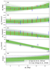 |
Fig. 8. Best-fit single orbit of Jhelum for the default MW potential (dark blue line) and the MW potential with triaxial halo (dashed light green line) for σnuis = 6.7 km s−1. 100 orbits sampled randomly from the MCMC chains are shown using the same colour as the corresponding best-fit orbits. We note that allowing parameters of the Galactic potential to vary given the constraints does not yield significantly different orbits. |
3.3. The effect of perturbers: an encounter with Sagittarius
Jhelum is a peculiar stream with multiple components showing over- and underdensities (see Fig. 2). It is perhaps in hindsight not so surprising that no single orbit in a realistic Galactic gravitational potential can be found that matches the track of the narrow component of the stream well.
In search for an explanation, we considered the possibility that Jhelum has been perturbed while orbiting the MW. We focused in particular on the influence of the two heaviest dwarf satellites galaxies of the MW, namely the LMC and Sgr.
To check whether these objects might have come close enough to Jhelum to perturb it, we integrated, using the default MW potential, the orbit of the LMC including dynamical friction, that of Sgr and Jhelum’s best-fit single orbits (for both values of σnuis) separately 6 Gyr back in time. The initial conditions for the orbit integrations of Sgr and the LMC are listed in Table 1. We then calculated the distance at the closest passage between the centre of mass of Jhelum (which we considered to be located on the best-fit orbit) and these objects. In the case of the LMC, and being on its first infall, the closest passage with Jhelum is at the present time at a relative distance of 44 kpc, and although this might have an effect on its dynamics (see e.g. Shipp et al. 2021), such an interaction would not explain its disturbed morphology as substructure would need more time to form. To further assess the effects of the LMC in conjunction with Sgr, we investigated their combined influence in Appendix B. We find again that the LMC’s influence only becomes significant recently, which is in line with the findings of Shipp et al. (2021).
Orbital properties of the LMC and M54 (which is used to trace Sgr’s orbit).
On the other hand, Jhelum and Sgr passed each other closely multiple times over the past 6 Gyr, with distances at closest passage ranging from 3 − 6 kpc. Figure 9 shows the orbit of Jhelum and Sgr both integrated for 6 Gyr back in time and reveals that these objects seem to share a similar orbital plane, which explains why they have repeated close encounters. This is also the case for the MW potential fitted in Sect. 3.2. The periodic character of these interactions suggests that Sgr might have had a considerable influence on Jhelum, and that this could perhaps explain its orbit and the observed peculiar stream morphology.
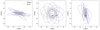 |
Fig. 9. Best-fit orbit of Jhelum in the default MW potential (for σnuis = 6.7 km s−1) plotted together with the orbit of Sgr (using the coordinates of M 54, see Table 1), both integrated backwards in time for 6 Gyr. The arrows indicate the direction in which Jhelum and Sgr are currently moving. It is clear that Jhelum and Sgr share approximately the same orbital plane, which results in repeated close encounters between the two. We note that Jhelum is currently passing through pericenter, which is the reason for the high observed velocity gradient seen in Fig. 8. |
In the case of the LMC, and being on its first infall, the closest passage with Jhelum is at the present time at a relative distance of 44 kpc and although it might have an effect on its dynamics, such an interaction would not explain its disturbed morphology.
4. Study of the Sgr-Jhelum interaction
In this section, we further investigate the possibility that Jhelum was perturbed by Sgr. To this end, we performed N-body simulations of the interaction between the progenitor of Jhelum and Sgr while they orbit the Galaxy.
4.1. Choice of initial conditions
To explore a set of reasonable orbital initial conditions for the progenitor of Jhelum we created a bundle of possible orbits around one Jhelum member, Jhelum2_2, which we set to represent the present-day position of the progenitor. We used α and δ from Jhelum2_2 and sampled  and μδ from a Gaussian distribution with σ given by the error estimated in Sect. 2.2. For the distance we sampled from a uniform distribution between 10.6 kpc and 14.6 kpc, corresponding to the value reported for the Jhelum member in Sheffield et al. (2021) and compatible with photometric distance estimates to the stream. We sampled the initial radial velocity from a Gaussian distribution with mean and variance from the observed RV-NC stars, excluding Jhelum2_14 and Jhelum2_15 which deviate from the seemingly linear velocity trend (see Fig. 3). The sampling intervals for our bundle of orbits are collected in Table 2.
Sampling parameters for the initial conditions of the orbit integrations of Jhelum and the parameters of the four selected orbits used for the N-body experiments integrated with GADGET-4. For these integrations, α and δ were kept at a fixed value.
We then integrated the orbits generated this way backwards in time, in the same Galactic potential as described in Sect. 3.1. We now also included the potential associated to Sgr. For Sgr, we used the orbital initial conditions listed in Table 1. As a starting point, we fixed the mass of Sgr initially to 3 × 10⁹ M⊙ and assumed that it follows a Plummer profile with a scale radius of ∼1 kpc, based on a rescaling of the model in Laporte et al. (2018) after converting to a Plummer sphere with a similar concentration parameter (as in Appendix B of Koppelman & Helmi 2021).
Before deciding which of the generated initial conditions for Jhelum may be most interesting for the N-body simulations, we explored the orbits further. Firstly we considered only those orbits that reasonably reproduce the track of Jhelum on the sky. The interpolated orbit (for each initial condition generated as described above) was compared to the observed stream track using the quantity D2, defined as
 (5)
(5)
where ϕ2, pol is the polynomial from Eq. (1) and N = 40 is the number of points where the polynomial is compared to the orbit.
We consider orbits with D2 < 0.2 to follow the stream track well (top 1.73% of the 50 000 generated initial conditions). We note that since D2 is calculated using on-sky angular distances, there is a bias towards preferring orbits with a larger distance, as we see below. During our orbit integrations we kept track of the minimal relative distance and relative velocity to Sgr. We focus on interactions with Sgr that occurred more than 2 Gyr ago, as more recent ones would likely not produce easily visible perturbations in the stream as the timespan is too short, and also because Sgr would likely be lighter and hence have a smaller impact (e.g. Vasiliev & Belokurov 2020). From this sample, we selected four orbits that come closer than 6 kpc to Sgr and which, as we show below, produce interesting features in the Jhelum stream. The resulting initial conditions for Jhelum are collected in Table 2.
4.2. Simulation setup
While previous works conclude that Jhelum most likely had a DG progenitor (e.g. Li et al. 2022; Shipp et al. 2019; Bonaca et al. 2019b; Ji et al. 2020), we choose to take a (loose) GC progenitor. We do this because the narrow component of Jhelum has a width comparable to that of other cold streams (e.g. Shipp et al. 2018) and our goal is to fit the narrow component while perturbing the stream to produce the observed features. The progenitor follows a Plummer sphere of scale radius 9 pc with a mass of 5 × 10³ M⊙, and consists of 5 × 10³ particles, and was generated self-consistently using AGAMA (Vasiliev 2019). The chosen scale radius is typical for observed GCs (de Boer et al. 2019), while the mass is somewhat lower (Baumgardt & Hilker 2018), to allow for a cold enough stream with a fully dissolved progenitor after 6 Gyr of evolution.
To model the interaction between Jhelum and Sagittarius, one would perhaps like to resort to full N-body simulations representing Jhelum and its stream, Sgr, and the underlying Galactic potential. This is however prohibitive, as this would require these systems to be represented by particles with comparable masses to prevent artificial heating in the (newly formed) stream (see Banik & Bovy 2021). Given the mass of Jhelum and the desired resolution in its stream, this implies mp ∼ M⊙. This would require 1012 particles for the MW halo (and ∼109 particles for Sgr). Since the use of currently computationally feasible simulations (with mp ∼ 103 − 105 M⊙) would incorrectly model the gravitational potential of the MW, we prefer to use the analytic description presented in Sect. 3.1.
A full N-body realization of Sgr would have the advantage of accounting for mass loss, which may have an effect on the strength of the interactions with Jhelum. Therefore, to still model the mass loss of Sgr, we first ran an N-body simulation of Sgr evolving on its own in the background MW potential. We then used this simulation to calibrate a time-dependent analytic Plummer potential of Sgr as this evolves. This was subsequently employed in a forwards N-body simulation of Jhelum to model Sgr as one particle with a softening scale and mass determined by the Plummer parameters at each point in time.
For the N-body simulations of Sgr, we used AGAMA to generate 105 particles according to a self-consistent distribution function belonging to the Plummer sphere from Sect. 4.1, and let it dynamically relax for ∼6 Gyr. We then carried out the N-body simulation of Sgr in the MW potential integrating forwards in time for ∼6 Gyr. We used GADGET-4 (Springel et al. 2021) with SELFGRAVITY enabled, and included the background MW potential using the EXTERNALGRAVITY flag. At each snapshot, we fitted an analytic Plummer potential given by
 (6)
(6)
to the distribution of particles still bound to the progenitor. This results in a tabulated mass and scale radius for Sgr through time. We fit this evolution in time with smooth polynomials. This then allowed us to represent closely the behaviour of a live Sgr evolving in a Galactic potential. We show the evolution of the parameters of our Sgr model through time in Appendix C.
We performed our N-body simulations of the Jhelum stream with the same configuration for GADGET-4 (Springel et al. 2021) as before. We considered two particle types: one for Jhelum stars and one for the single particle representing Sgr. For the Sgr particle, we adopted a softening parameter equal to its fitted scale radius, which in practise corresponds to the Plummer sphere representing Sgr. The softening length for the Jhelum particles was set to 2 pc (determined using the methodology of Athanassoula et al. 2000; Villalobos & Helmi 2008). We proceeded in two steps. We first integrated Jhelum starting from the initial conditions selected in Sect. 4.1 backwards with the mass varying Sgr particle. Then we replaced the Jhelum particle with a relaxed progenitor and integrated forwards again. In all our simulations we allow a maximum timestep of 0.49 Myr, with a default ErrTolIntAccuracy of 0.012.
To study the specifics about the stream-formation process, we monitored the history of mass loss. We defined the centre of mass of the progenitor by taking the mean position of the 200 particles with the highest binding energy (identified initially, i.e. in the relaxed progenitor), and keeping track of those that remain within the tidal radius rt at all times. The tidal radius was calculated by using the constraint that the equipotential surface between the background potential (ρbg) and the progenitor (ρprog) occurs at the tidal radius, that is to say ρprog(rt)=3ρbg(rperi), where rperi is the pericentric distance of the progenitor. In our case, this results in rt = 18 pc. Whenever a particle crosses the tidal radius for the last time in the simulation, we say it has become unbound. We record the following pericenter passage of the progenitor as the release time of the particle.
4.3. Tracking and characterization of the interactions
Close interactions between Sgr and Jhelum may result in velocity kicks to the stream members. Such kicks can generally be described using the impulse approximation. If the impact parameter is b (i.e. the distance between the perturber and the point of closest impact on the stream) and the stream is aligned with the y-direction, the maximal total velocity kick Δv imparted at a given point is
 (7)
(7)
where M is the mass, and rs the scale radius of the perturber. Here  , with w∥ the relative y-velocity of the perturber along the stream and
  , with wx, z the respective components of the velocity of the perturber. We refer the reader to Carlberg (2013) and Erkal & Belokurov (2015) for general expressions for the velocity impulse experienced by stream particles due to the passage of a perturber.
To monitor the amplitude of the velocity kicks and the location of the closest encounters, we first identified the snapshots where the distance between Sgr and the Jhelum progenitor is smallest. Then we searched in the neighbouring (five preceding and following) snapshots and identified the snapshot where the largest number of particles are close to Sgr. The point at which this occurs is used to label the time of the interaction and to compute the velocity kick experienced by those particles.
4.4. Results
Figures 10–13 show the present-day properties of the simulated streams using the 4 orbits described in Sect. 4.1. These figures show that interactions with Sgr could certainly explain the observed multiple components structure of the Jhelum stream reported in Bonaca et al. (2019b) and also seen in Fig. 2. The simulated streams have narrow components with widths comparable to the observations. Furthermore, although the stream generally extends beyond ϕ1 = [ − 10, 30] deg in our simulations, such portions of the stream are more diffuse, more sparsely populated or even completely ‘folded’ over, explaining why they may have not yet been detected. This may also apply to some of the subcomponents seen in these figures, which would perhaps not be apparent with current datasets, as their density may be too low.
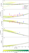 |
Fig. 10. Simulation 1 of the Jhelum stream after interacting with the Sgr dwarf spheroidal. The individual star particles from Jhelum are colour-coded according to the lookback time at which they became unbound. Panel a: shows the stream in ϕ1-ϕ2 frame, while (panels b) and (c) show the (non-reflex corrected) PM in the ϕ1 and ϕ2 directions respectively. Panel d: radial velocity, and Panel (e) the distance. The red datapoints correspond to the binned Jhelum data from Sect. 2.2, and the blue datapoints correspond to stars from Ji et al. (2020) that are likely members of the narrow component of Jhelum. The magenta triangle corresponds to Jhelum2_2, the datapoint which in our simulations marks the present-day location of the progenitor. The magenta dotted line shows the trajectory of the centre of mass of the Jhelum progenitor, and the grey dashed line shows the result from the MCMC best-fit with σnuis = 6.7 km s−1 from Sect. 3.1. Panel a: clear secondary and tertiary components, which are also apparent in the other panels. These additional components are made up of particles that were released early on in the formation of the stream. |
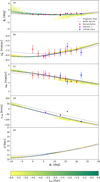 |
Fig. 11. As Fig. 10, but now for Simulation 2. The bottom component is short, dense and close to the narrow component. To the left, the leading tail shows signs of a diffuse tertiary component that is the result of a ‘folding’. |
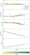 |
Fig. 12. As Fig. 10, but now for initial conditions 3. The trailing tail has completely folded over and shows up as the component on top of the narrow component, and the leading tail shows up as a tertiary component to the bottom of the narrow component on the left of the figure. The two additional components are clearly visible in μϕ2. |
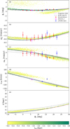 |
Fig. 13. As Fig. 10, but now for initial conditions 4. Here in Panel (a) we see a more diffuse secondary component in the bottom, and a tertiary component in the top, see for comparison to Figs. 10–12. This stream also has a very clear separation of the components in vrad, even fitting Jhelum1_5. |
A remarkable feature of all additional components is that they seem to be formed by particles that were released from the progenitor quite early during the formation of the stream (i.e. the yellow particles in Figs. 10–13). This means that the interaction(s) with Sgr cause the tail(s) of the stream to end up closer to the progenitor (located at ϕ1 = 5.8 deg) than they would if the stream had evolved in a smooth potential.
The diversity of the streams revealed in Figs. 10–13, particularly in terms of the morphology and number of subcomponents, shows that the specifics of the encounters leave different kinds of imprints on the stream. To shed light on this, we studied the history of the stream and characterized the interactions as described in Sect. 4.3. To establish exactly which encounter is responsible for a specific morphological feature we ran additional simulations where we removed Sgr after each interaction, so that we could isolate the effect of a single encounter (in practise we removed Sgr when it is maximally distant from Jhelum after the interaction) and evolved Jhelum in isolation for the remainder of the time. We can thus record the impact of each interaction before adding the next interaction to finally study the combined effect.
The first close interactions in our simulations occur typically before tlookback = −5.1 Gyr. Regardless of the velocity kick imparted, these interactions do not correspond with any visible substructure in the resulting stream. This is because the stream barely started forming at this point in time in our simulations.
Interestingly, the most impactful interactions (whose properties are listed in Table 3) correspond to close passages of Sgr to the stream that have a differential effect. They impart the highest Δv locally, and simultaneously impart velocity kicks of different amplitude to different portions of the stream. This gradient in Δv causes the two tails to get a different velocity kick compared to each other, and to the progenitor. After the interaction the progenitor continues disrupting, forming new tails. This is why we often observe three components in the case of an impactful interaction. One component corresponds to the portion of the stream formed after the interaction, while the other two components are the tails of the stream already present at the time of the interaction.
Parameters of the most impactful interactions between Jhelum and Sgr.
After one impactful interaction has perturbed the original tidal tails, causing them to start precessing around the orbit of the progenitor, further close interactions with Sgr can still occur. Because the stream is now a more extended object, it is easier to create a difference in Δv between the new stream and the two perturbed original tails. The perturbed tails are subject to a higher or lower Δv than the particles in the newly formed tidal tails from the progenitor, which generally do not experience a gradient in Δv in these interactions. Therefore, while these interactions will have an effect on the morphology of the stream at present time, they will generally not create additional substructure.
The orbital phase of each interaction also has an impact on its outcome, in the sense that interactions closer to pericentre are more likely to produce a larger gradient in Δv due to the contraction of the stream in this orbital phase. Furthermore, the geometry of the interaction itself is also important for the present-day on-sky visibility of the resulting substructure. We now proceed to describe in detail the characteristics of each one of the simulations shown in Figs. 10–13.
4.4.1. Simulation 1
This stream, shown in Fig. 10, is particularly interesting because it shows three clear components in the ϕ1 − ϕ2 plane, that is to say on the sky. One corresponds to the expected narrow component, which we also call the main component. There are additional components above and below the main one, that could correspond to the components seen in the data and shown in Fig. 2. These additional components also show up in the ϕ1 − μϕ1 and the ϕ1 − μϕ2 plane, separated from the main component by up to Δμϕ2 ∼ 0.2 mas yr−1. They are also visible in the ϕ1 − vrad plane, but then separated by up to Δvrad ∼ 30 km s−1.
In this simulation, four close interactions with Sgr happen, only one of which, the one at −3.1 Gyr, is the main cause of the observed substructure. This interaction imparts a kick of ∼14 km s−1 to the bottom component, ∼8 km s−1 to the main component and ∼4 km s−1 to the top one, due to passing closer to the trailing tail. The narrow component is approximately 9× as dense as the top component, and 12× denser than the bottom component at the present time.
4.4.2. Simulation 2
This stream, plotted in Fig. 11, is specifically interesting because it shows only one clear secondary component, which is 2.5× more diffuse than the main component, although the leading tail shows up as a diffuse folded over component at ϕ1 ∼ −10. The length of the bottom component does not exactly match that reported in Bonaca et al. (2019b), which can be explained by the unknown position of the progenitor, which in our simulation is located far to the left in ϕ1. The second component is also visible in the  , μϕ2 and vrad panels of Fig. 11 as a broader part of the stream. The diffuse leading arm has a similar in origin to the observed tertiary component, which is approximately in the same location.
The morphology found in this simulation is mainly due to one interaction (see Table 3). The secondary component is made up from the trailing tail of the stream, where the leftmost part consists of particles that were released in the first pericentric passage. This encounter at ∼ − 4.3 Gyr imparted a velocity kick of ∼2 km s−1 to the particles in the leading tail, which should be compared to the kick of ∼6 km s−1 to the particles in the main component and ∼9 km s−1 to the particles in the second component. The other reported passage in Table 3 enacts a velocity kick of ∼7.5 km s−1 to the particles in the trailing tail and the already folded over second component, ∼6 km s−1 to the progenitor and ∼4 km s−1 to the leading tail, which was already slightly folded over and more diffuse at this time. This reinforces the fact that not all close interactions necessarily cause substructure. Especially later interactions only enact a differential Δv among the three components of the stream because of the already existing substructure.
4.4.3. Simulation 3
This stream, shown in Fig. 12, again shows three components, one below and one above the narrow component. It is interesting because it matches the observed substructure quite closely when mirrored around ϕ2 = 0, and because the trailing tail is fully truncated and folded over and shows up above the narrow component. The bottom component is also visible in μϕ2 as a broader part of the stream, while the top component is only clearly separated from the narrow component in μϕ2, by Δ μϕ2 ∼ 0.1 mas yr−1. The bottom component is made up of particles from the leading tail while the top one by particles from the trailing tail. These subcomponents formed after one interaction at −2.5 Gyr, where Sgr passes closest to the middle of the leading tail and imparts a velocity kick of Δv ∼ 15 km s−1 to the leading tail, ∼10 km s−1 to the progenitor and ∼5 km s−1 to the trailing tail. The narrow component is equally dense as the top component, and 8× more dense than the bottom one.
4.4.4. Simulation 4
The stream plotted in Fig. 13 has a narrow component that is ∼10× denser than the top component, and 2× than the bottom one. This latter component is visible in μϕ2 and vrad, separated by up to Δμϕ2 ∼ 0.2 mas yr−1 and Δvrad ∼ 25 km s−1 from the narrow component, while the top component is separated in  , μϕ2, vrad and distance by up to Δ
  ∼ 0.1 mas yr−1, Δ μϕ2 ∼ 0.4 mas yr−1, Δ vrad ∼ 50 km s−1 and Δ d ∼ 0.2 kpc.
The bottom component is made up of particles from the trailing tail, while that in the top consists of those from the leading tail. These components formed through two interactions, whose specifics are collected in Table 3. The first interaction causes the existing tails to start precessing around the orbit, but this does not show up in the ϕ1 − ϕ2-coordinates because the velocity kick was mainly imparted in the radial direction. The second interaction then imparts a kick that separates the tails visibly in ϕ1 − ϕ2. In this case the closest passage of Sgr is with the middle of the leading tail, imparting a kick of up to ∼14 km s−1, while the progenitor and the trailing tail receive kicks of ∼7 km s−1 and ∼3 km s−1 respectively.
5. Discussion and conclusions
With the new Gaia EDR3 data, we unveil new structures in the Jhelum stellar stream. This has been possible thanks to the smaller PM uncertainties in EDR3 as well as to a more sophisticated selection technique. Besides the clumpy nature of the stream and its narrow and broad components (first reported in Bonaca et al. 2019b), we find evidence for a third, also broad component above the stream main track. Additionally, we find a kink-like feature (at ϕ1 ≈ 14 deg) in the narrow component of the stream. After submission of this manuscript, these findings were confirmed by Viswanathan et al. (in prep.) using a reduced PM halo catalogue.
Such kinks are generally expected around the location of the progenitor, marking the transition from the leading to the trailing arm. However, in the case of Jhelum, the leading arm (extending towards ϕ1 < 0) would be expected to be above the average stream track, while the trailing (extending towards ϕ1 > 0) would be expected to be below it, which is the opposite of what we observe. The kink is thus more likely due to a perturbation by a substructure. In fact, this has been proposed to explain the wiggle seen in the GD-1 stream (de Boer et al. 2020), and the kink feature observed in the ATLAS-Aliqua Uma stream (Li et al. 2021), which although of larger amplitude than observed in Jhelum, has also been attributed to a close interaction with Sgr.
When characterizing Jhelum’s narrow component, we find the stream track to be best described by the polynomial
 (8)
(8)
which differs slightly from that reported by Bonaca et al. (2019b). For comparison, both tracks are plotted in Fig. 14, which shows that the Bonaca et al. (2019b) polynomial is not curved strongly enough to follow the binned track of the stream. To supplement the stream track data, we used the publicly available S5 (Ji et al. 2020) and APOGEE (Sheffield et al. 2021) data, which provide radial velocity data for 9 confirmed Jhelum members. Out of these, 4 stars can be associated to Jhelum’s narrow component.
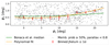 |
Fig. 14. Possible narrow component members in (ϕ1, ϕ2). The binned track with 1σ uncertainty range are indicated in red. The polynomial fitted to this track, Eq. (8), is shown in orange. For comparison, the Bonaca et al. (2019b) median is overplotted in green. The updated polynomial fit seems to follow the narrow component more closely. |
We fitted single orbits through the newly computed stream track and the 4 spectroscopic narrow component members first using a standard MW potential (Price-Whelan et al. 2020). The best-fit orbit, which however does not fit all members of Jhelum, has a pericenter of 8.2 kpc and an apocenter of 23.6 kpc. We then also explored Galactic potentials where we allowed the characteristic parameters of the halo component to vary. In this case, the best-fit orbit has similar orbital parameters, also for different values of the internal velocity dispersion of the stream (assumed to range from 2 to 6.7 km s−1, but we even tested 14 km s−1). In all our fits, we find that the phase-space coordinates (particularly the line-of-sight velocities) of the members Jhelum1_5 and Jhelum2_14 are inconsistent with the track delineated by the orbits, independent of the assumed Galactic potential model.
Although we do not expect that a single orbit will fit the exact path of the (narrow component of the) stream (Sanders & Binney 2013), the discrepancies are large enough to suggest that other factors play a role in the dynamics of the stream. We therefore investigated the effect of possible large perturbers, such as Sgr and the LMC. By integrating their orbits in a standard Galactic potential, we note that Sgr and Jhelum share roughly the same orbital plane. Moreover, Sgr and Jhelum passed each other closely multiple times at distances between 3 − 6 kpc in the past 6 Gyr. In contrast, the LMC is currently at first infall, and hence the current close passage with the LMC at 44 kpc has been too recent for substructure to form. That Jhelum and Sgr share approximately the same orbital plane, could possibly be explained if they were originally associated, as suggested by Bonaca et al. (2021) based on their similar total energy and z-angular momentum. These conclusions are robust and not dependent on the presence of a bar, the effect dynamical friction or the effect of the LMC on the orbit of Jhelum or Sgr.
To further investigate the encounters between Jhelum and Sgr, we performed N-body simulations of a dissolving, loose GC on Jhelum’s orbit in the presence of Sgr using a set of four reasonable initial conditions, consistent with the single orbit fits. We find that our N-body simulations are able to produce, at least qualitatively, multiple components in Jhelum’s stream, without fine-tuning of the underlying potential or Sgr’ orbit. We thus show that already in a relatively simple scenario we can explain qualitatively the complex present-day morphology of the Jhelum stream. In an analogous study submitted after our work, Dillamore et al. (2022) show that similar stream morphologies can be found when the effect of Sgr is considered on GD-1-like streams.
In our simulations, we find that not only a large velocity kick locally on a portion of the stream can have a large impact, but more often, a velocity kick gradient along the stream appears to be the main cause of the subcomponents observed in Jhelum. We also find that the geometry of the stream at the time of interaction plays a role, such that interactions at pericentre have a larger effect. Furthermore, the tails need to be long enough to be observed as additional components at present time. The interactions causing the substructure are all passages between Sgr and Jhelum within 3 kpc, which provides a strong constraint on the orbits of both objects. From our sample of ICs for Jhelum, about 30% of the orbits show significant substructure on-sky in the observed window, while all of the ICs produced folded or diffused tails, which did not necessarily end up to be visible in the observed window. When an interaction appears at a later time, the interaction needs to have been closer to produce an effect of a similar magnitude as an earlier interaction due to the decreasing mass of Sgr, and the fact that the additional components need time to evolve to be observable at present time. All our simulations match reasonably well the track followed by the narrow component, in particular the radial velocities of 3 of the 4 narrow component members. In one of our simulations the star Jhelum1_5 is also fitted well, although it is associated to a secondary stream component in our model.
Since the location of the progenitor of Jhelum is unknown, a possibility could still be that it is hiding in the region of the Galactic disk, which is situated slightly beyond ϕ1 = 30 deg, which would make the observed stream part of the leading arm. This would however have the drawback that our formation scenario for the additional components would be unlikely.
Additionally, in our simulations a GC progenitor is able to produce all the features currently observed in the Jhelum stream. Although newer S5 data (Li et al. 2022) for a larger number of stream members indicate a velocity dispersion of  , this estimate does not distinguish between the narrow and broad component. In fact, we find in our simulations that Sgr is able to inflate the measured velocity dispersion of the radial velocity by a factor of up to 4 compared to the unperturbed stream, with an average dispersion increase factor between 1.5 and 2, depending on which simulation and region of the stream is analysed. We note however that a GC progenitor would be somewhat inconsistent with the metallicity spread reported by Li et al. (2022). Nonetheless, a DG progenitor like the ultra-faint dwarf (UFD) galaxy Tucana III (Drlica-Wagner et al. 2015), could produce a stream with some of the features of Jhelum. This UFD is known to have associated tidal tails with a width and velocity dispersion comparable to what we estimate for Jhelum’s narrow component (Li et al. 2018). Tucana III also has a stellar mass roughly consistent (∼103 M⊙; Simon et al. 2017) with what we assume for the progenitor of Jhelum.
Although other possible explanations for the observed substructure in stellar streams have been suggested in the literature (see e.g. Erkal et al. 2017; Bonaca et al. 2019b; Ji et al. 2020; Shipp et al. 2019; Malhan et al. 2021a; Qian et al. 2022), the scenario proposed here for Jhelum specifically seems natural and rather unavoidable. More extensive simulations that match exactly the features seen in the stream are outside the scope of this paper, but could be used to constrain the details of the encounter as well as the Galactic potential. Such simulations could also include, for example, the reflex motion of the MW due to the infall of the LMC or even Sgr (e.g. Shipp et al. 2021; Vasiliev et al. 2021), as well as more complex progenitors including rotating GC (Bianchini et al. 2018; Sollima et al. 2019; Erkal et al. 2017). That Jhelum might have been perturbed by Sgr raises attention for all other heavy and large structures present in the MW halo, such as GC and DGs. We show that interactions with these heavy structures could possibly perturb streams and leave an imprint in the form of substructure. Thus, when Sgr, or a similar structure, has (periodic) close encounters with an object like Jhelum, we can expect other interesting stream morphologies (see also El-Falou & Webb 2022). In the future, we would like to be able to observe a stream and discover its dynamical history from the present-day (sub)-structure. Therefore, future work should be done to not only understand previously studied causes of substructure, but also understand the effect of stream-subhalo interactions, specifically with heavier and larger structures like Sgr, and it should study the evolution of the stream after such interactions. Stellar streams promise to be a valuable tool in studying the DM subhalo population, but before we can make use of this we must first understand all possible causes of specific stream substructure, and interactions with objects like Sgr should be added to that list.
Throughout this paper, we denote azimuthal proper motions with the shorthand * for convenience. For example, μα cosδ is denoted  .
.
The number of components was selected using the AIC criteria (Akaike 1974).
We note that the default MW potential model has Vcirc(R⊙) = 230.8 km s−1 and thus lies within this range.
The values of the characteristic parameters could be somewhat biased because an orbit-fitting technique is used to match the stream, rather than for example, an N-body simulation, see Sanders & Binney (2013).
Acknowledgments
We are grateful to the referee for a constructive report which led to improvements in the manuscript. This work has made use of data from the European Space Agency (ESA) mission Gaia (https://www.cosmos.esa.int/gaia), processed by the Gaia Data Processing and Analysis Consortium (DPAC, https://www.cosmos.esa.int/web/gaia/dpac/consortium). Funding for the DPAC has been provided by national institutions, in particular the institutions participating in the Gaia Multilateral Agreement. This project used public archival data from DES. Funding for the DES Projects has been provided by the DOE and NSF (USA), MISE (Spain), STFC (UK), HEFCE (UK), NCSA (UIUC), KICP (U. Chicago), CCAPP (Ohio State), MIFPA (Texas A&M), CNPQ, FAPERJ, FINEP (Brazil), MINECO (Spain), DFG (Germany) and the collaborating institutions in the Dark Energy Survey, which are Argonne Lab, UC Santa Cruz, University of Cambridge, CIEMAT-Madrid, University of Chicago, University College London, DES-Brazil Consortium, University of Edinburgh, ETH Zürich, Fermilab, University of Illinois, ICE (IEEC-CSIC), IFAE Barcelona, Lawrence Berkeley Lab, LMU München and the associated Excellence Cluster Universe, University of Michigan, NOAO, University of Nottingham, Ohio State University, OzDES Membership Consortium, University of Pennsylvania, University of Portsmouth, SLAC National Lab, Stanford University, University of Sussex, and Texas A & M University. Based in part on observations at CTIO, NOAO, which is operated by AURA under a cooperative agreement with the NSF. Throughout this work, we’ve made use of the following packages: astropy (Astropy Collaboration 2013), gala (Price-Whelan 2017; Price-Whelan et al. 2020), emcee (Foreman-Mackey et al. 2013), corner (Foreman-Mackey 2016), vaex (Breddels & Veljanoski 2018), SciPy (Virtanen et al. 2020), matplotlib (Hunter 2007), NumPy (Van der Walt et al. 2011), GADGET-4 (Springel et al. 2021), AGAMA (Vasiliev 2019) and Jupyter Notebooks (Kluyver et al. 2016).
References
- Abbott, T. M. C., Adamów, M., Aguena, M., et al. 2021, ApJS, 255, 20 [NASA ADS] [CrossRef] [Google Scholar]
- Akaike, H. 1974, IEEE Trans. Autom. Control, 19, 716 [Google Scholar]
- Amorisco, N. C., Gómez, F. A., Vegetti, S., & White, S. D. M. 2016, MNRAS, 463, L17 [Google Scholar]
- Astropy Collaboration (Robitaille, T. P., et al.) 2013, A&A, 558, A33 [NASA ADS] [CrossRef] [EDP Sciences] [Google Scholar]
- Athanassoula, E., Fady, E., Lambert, J. C., & Bosma, A. 2000, MNRAS, 314, 475 [NASA ADS] [CrossRef] [Google Scholar]
- Banik, N., & Bovy, J. 2019, MNRAS, 484, 2009 [NASA ADS] [CrossRef] [Google Scholar]
- Banik, N., & Bovy, J. 2021, MNRAS, 504, 648 [NASA ADS] [CrossRef] [Google Scholar]
- Banik, N., Bovy, J., Bertone, G., Erkal, D., & de Boer, T. J. L. 2021, MNRAS, 502, 2364 [NASA ADS] [CrossRef] [Google Scholar]
- Baumgardt, H., & Hilker, M. 2018, MNRAS, 478, 1520 [Google Scholar]
- Belokurov, V., Evans, N. W., Irwin, M. J., et al. 2007, ApJ, 658, 337 [Google Scholar]
- Bennett, M., & Bovy, J. 2019, MNRAS, 482, 1417 [NASA ADS] [CrossRef] [Google Scholar]
- Bianchini, P., van der Marel, R. P., del Pino, A., et al. 2018, MNRAS, 481, 2125 [Google Scholar]
- Bonaca, A., Hogg, D. W., Price-Whelan, A. M., & Conroy, C. 2019a, ApJ, 880, 38 [Google Scholar]
- Bonaca, A., Conroy, C., Price-Whelan, A. M., & Hogg, D. W. 2019b, ApJ, 881, L37 [NASA ADS] [CrossRef] [Google Scholar]
- Bonaca, A., Pearson, S., Price-Whelan, A. M., et al. 2020, ApJ, 889, 70 [NASA ADS] [CrossRef] [Google Scholar]
- Bonaca, A., Naidu, R. P., Conroy, C., et al. 2021, ApJ, 909, L26 [NASA ADS] [CrossRef] [Google Scholar]
- Bovy, J. 2015, ApJS, 216, 29 [NASA ADS] [CrossRef] [Google Scholar]
- Bovy, J., Hogg, D. W., & Roweis, S. T. 2011, Ann. Appl. Stat., 5, 1657 [Google Scholar]
- Bovy, J., Bahmanyar, A., Fritz, T. K., & Kallivayalil, N. 2016a, ApJ, 833, 31 [NASA ADS] [CrossRef] [Google Scholar]
- Bovy, J., Erkal, D., & Sanders, J. L. 2016b, MNRAS, 466, 628 [Google Scholar]
- Breddels, M. A., & Veljanoski, J. 2018, A&A, 618, A13 [NASA ADS] [CrossRef] [EDP Sciences] [Google Scholar]
- Bressan, A., Marigo, P., Girardi, L., et al. 2012, MNRAS, 427, 127 [NASA ADS] [CrossRef] [Google Scholar]
- Cardelli, J. A., Clayton, G. C., & Mathis, J. S. 1989, ApJ, 345, 245 [Google Scholar]
- Carlberg, R. G. 2013, ApJ, 775, 90 [NASA ADS] [CrossRef] [Google Scholar]
- de Boer, T. J. L., Gieles, M., Balbinot, E., et al. 2019, MNRAS, 485, 4906 [Google Scholar]
- de Boer, T. J. L., Erkal, D., & Gieles, M. 2020, MNRAS, 494, 5315 [Google Scholar]
- Dillamore, A. M., Belokurov, V., Evans, N. W., & Price-Whelan, A. M. 2022, MNRAS, 516, 1685 [NASA ADS] [CrossRef] [Google Scholar]
- Drimmel, R., & Poggio, E. 2018, Res. Notes Am. Astron. Soc., 2, 210 [Google Scholar]
- Drlica-Wagner, A., Bechtol, K., Rykoff, E. S., et al. 2015, ApJ, 813, 109 [Google Scholar]
- Eilers, A.-C., Hogg, D. W., Rix, H.-W., & Ness, M. K. 2019, ApJ, 871, 120 [Google Scholar]
- El-Falou, N., & Webb, J. J. 2022, MNRAS, 510, 2437 [NASA ADS] [CrossRef] [Google Scholar]
- Erkal, D., & Belokurov, V. 2015, MNRAS, 450, 1136 [Google Scholar]
- Erkal, D., Belokurov, V., Bovy, J., & Sanders, J. L. 2016, MNRAS, 463, 102 [NASA ADS] [CrossRef] [Google Scholar]
- Erkal, D., Koposov, S. E., & Belokurov, V. 2017, MNRAS, 470, 60 [NASA ADS] [CrossRef] [Google Scholar]
- Erkal, D., Belokurov, V., Laporte, C. F. P., et al. 2019, MNRAS, 487, 2685 [Google Scholar]
- Eyre, A., & Binney, J. 2009, MNRAS, 399, L160 [NASA ADS] [CrossRef] [Google Scholar]
- Foreman-Mackey, D. 2016, J. Open Source Softw., 1, 24 [Google Scholar]
- Foreman-Mackey, D., Hogg, D. W., Lang, D., & Goodman, J. 2013, PASP, 125, 306 [Google Scholar]
- Gaia Collaboration (Brown, A. G. A., et al.) 2018, A&A, 616, A1 [NASA ADS] [CrossRef] [EDP Sciences] [Google Scholar]
- Gaia Collaboration (Brown, A. G. A., et al.) 2021, A&A, 649, A1 [NASA ADS] [CrossRef] [EDP Sciences] [Google Scholar]
- Gialluca, M. T., Naidu, R. P., & Bonaca, A. 2021, ApJ, 911, L32 [NASA ADS] [CrossRef] [Google Scholar]
- Gibbons, S. L. J., Belokurov, V., & Evans, N. W. 2016, MNRAS, 464, 794 [Google Scholar]
- GRAVITY Collaboration (Abuter, R., et al.) 2018, A&A, 615, L15 [NASA ADS] [CrossRef] [EDP Sciences] [Google Scholar]
- Grillmair, C. J., & Dionatos, O. 2006, ApJ, 643, L17 [Google Scholar]
- Harris, W. E. 2010, ArXiv eprints [arXiv:1012.3224] [Google Scholar]
- Hayes, C. R., Law, D. R., & Majewski, S. R. 2018, ApJ, 867, L20 [NASA ADS] [CrossRef] [Google Scholar]
- Hernquist, L. 1990, ApJ, 356, 359 [Google Scholar]
- Hunter, J. D. 2007, Comput. Sci. Eng., 9, 90 [NASA ADS] [CrossRef] [Google Scholar]
- Ibata, R., Lewis, G. F., Irwin, M., Totten, E., & Quinn, T. 2001, ApJ, 551, 294 [Google Scholar]
- Ji, A. P., Li, T. S., Hansen, T. T., et al. 2020, AJ, 160, 181 [NASA ADS] [CrossRef] [Google Scholar]
- Kallivayalil, N., van der Marel, R. P., Besla, G., Anderson, J., & Alcock, C. 2013, ApJ, 764, 161 [Google Scholar]
- Kluyver, T., Ragan-Kelley, B., Pérez, F., et al. 2016, in Positioning and Power in Academic Publishing: Players, Agents and Agendas, eds. F. Loizides, & B. Scmidt (IOS Press), 87 [Google Scholar]
- Klypin, A., Kravtsov, A. V., Valenzuela, O., & Prada, F. 1999, ApJ, 522, 82 [Google Scholar]
- Koposov, S. E., Rix, H.-W., & Hogg, D. W. 2010, ApJ, 712, 260 [Google Scholar]
- Koppelman, H. H., & Helmi, A. 2021, A&A, 649, A55 [NASA ADS] [CrossRef] [EDP Sciences] [Google Scholar]
- Küpper, A. H. W., Balbinot, E., Bonaca, A., et al. 2015, ApJ, 803, 80 [Google Scholar]
- Kuzma, P. B., Da Costa, G. S., Keller, S. C., & Maunder, E. 2015, MNRAS, 446, 3297 [NASA ADS] [CrossRef] [Google Scholar]
- Laporte, C. F. P., Gómez, F. A., Besla, G., Johnston, K. V., & Garavito-Camargo, N. 2018, MNRAS, 473, 1218 [NASA ADS] [CrossRef] [Google Scholar]
- Law, D. R., & Majewski, S. R. 2010, ApJ, 714, 229 [Google Scholar]
- Li, T. S., Simon, J. D., Kuehn, K., et al. 2018, ApJ, 866, 22 [NASA ADS] [CrossRef] [Google Scholar]
- Li, T. S., Koposov, S. E., Erkal, D., et al. 2021, ApJ, 911, 149 [CrossRef] [Google Scholar]
- Li, T. S., Ji, A. P., Pace, A. B., et al. 2022, ApJ, 928, 30 [NASA ADS] [CrossRef] [Google Scholar]
- Malhan, K., & Ibata, R. A. 2019, MNRAS, 486, 2995 [NASA ADS] [CrossRef] [Google Scholar]
- Malhan, K., Ibata, R. A., & Martin, N. F. 2018, MNRAS, 481, 3442 [Google Scholar]
- Malhan, K., Ibata, R. A., Carlberg, R. G., Valluri, M., & Freese, K. 2019, ApJ, 881, 106 [NASA ADS] [CrossRef] [Google Scholar]
- Malhan, K., Valluri, M., & Freese, K. 2021a, MNRAS, 501, 179 [Google Scholar]
- Malhan, K., Yuan, Z., Ibata, R. A., et al. 2021b, ApJ, 920, 51 [NASA ADS] [CrossRef] [Google Scholar]
- McConnachie, A. W. 2012, AJ, 144, 4 [Google Scholar]
- McMillan, P. J. 2017, MNRAS, 465, 76 [NASA ADS] [CrossRef] [Google Scholar]
- Miyamoto, M., & Nagai, R. 1975, PASJ, 27, 533 [NASA ADS] [Google Scholar]
- Moore, B., Ghigna, S., Governato, F., et al. 1999, ApJ, 524, L19 [Google Scholar]
- Mróz, P., Udalski, A., Skowron, D. M., et al. 2019, ApJ, 870, L10 [Google Scholar]
- Navarro, J. F., Frenk, C. S., & White, S. D. M. 1996, ApJ, 462, 563 [Google Scholar]
- Newberg, H. J., Yanny, B., Rockosi, C., et al. 2002, ApJ, 569, 245 [Google Scholar]
- Odenkirchen, M., Grebel, E. K., Rockosi, C. M., et al. 2001, ApJ, 548, L165 [Google Scholar]
- Pearson, S., Price-Whelan, A. M., & Johnston, K. V. 2017, Nat. Astron., 1, 633 [NASA ADS] [CrossRef] [Google Scholar]
- Peñarrubia, J., Varri, A. L., Breen, P. G., Ferguson, A. M. N., & Sánchez-Janssen, R. 2017, MNRAS, 471, L31 [CrossRef] [Google Scholar]
- Price-Whelan, A. M. 2017, J. Open Source Softw., 2, 388 [NASA ADS] [CrossRef] [Google Scholar]
- Price-Whelan, A. M., Johnston, K. V., Valluri, M., et al. 2016, MNRAS, 455, 1079 [NASA ADS] [CrossRef] [Google Scholar]
- Price-Whelan, A. M., Sipöcz, B., Lenz, D., et al. 2020, https://doi.org/10.5281/zenodo.4159870 [Google Scholar]
- Qian, Y., Arshad, Y., & Bovy, J. 2022, MNRAS, 511, 2339 [NASA ADS] [CrossRef] [Google Scholar]
- Reid, M. J., & Brunthaler, A. 2004, ApJ, 616, 872 [Google Scholar]
- Reid, M. J., Menten, K. M., Brunthaler, A., et al. 2014, ApJ, 783, 130 [Google Scholar]
- Sanders, J. L., & Binney, J. 2013, MNRAS, 433, 1813 [NASA ADS] [CrossRef] [Google Scholar]
- Schlegel, D. J., Finkbeiner, D. P., & Davis, M. 1998, ApJ, 500, 525 [Google Scholar]
- Sheffield, A. A., Subrahimovic, A. Z., Refat, M., et al. 2021, ApJ, 913, 39 [NASA ADS] [CrossRef] [Google Scholar]
- Shipp, N., Drlica-Wagner, A., Balbinot, E., et al. 2018, ApJ, 862, 114 [Google Scholar]
- Shipp, N., Li, T. S., Pace, A. B., et al. 2019, ApJ, 885, 3 [NASA ADS] [CrossRef] [Google Scholar]
- Shipp, N., Erkal, D., Drlica-Wagner, A., et al. 2021, ApJ, 923, 149 [NASA ADS] [CrossRef] [Google Scholar]
- Simon, J. D., Li, T. S., Drlica-Wagner, A., et al. 2017, ApJ, 838, 11 [NASA ADS] [CrossRef] [Google Scholar]
- Sollima, A., Baumgardt, H., & Hilker, M. 2019, MNRAS, 485, 1460 [Google Scholar]
- Springel, V., Pakmor, R., Zier, O., & Reinecke, M. 2021, MNRAS, 506, 2871 [NASA ADS] [CrossRef] [Google Scholar]
- Van der Walt, S., Colbert, S. C., & Varoquaux, G. 2011, Comput. Sci. Eng., 13, 22 [Google Scholar]
- Vasiliev, E. 2019, MNRAS, 482, 1525 [Google Scholar]
- Vasiliev, E., & Baumgardt, H. 2021, MNRAS, 505, 5978 [NASA ADS] [CrossRef] [Google Scholar]
- Vasiliev, E., & Belokurov, V. 2020, MNRAS, 497, 4162 [Google Scholar]
- Vasiliev, E., Belokurov, V., & Erkal, D. 2021, MNRAS, 501, 2279 [NASA ADS] [CrossRef] [Google Scholar]
- Vera-Ciro, C., & Helmi, A. 2013, ApJ, 773, L4 [Google Scholar]
- Villalobos, Á., & Helmi, A. 2008, MNRAS, 391, 1806 [Google Scholar]
- Virtanen, P., Gommers, R., Oliphant, T. E., et al. 2020, Nature Methods [Google Scholar]
- Yavetz, T. D., Johnston, K. V., Pearson, S., Price-Whelan, A. M., & Weinberg, M. D. 2021, MNRAS, 501, 1791 [Google Scholar]
- Yoon, J. H., Johnston, K. V., & Hogg, D. W. 2011, ApJ, 731, 58 [NASA ADS] [CrossRef] [Google Scholar]
- York, D. G., Adelman, J., Anderson, John E., Jr., et al. 2000, AJ, 120, 1579 [NASA ADS] [CrossRef] [Google Scholar]
Appendix A: Comparison between a single orbit and the track defined by a stream
Single orbits and stellar streams on those orbits are generally expected to be misaligned (because of the spread in energies in the progenitor system, see Sanders & Binney 2013). The magnitude of this effect depends on the characteristics of the orbit, that is to say the regions it probes in the host potential. We therefore explored in this Appendix the degree to which an orbit can be used to fit the Jhelum stream.
We compared here the track followed by the best-fit orbit found in Sec. 3.1 to an N-body simulation centred on this orbit, for the GC progenitor of the Jhelum stream presented in Sec. 4.1. Fig. A.1 presents the results obtained. This figure shows that the differences are very small over the region covered by the data. Although a systematic trend is apparent on the sky (the top panel of Fig. A.1) whereby the stream stellar particles for ϕ1 < 0 deg are slightly below the orbit, the effect is too small to lead to biased conclusions.
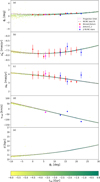 |
Fig. A.1. As Fig. 10, but for the same GC progenitor on the best-fit orbit from Sec. 3.1. No significant differences are seen between the track of the orbit and that defined by the stream stellar particles in the N-body simulation. |
Appendix B: Neglecting the LMC
To ensure that the LMC can be neglected as a cause of substructure, we studied the time variation of the ratio between the forces from Sgr and the LMC on Jhelum, and compared this to the force of the MW on Jhelum to put this in context. This is shown in Fig. B.1 for Simulation 2. This behaviour is qualitatively similar for all four simulations discussed in Sect. 4.4.
We calculated the force from Sgr on Jhelum from Simulation 2, using the time-varying model for Sagittarius from Appendix C. The force from the MW on Jhelum was calculated using AGAMA. Forces from the LMC were calculated with respect to the orbit of the LMC, which we find using galpy’s implementation of the Chandrasekhar dynamical friction force (Bovy 2015) in the Price-Whelan potential. To determine the scale radius of the LMC we followed Erkal et al. (2019), and assuming the present-day mass of the LMC of 1.4 × 10¹¹M⊙ and a Plummer profile this gives rs = 4.8 kpc and hence a half-mass radius of rhm ∼ 6.3 kpc.
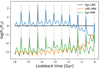 |
Fig. B.1. Logarithm of the ratio between forces of Sgr, the LMC and the MW on Jhelum through time for Simulation 2. The blue line shows the ratio between the forces from the LMC and Sgr on Jhelum. The orange (green) line shows the ratio between the force from the LMC (Sgr) and the MW. The vertical dashed lines show minima in the distance between Jhelum and Sgr, with the red dashed vertical lines showing the closest, most impactful interactions from Table 3. The black horizontal line shows where the forces are equal. |
We see that the ratio FSgr/FLMC varies between 0.5 − 300 before ∼1 Gyr, with maxima at close interactions between Jhelum and Sgr. We note that during the period before ∼1 Gyr the force from the LMC compared to the MW is negligible (a ratio of ∼10−3), meaning that even when FSgr/FLMC < 1, the effect of the LMC can be neglected. On the other hand, Sgr’s force reaches up to ∼50% of the MW’s force multiple times, specifically at close interactions between Jhelum and Sgr. At these close interactions, Sgr causes a large force gradient along the Jhelum stream which causes the final substructure.
As the LMC is at first infall, the closest passage between Jhelum and the LMC is approximately at present day. Figure B.1 shows that the LMC’s force increased to up to 10% of the MW’s force during the past ∼1 Gyr. The close passage with the LMC causes a force gradient of up to ∼10% along the Jhelum stream (see also Shipp et al. (2021)). However, this force gradient will not cause visible substructure due to the time needed for the system to react.
Appendix C: A time-varying model of Sgr
To model a time-varying Sagittarius we followed the procedure outlined in Sect. 4.2. We set out to model Sgr as one particle with a mass and softening scale that vary with time in our simulations of the interactions with Jhelum using GADGET-4. This can be done by assuming a Plummer potential for Sgr of which the mass and scale radius parameters represent the mass and softening scale of the simulated particle.
To parameterize the evolution of the progenitor of Sgr as it disrupts in a MW-like potential, we fitted a Plummer model to the bound particles in each snapshot of the N-body simulation of Sgr (see Sect. 4.2 for details). The time evolution of the fitted scale radius and mass can be seen in Fig. C.1 as dotted lines. Although a Plummer model does not perfectly fit the distribution of bound stars as Sgr orbits around the MW, the deviation is at most 7% in the mass profile.
After determining the values of the characteristic parameters in each snasphot, we fitted a smooth polynomial model to describe their evolution in time. This is shown by the solid lines in Fig. C.1. This approximation is very good as the deviations in the mass profile are up to ∼1%.
Therefore, this method of modelling a time-varying Sgr is acceptable for our general purposes of modelling the impact of a mass-varying satellite on a stellar stream.
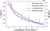 |
Fig. C.1. The smooth polynomial fit to the parameters of the Plummer model fitted to the disrupting Sgr progenitor over time. The dashed lines show the behaviour of the parameters of the Plummer fit to Sgr through the simulations. The solid lines show the smooth polynomials fitted to this behaviour. |
All Tables
Sampling parameters for the initial conditions of the orbit integrations of Jhelum and the parameters of the four selected orbits used for the N-body experiments integrated with GADGET-4. For these integrations, α and δ were kept at a fixed value.
All Figures
|
Fig. 1. Top panel: Hess diagram of stars selected in reflex corrected PM space following Bonaca et al. (2019b), and with |ϕ2|< 2 deg and RUWE < 1.4. The diagram has been smoothed using a 0.4 mag Gaussian kernel. The dashed line shows the selection from the same authors, while the solid line shows that adopted in this work. Our selection is based on a 12 Gyr, [Fe/H] = −1.7 PARSEC isochrone at a distance of 13 kpc. The red circles show confirmed stream members from Ji et al. (2020). Bottom panel: reflex corrected PM for stars selected according to the CMD mask shown above. Jhelum candidates are coloured coded by their membership probability. |
| In the text | |
|
Fig. 2. Positions in (ϕ1, ϕ2) of stars with a membership probability larger than 50% and parallax < 0.8 mas displayed as a scatter plot (top) and a smoothed density map (bottom). Jhelum clearly stands out as an overdensity and has a clumpy morphology with multiple gaps. Possible narrow-component members are contained within the red region in the top panel. Below this region, the extended broad component stands out, while above it, between ϕ1 ≈ 0–5 degrees, a thus far unreported third component can be seen. |
| In the text | |
|
Fig. 3. Stars with a membership probability larger than 50%, parallax < 0.8 mas and 5 ≤ ϕ1/deg ≤ 25, −3 ≤ ϕ2/deg ≤ 3 are shown as black dots in (panel a) on the sky (ϕ1, ϕ2), in (b) in (ϕ1, |
| In the text | |
|
Fig. 4. Distribution of high probability narrow component members (> 50%) in (a), (ϕ1, ϕ2), (b), (ϕ1, |
| In the text | |
|
Fig. 5. Posterior parameter distribution of the initial conditions of the best-fit orbit of Jhelum for σnuis = 6.7 km s−1 in the default MW potential. We note the (expected) strong degeneracy between the distance and μδ. |
| In the text | |
|
Fig. 6. Best-fit single orbit of Jhelum in the default MW potential for σnuis = 6.7 km s−1 (dark blue line) and σnuis = 2 km s−1 (dashed light orange line). 100 orbits were sampled randomly from the MCMC chains for the higher and lower values of σnuis, and are shown in light indigo and in orange respectively. The binned estimates and their 1σ uncertainties are plotted in red, while the individual RV-NC-stars (along with their names) are plotted in blue for σnuis = 6.7 km s−1 (and light-blue for its smaller value). Though the orbits follow the binned track and RV-NC-stars well within the error bars in position and PM, in radial velocity no orbits go through all of the four RV-NC stars: Jhelum2_14 and especially Jhelum1_5 lie far outside the sampled range in radial velocity. The distance to the stream is somewhat low in comparison to the estimate by Shipp et al. (2018), but consistent with the estimate by Li et al. (2022). |
| In the text | |
|
Fig. 7. Posterior parameter distribution of the initial conditions of Jhelum’s best-fit orbit and of the parameters of the Galactic halo potential, for σnuis = 6.7 km s−1. We note that here, the bulge and disk were kept fixed and set to be those of the default MW potential. The posterior parameter distribution of the initial conditions resembles the one of the default MW potential shown in Fig. 5. There is a strong degeneracy between Mh and rs, as expected, and is a result of the circular velocity constraint. The correlation between qx and qz is set by the requirement that the halo density be positive. |
| In the text | |
|
Fig. 8. Best-fit single orbit of Jhelum for the default MW potential (dark blue line) and the MW potential with triaxial halo (dashed light green line) for σnuis = 6.7 km s−1. 100 orbits sampled randomly from the MCMC chains are shown using the same colour as the corresponding best-fit orbits. We note that allowing parameters of the Galactic potential to vary given the constraints does not yield significantly different orbits. |
| In the text | |
|
Fig. 9. Best-fit orbit of Jhelum in the default MW potential (for σnuis = 6.7 km s−1) plotted together with the orbit of Sgr (using the coordinates of M 54, see Table 1), both integrated backwards in time for 6 Gyr. The arrows indicate the direction in which Jhelum and Sgr are currently moving. It is clear that Jhelum and Sgr share approximately the same orbital plane, which results in repeated close encounters between the two. We note that Jhelum is currently passing through pericenter, which is the reason for the high observed velocity gradient seen in Fig. 8. |
| In the text | |
|
Fig. 10. Simulation 1 of the Jhelum stream after interacting with the Sgr dwarf spheroidal. The individual star particles from Jhelum are colour-coded according to the lookback time at which they became unbound. Panel a: shows the stream in ϕ1-ϕ2 frame, while (panels b) and (c) show the (non-reflex corrected) PM in the ϕ1 and ϕ2 directions respectively. Panel d: radial velocity, and Panel (e) the distance. The red datapoints correspond to the binned Jhelum data from Sect. 2.2, and the blue datapoints correspond to stars from Ji et al. (2020) that are likely members of the narrow component of Jhelum. The magenta triangle corresponds to Jhelum2_2, the datapoint which in our simulations marks the present-day location of the progenitor. The magenta dotted line shows the trajectory of the centre of mass of the Jhelum progenitor, and the grey dashed line shows the result from the MCMC best-fit with σnuis = 6.7 km s−1 from Sect. 3.1. Panel a: clear secondary and tertiary components, which are also apparent in the other panels. These additional components are made up of particles that were released early on in the formation of the stream. |
| In the text | |
|
Fig. 11. As Fig. 10, but now for Simulation 2. The bottom component is short, dense and close to the narrow component. To the left, the leading tail shows signs of a diffuse tertiary component that is the result of a ‘folding’. |
| In the text | |
|
Fig. 12. As Fig. 10, but now for initial conditions 3. The trailing tail has completely folded over and shows up as the component on top of the narrow component, and the leading tail shows up as a tertiary component to the bottom of the narrow component on the left of the figure. The two additional components are clearly visible in μϕ2. |
| In the text | |
|
Fig. 13. As Fig. 10, but now for initial conditions 4. Here in Panel (a) we see a more diffuse secondary component in the bottom, and a tertiary component in the top, see for comparison to Figs. 10–12. This stream also has a very clear separation of the components in vrad, even fitting Jhelum1_5. |
| In the text | |
|
Fig. 14. Possible narrow component members in (ϕ1, ϕ2). The binned track with 1σ uncertainty range are indicated in red. The polynomial fitted to this track, Eq. (8), is shown in orange. For comparison, the Bonaca et al. (2019b) median is overplotted in green. The updated polynomial fit seems to follow the narrow component more closely. |
| In the text | |
|
Fig. A.1. As Fig. 10, but for the same GC progenitor on the best-fit orbit from Sec. 3.1. No significant differences are seen between the track of the orbit and that defined by the stream stellar particles in the N-body simulation. |
| In the text | |
|
Fig. B.1. Logarithm of the ratio between forces of Sgr, the LMC and the MW on Jhelum through time for Simulation 2. The blue line shows the ratio between the forces from the LMC and Sgr on Jhelum. The orange (green) line shows the ratio between the force from the LMC (Sgr) and the MW. The vertical dashed lines show minima in the distance between Jhelum and Sgr, with the red dashed vertical lines showing the closest, most impactful interactions from Table 3. The black horizontal line shows where the forces are equal. |
| In the text | |
|
Fig. C.1. The smooth polynomial fit to the parameters of the Plummer model fitted to the disrupting Sgr progenitor over time. The dashed lines show the behaviour of the parameters of the Plummer fit to Sgr through the simulations. The solid lines show the smooth polynomials fitted to this behaviour. |
| In the text | |
Current usage metrics show cumulative count of Article Views (full-text article views including HTML views, PDF and ePub downloads, according to the available data) and Abstracts Views on Vision4Press platform.
Data correspond to usage on the plateform after 2015. The current usage metrics is available 48-96 hours after online publication and is updated daily on week days.
Initial download of the metrics may take a while.