| Issue |
A&A
Volume 660, April 2022
|
|
|---|---|---|
| Article Number | L8 | |
| Number of page(s) | 9 | |
| Section | Letters to the Editor | |
| DOI | https://doi.org/10.1051/0004-6361/202142478 | |
| Published online | 12 April 2022 | |
Letter to the Editor
Bipolar planetary nebulae from common-envelope evolution of binary stars⋆
1
Max Planck Institute for Solar System Research, Justus-von-Liebig-Weg 3, 37077 Göttingen, Germany
e-mail: This email address is being protected from spambots. You need JavaScript enabled to view it.
2
Zentrum für Astronomie der Universität Heidelberg, Institut für Theoretische Astrophysik, Philosophenweg 12, 69120 Heidelberg, Germany
3
Heidelberger Institut für Theoretische Studien, Schloss-Wolfsbrunnenweg 35, 69118 Heidelberg, Germany
4
Zentrum für Astronomie der Universität Heidelberg, Astronomisches Rechen-Institut, Mönchhofstr. 12-14, 69120 Heidelberg, Germany
5
Max Planck Institute for Astronomy, Königstuhl 17, 69117 Heidelberg, Germany
6
Max Planck Computing and Data Facility, Gießenbachstraße 2, 85748 Garching, Germany
7
Max Planck Institute for Astrophysics, Karl-Schwarzschild-Str. 1, 85748 Garching, Germany
Received:
19
October
2021
Accepted:
23
February
2022
Abstract
Asymmetric shapes and evidence for binary central stars suggest a common-envelope origin for many bipolar planetary nebulae. The bipolar components of the nebulae are observed to expand faster than the rest, and the more slowly expanding material has been associated with the bulk of the envelope ejected during the common-envelope phase of a stellar binary system. Common-envelope evolution in general remains one of the biggest uncertainties in binary star evolution, and the origin of the fast outflow has not been explained satisfactorily. We perform three-dimensional magnetohydrodynamic simulations of common-envelope interaction with the moving-mesh code AREPO. Starting from the plunge-in of the companion into the envelope of an asymptotic-giant-branch star and covering hundreds of orbits of the binary star system, we are able to follow the evolution to complete envelope ejection. We find that magnetic fields are strongly amplified in two consecutive episodes: first, when the companion spirals in the envelope and, second, when it forms a contact binary with the core of the former giant star. In the second episode, a magnetically driven, high-velocity outflow of gas is launched self-consistently in our simulations. The outflow is bipolar, and the gas is additionally collimated by the ejected common envelope. The resulting structure reproduces typical morphologies and velocities observed in young planetary nebulae. We propose that the magnetic driving mechanism is a universal consequence of common-envelope interaction that is responsible for a substantial fraction of observed planetary nebulae. Such a mechanism likely also exists in the common-envelope phase of other binary stars that lead to the formation of Type Ia supernovae, X-ray binaries, and gravitational-wave merger events.
Key words: planetary nebulae: general / binaries: general / stars: winds, outflows / stars: magnetic field / stars: AGB and post-AGB / magnetohydrodynamics (MHD)
Movies associated with Figs. A.1–A.3 are available at https://www.aanda.org
© P. A. Ondratschek et al. 2022
 Open Access article, published by EDP Sciences, under the terms of the Creative Commons Attribution License (https://creativecommons.org/licenses/by/4.0), which permits unrestricted use, distribution, and reproduction in any medium, provided the original work is properly cited.
Open Access funding provided by Max Planck Society.
1. Introduction
Planetary nebulae (PNe) are iconic astronomical objects where the hot core of a former giant star illuminates expelled envelope material. They not only highlight spectacular mass loss episodes in stellar evolution, but they are also instrumental as standard candles in the cosmic distance ladder (Roth et al. 2021). In 80%–85% of cases, the nebulae are asymmetric, with pronounced bipolar shapes, and some show jet-like features (Sahai & Trauger 1998; Parker et al. 2006). Yet, the mechanism driving these bipolar, jet-like outflows remains elusive. The central stars of at least 15% of PNe (Miszalski et al. 2009) are known to be close binary systems, but the true binary fraction is much higher, probably exceeding 60% (De Marco et al. 2015; Boffin & Jones 2019). This suggests that at least a large fraction of PNe originates from common-envelope (CE) interaction in binary stellar systems, where a star spirals into the envelope of a giant and eventually ejects it (Paczynski 1976; Nordhaus & Blackman 2006; De Marco 2009; Boffin & Jones 2019).
Bipolar PNe are often observed to consist of two main components (Sahai & Trauger 1998): a toroidal structure of slowly expanding gas (≈20 km s−1) and a perpendicular, fast bipolar (sometimes jet-like) outflow (≈70 km s−1, in many cases exceeding 100 km s−1; see Imai et al. 2002; Tafoya et al. 2020; Guerrero et al. 2020). Magnetic fields have been inferred in such bipolar outflows, for example from synchrotron emission (Perez-Sanchez et al. 2013), dust continuum polarization (Sabin et al. 2015), and maser emission (Miranda et al. 2001), and are thought to help collimate them (Vlemmings et al. 2006). The low-velocity component has been associated with the CE of a binary stellar system that is ejected preferentially into the region around its orbital plane. Its approximate rotational symmetry with a polar cavity forms a nozzle for a later fast outflow that is driven by an as yet unknown mechanism. Ad hoc central engines have been applied in toy models of post-CE systems and demonstrate that such models can indeed reproduce a wide variety of features found in PNe. Suggested engines include enhanced radiation-driven winds (spherically symmetric as well as bipolar; Morris 1981; García-Segura et al. 2005; Zou et al. 2020), magnetically driven winds (García-Segura et al. 2020), and jets launched from a circumbinary disk (Soker & Livio 1994; Garcia-Segura et al. 2021).
Here, we explore the mechanism that forms bipolar PNe in the CE interaction of binary systems using detailed and self-consistent magnetohydrodynamic (MHD) simulations. We briefly describe our simulations in Sect. 2, present our main findings in Sect. 3, and conclude in Sect. 4.
2. Methods
Our simulations were performed in three steps, closely following earlier work (Ohlmann et al. 2016a, 2016b; Kramer et al. 2020; Sand et al. 2020). First, we evolved a 1.2 M⊙ zero-age main-sequence star at solar metallicity with the one-dimensional stellar evolution code MESA (Paxton et al. 2011, 2013, 2015) in version 7624. We used the default MESA settings and accounted for stellar wind mass loss via the Reimers (1975) prescription with the wind scaling factor η = 0.5 for red giant stars and via the Blöcker (1995) prescription with η = 0.1 for asymptotic-giant-branch (AGB) stars. For the CE simulations presented here, we constructed an early AGB model that has a mass of Mprim = 0.970 M⊙ and a radius of 173 R⊙ by the time the CE interaction commences. Following the procedure of Ohlmann et al. (2017), we replaced the 0.545 M⊙ core of this stellar model with a point particle that interacts only gravitationally with the gas of the envelope.
Second, we mapped the primary star into the MHD moving-mesh code AREPO (Springel 2010; Pakmor et al. 2011; Pakmor & Springel 2013) and performed a relaxation as described by Ohlmann et al. (2017) to reestablish hydrostatic equilibrium in the envelope. Both the relaxation step and the subsequent CE simulations use the OPAL equation of state (Rogers et al. 1996; Rogers & Nayfonov 2002). The overall relaxation was carried out for ten dynamical timescales of the primary star, half of the time damping spurious velocities and the other half ensuring a hydrostatically stable model. At the end of the relaxation, the star had been resolved by about 5 million cells.
Third, we added a Mcomp = 0.243 M⊙ companion, which could be a white-dwarf or a main-sequence star, at a distance of 207 R⊙ from the center of the primary star. The mass ratio between the companion and the primary star in this reference simulation was q = 0.25. To explore the effect of varying mass ratios, two additional setups were used, with q = 0.5 (Mcomp = 0.486 M⊙, placed at a distance of 236 R⊙) and q = 0.75 (Mcomp = 0.729 M⊙, initial distance 256 R⊙). In all our simulations, the companion was unresolved and represented by a point particle in the same way as the core of the primary star. The stellar envelope was initially set to solid-body rotation at 95% of the orbital velocity of the binary system. We employed adaptive mesh refinement to ensure high resolution around both point particles.
Our setup parameters were the same as those of Sand et al. (2020), except for a seed magnetic dipole field that we added to the primary star’s envelope in our reference simulation labeled “MHD.” As a comparison, one simulation (labeled “non-MHD”) was performed with identical parameters but no initial magnetic field. The initial polar surface field strength was set to 10−10 G, similar to the models of Ohlmann et al. (2016b). Using the OPAL equation of state in all our simulations, we followed changes in the ionization state of the gas caused by the expansion of the stellar envelope. In our model, released recombination energy is assumed to thermalize locally. If converted into kinetic energy, it can support envelope ejection.
3. Results
3.1. Dynamical evolution during the common-envelope phase
After the companion is placed at a distance of 207 R⊙ from the center of the primary star (Figs. 1a,f), it is immediately dragged into the envelope of the giant (see also the videos in Figs. A.1 and A.2). The core of the primary star and the companion orbit each other inside a CE, causing a spiral density structure (Fig. 1b).
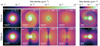 |
Fig. 1. Density evolution during the CE phase in our reference simulation. The panels are slices of gas density in the face-on view (top row) and edge-on view (bottom row). The cross symbol indicates the position of the core of the giant star and the plus symbol that of the companion. Panels e, j: zoomed-in views of the central region indicated by the gray boxes in panels c and h, respectively. The actual simulation domain is much larger than the panels shown here. Roche equipotential lines and the positions of the Lagrange points are added in panel e. |
Drag forces on the companion and on the core of the giant transfer angular momentum and energy to the envelope gas, leading to orbital decay. In Fig. 2 we compare the orbital separation between the core of the AGB star and the companion in our reference MHD case and its corresponding non-MHD version. In both simulations, the orbital separations decrease similarly, from 207 R⊙ to 21.5 R⊙ (non-MHD) and 21.0 R⊙ (MHD). The final orbital periods of the systems are 13.1 d (non-MHD) and 12.6 d (MHD). By the time the MHD simulation is stopped, only 1.65 × 10⁻⁴ M⊙ of gas remains in the vicinity of the cores. The generated magnetic-field energy (Emag ≈ 1043 erg; see Sect. 3.2) is smaller by a factor of 1000 than the kinetic and potential energies of the cores and the envelope (≈1046 erg). Hence, magnetic fields do not influence the final orbital separation of the system significantly. The dynamical plunge-in ends when the orbital decay slows down at ∼1000 d (∼25 orbits; see Fig. 2), and the spiral structure is washed out by the many orbits of the remnant binary around the common center of mass (Fig. 1c).
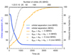 |
Fig. 2. Evolution of orbital separation and unbound mass fraction of the envelope in the simulations, taking magnetic fields into account (MHD) and neglecting magnetic fields (non-MHD). In both simulations, MHD and non-MHD, local thermalization of released recombination energy is assumed. For the non-MHD simulation, we show only data until t = 3568 d. The unbound mass fraction is computed according to a kinetic-energy criterion (orange) and an internal-energy criterion, which additionally includes ionization energy released in recombination processes (gray). |
We used two criteria to measure the fraction of unbound to total envelope mass: A lower limit to the unbound mass is given by the “kinetic-energy criterion”, which includes only the kinetic, ekin, and the potential energy, egrav, of each gas cell (orange lines in Fig. 2). According to this criterion, mass is unbound if egrav+ ekin > 0. The “internal-energy criterion”, egrav + ekin + eint > 0 (gray lines in Fig. 2), additionally includes the thermal and ionization energy of the gas cells, eint, and provides an upper limit. The contribution of magnetic-field energy is negligible. There is almost no difference in the unbound mass fractions as given by the internal-energy criterion between the MHD and the non-MHD simulations. Applying the kinetic-energy criterion, we find a slightly faster mass unbinding in the MHD simulation. Nevertheless, the unbound mass fractions converge to very similar values in both cases. Almost the entire envelope is unbound as measured by the kinetic-energy criterion (99.4% MHD and 98.8% non-MHD). The success of almost complete envelope ejection is therefore independent of magnetic fields and is mainly due to including recombination energy in the simulations.
Here, the released recombination energy is assumed to thermalize locally. This appears to be a reasonable assumption because most of the recombination of hydrogen takes place inside a volume enclosed by the photosphere (see Fig. B.1). In addition, helium recombines close to the center of the envelope in optically thick regions (Fig. B.1). While this justifies our assumption of local thermalization of the recombination energy within our simulation, it does not prove that photon diffusion and radiative losses are completely negligible. Our models can be viewed as an upper limit to envelope ejection. Sand et al. (2020) present a simulation for the same setup without magnetic fields that neglects ionization energy in the equation of state. They indeed find that only about 16% of the envelope is ejected, which can be considered as a lower limit. Given that most of the recombination is found to occur inside the optically thick part of the envelope, we consider almost full envelope ejection the more likely outcome for the binary system studied here. Ultimately, however, this has to be confirmed with models that account for potential losses of recombination energy by radiation.
In order to compare the binding energy of the envelope of the primary star, Ebin, to the orbital energy released during the inspiral process, ΔEorb, we computed the CE ejection efficiency, αCE = Ebin/ΔEorb. Here, Ebin and ΔEorb are defined as in Sand et al. (2020), and we consider the two cases in which (i) only gravitational energy (αCE, g) and (ii) gravitational plus internal energy (αCE, b) are taken into account in the computation of Ebin. In our reference simulation we obtain αCE, g = 2.87 and αCE, b = 0.32 at the time when the calculation is terminated. Our values are in good agreement with those found in Sand et al. (2020) and differ only slightly because our new MHD simulations are evolved longer until almost full envelope ejection is reached.
During the plunge-in of the companion, the now centrifugally supported envelope starts to expand into a toroidal structure in the orbital plane with low density funnels around the polar axis (Figs. 1b,g). While the envelope expands, gas with low specific angular momentum falls back onto the central binary along the orbital angular-momentum vector. This transforms the funnels into a narrow, low-density chimney (Fig. 1h).
Shortly after 1000 d, the envelope is virtually unbound according the internal-energy criterion. This, however, is not the end of the dynamical interaction. At about this time, a contact phase sets in between the companion and the former core of the giant star (Figs. 1e,j) where both stars overfill their respective Roche lobes as indicated by the Roche potential in Fig. 1e. At ∼1500 d, we observe a new and important feature in our CE simulation: a high-velocity outflow (90−130 km s−1) emerges perpendicular to the orbital plane from the region of the central core binary. This is visible in the density structure (Fig. 1i) but is clearer in the radial velocity component shown in Fig. 3a. The outflow builds up gradually, is first launched into one hemisphere only, and then precesses. Once fully established, it becomes bipolar and is collimated along the chimney-like underdensity, which is embedded in the remainder of the CE. By the time it launches, at least 70% of the envelope of the former giant star has been ejected. Our non-MHD comparison simulation undergoes a nearly identical evolution, resulting in similar envelope mass ejections, but it develops no fast polar outflow. Instead, it shows an almost spherical expansion of the envelope, with only minor angular variations in the velocity (Fig. 3b). Together with the fact that the magnetic pressure in the outflowing material is higher than the thermal pressure (Fig. 5j), this implies that the outflow is magnetically driven. It is thus an inevitable consequence of the magnetic-field amplification that we observe in our CE simulation.
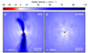 |
Fig. 3. Radial velocity in the MHD reference simulation (a) and the non-MHD simulation (b) plotted edge-on. |
3.2. Amplification of magnetic fields
During the plunge-in, the total magnetic energy in the envelope increases exponentially by more than 15 orders of magnitude (Fig. 4a). The strongest amplification of the magnetic field is observed in the region around the companion star (Fig. 4d), which accretes about 10−5 M⊙ while moving through the envelope, and in a shear layer between the spiral arm emerging at the companion and the rest of the envelope. We identify three mechanisms of magnetic-field amplification.
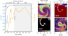 |
Fig. 4. Amplification of magnetic fields. In panel a, the total magnetic energy is shown as a function of time on a logarithmic scale (blue) and on a linear scale (orange). Panels b, c, d, e: the sonic Mach number, the ratio of the wavelength of the fastest growing MRI mode and the AREPO cell size (λMRI/lcell), and the absolute magnetic-field strength (|B|) in the orbital plane, respectively. They provide details of the two episodes of field amplification: at t = 352 d, marked with black dots, and at t = 1504 d, indicated with red dots. |
The first is the magneto-rotational instability (MRI; Balbus & Hawley 1991), which acts close to the companion and near the core of the giant star. A comparison of the wavelength of the fastest growing mode to the size of the AREPO grid cells demonstrates that the MRI is well resolved in these regions (Fig. 4c). The e-folding growth time of the magnetic energy in our simulation is about 8 d, which is on the order of the expected MRI growth time1 of ≈15–20 d.
The second are Kelvin-Helmholtz instabilities, which occur in shear layers that are visible in Mach number (Fig. 4b) in combination with the MRI. The amplified field is seen in the region trailing the companion (marked by the plus symbol in Fig. 4d).
The third are convective fluid motions as in dynamo processes. They create an isentropic region around the core of the primary (Fig. 4d, region around the cross symbol).
The MRI amplifies the magnetic field close to the positions of the core of the primary and the companion. Within a sphere of radius r = 8.7 R⊙ around the point particles, the gravitational potential is softened using a spline function. The artificially softened gravitational potential reduces the gradients of the flow velocities, which implies the amplification processes tend to be underestimated.
After the initial fast orbital decay, at ∼1000 d, the magnetic-field energy reaches a maximum of about 1043 erg. This terminates the first phase of magnetic-field amplification (Fig. 4a). The magnetic flux is conserved in ideal MHD, which causes a decrease in the magnetic-field energy when the envelope starts to expand significantly (Fig. 4a, between 1000 d − 1300 d). This decrease is reversed at ≳1300 d (i.e., at about the time when the magnetically driven outflow emerges) because gas flows that establish when the core binary enters a contact phase lead to further magnetic-field amplification (Fig. 4e). This amplification is driven by shear layers in the gas streams subject to the MRI, similar to the situation in the merger of two main-sequence stars (Schneider et al. 2019). In the amplification region, the wavelength of the fastest growing MRI mode is larger by a factor of 10 to 100 than the typical cell size. In the Roche-lobe-overflow material, the magnetic-field energy grows to a similar order of magnitude as the total kinetic energy of the gas, leading to equipartition values of Emag/Ekin ≈ 1. In some regions, even super-equipartition is reached. This is known from fast-rotating systems (e.g., Augustson et al. 2016) and indicates dynamo action in conjunction with the MRI. The mass exchange in the core binary is nonconservative, and highly magnetized material is lost through the outer Lagrangian points. This continued magnetic-field amplification in the contact binary eventually launches the high-velocity outflow parallel to its axis of rotation (see video in Fig. A.3).
3.3. Launching of the outflow
The complex flows close to the core binary system (e.g., Figs. 1e,j) do not reproduce the idealized picture of an accretion or circumbinary disk often associated with the launching of magnetized outflows. Still, the global symmetry and the motion of the stellar cores in the orbital plane create a strong, preferentially poloidal magnetic field along the chimney that has a diameter of about the binary’s orbital separation (Fig. 5h). The outflowing material is accelerated to velocities of 90−130 km s−1 (Fig. 5f), approximately matching the ∼85 km s−1 orbital velocity of the core binary. The material in the outflow corotates at a lower speed of about ∼40 km s−1.
 |
Fig. 5. Evolution and launching of the bipolar outflow perpendicular to the orbital plane. The gas density in panels a–d traces the evolution of the outflow, and in panel e we show the absolute magnetic field at the same time as in panel d. The bottom panelsf–m (rotated by 90° with respect to the upper panels), are at a time of 2880 d and illustrate the launching of the outflow. Shown are the radial velocity vrad (f, g), the ratio of poloidal to toroidal magnetic-field strength Bpol/Btor (i, h), the ratio of magnetic to thermal pressure β−1 (j, k), and the poloidal Alfvén Mach number |
The flow structure in the acceleration region is characterized by a small poloidal Alfvén Mach number, MA = 10−2 < 1 (Fig. 5l). This is a typical signature of a magneto-centrifugally driven outflow launched by the Blandford–Payne mechanism (Blandford & Payne 1982). In Figs. 5k,l, we indicate the “force-free” regions where both β−1 = Pmag/Pgas > 1 and MA < 1. In these regions, the magnetic pressure exceeds the thermal and the dynamic pressure, and fluid elements can therefore be accelerated along the magnetic-field lines by centrifugal forces. Additionally, a magnetic pressure gradient of the poloidal field contributes to the acceleration of material.
In the circumbinary envelope material, however, the magnetic field is dominated by its toroidal component, which results from strong differential rotation (Fig. 5i). It contributes to the overall acceleration of the bipolar outflow – an effect similar to magnetic tower jets (Uchida & Shibata 1985; Lynden-Bell & Boily 1994) that, for example, arise during star formation (e.g., Pudritz & Ray 2019). The outflow is replenished by the accretion of leftover envelope material in the orbital plane, as indicated by the negative radial velocity in Fig. 5g. As the high-velocity outflow propagates along the collimating chimney inside a higher-density cocoon (Figs. 5b–d), its interaction with the expanding envelope material creates bow shocks with sonic Mach numbers of 2–3.
3.4. Sensitivity to mass ratio
To explore the universality of the mechanism that produces high-velocity outflows, we carried out two additional MHD simulations with initial mass ratios of q = 0.5 and q = 0.75. In the case of q = 0.50, the orbit shrinks to a final separation of 37.8 R⊙, corresponding to a period of 26.9 d. For q = 0.75, the remaining stars are separated by 54.2 R⊙ (orbital period: 65.8 d) by the time the computation is stopped. The distance between the two stars is still decreasing slightly at the end of all simulations. During the simulated time, the model with mass ratio q = 0.50 (q = 0.75) unbinds at least 99.8% (97.0%) of the gas mass according to the kinetic-energy criterion.
As can be seen in Fig. 6, pronounced bipolar outflows are launched in all simulations regardless of the initial mass ratio of the binary. We observe different maximum outflow velocities. In the models with mass ratios q = 0.25 and q = 0.50, radial velocities of > 120 km s−1 dominate the outflow, whereas in the simulation with the largest companion mass (q = 0.75) the fastest velocities are on the order of 60−70 km s−1. It is possible that the strength of the outflow in the latter simulation will further increase. However, as discussed in Sect. 3.3, the outflow velocities are related to the orbital velocities of the remnant binary. Given the tighter orbits reached in simulations with lower-mass companions, we indeed expect faster outflows in such cases, as indicated in Fig. 6.
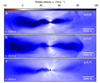 |
Fig. 6. Radial velocities in simulations with different mass ratios, q, of companion and primary-star mass, as indicated. |
3.5. Comparison to observations
The bipolar outflow and the structure of the ejected envelope define the morphology of the forming PN. To compare the obtained outflow structure with observations, we show a three-dimensional rendering of our model at 4400 d and a Hubble Space Telescope image of the protoplanetary Calabash Nebula (OH 231.8+04.2) in Fig. 7. Our model is neither meant to reproduce this particular nebula quantitatively nor does it predict the observables directly, but the morphological similarities are striking. A lopsided bipolar, jet-like outflow is launched from a central toroidal structure inside which a binary central star is present. It terminates in bow shocks on both ends, visible as high temperatures at the top and bottom of the bipolar outflow (Fig. 7). The high temperature region at the waist of the structure originates from the circumbinary material around the central contact binary.
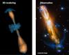 |
Fig. 7. Qualitative morphological comparison between the simulated outflow and observations of the Calabash Nebula (OH 231.84 +4.22). Left panel: geometry of the outflow represented by radial velocity (orange) and temperature (blue). Right panel: composite, optical image taken by the NASA/ESA Hubble Space Telescope. We note that the rendering of our simulation is not to scale with the observation. |
The bipolar outflow of the Calabash Nebula is known to be threaded by an ordered magnetic field (Leal-Ferreira et al. 2012; Sabin et al. 2015), which further supports our model (Fig. 5e). The expansion velocity of our toroidal structure of order 10−30 km s−1 (Fig. 5f) and the 90−130 km s−1 bipolar outflow are broadly consistent with observations of young (proto-)PNe and post-AGB stars (Imai et al. 2002; Tafoya et al. 2020; Guerrero et al. 2020). In our simulation, we measure mass outflow rates of Ṁ ≃ 10−5−10−3 M⊙ yr−1, which is consistent with observational findings (Lorenzo et al. 2021). This shows that our proposed mechanism self-consistently reproduces the structures observed in such systems.
4. Discussion and conclusions
In analogy to the robustness against variations in the mass ratio of the system, we expect that the same mechanism operates in CE phases of primary stars with different masses. The morphology of the ejected CE material depends on the initial parameters of the system, and some simulations show less pronounced chimney structures (Ohlmann et al. 2016a), which offers an explanation for the variety of shapes observed in PNe. We therefore predict that magnetically driven outflows launched by the core binary in late stages of the dynamical CE evolution are responsible for a significant fraction of the observed PNe and post-AGB stars. This is in agreement with results from population synthesis studies (Han et al. 1995).
Orbital separations found in CE simulations are typically too large compared with observations of post-CE systems (Iaconi et al. 2017). In principle, the bipolar outflows found in this study could help alleviate this issue if they persist for longer times after the dynamical CE phase and carry away further angular momentum from the remnant binary. Given the low mass of bound envelope gas remaining in the system by the end of our simulation, however, we expect little impact on the final orbital separation in the case studied here.
Our simulations establish a direct link between some bipolar PNe and the enigmatic CE phase of binary star evolution. Planetary nebulae may thus be promising laboratories to gain further insights into this evolutionary phase, which is also pivotal for the formation of X-ray binaries, Type Ia supernovae, and gravitational-wave sources (Ivanova et al. 2013).
Movies
Movie 1 associated with Fig. A.1 (fig_A1_movie_density_face_on) Access Supplementary Material
Movie 2 associated with Fig. A.2 (fig_A2_movie_density_edge_on) Access Supplementary Material
Movie 3 associated with Fig. A.3 (fig_A3_movie_launching_of_bipolar_outflow) Access Supplementary Material
The MRI wavelength and growth time are computed as in Rembiasz et al. (2016).
Acknowledgments
We thank Giovanni Leidi for discussions about magnetic field amplification processes and the reviewer for useful comments that helped improve our work. This work has received funding from the European Research Council (ERC) under the European Union’s Horizon 2020 research and innovation programme (Grant agreement No. 945806). P.A.O., F.K.R., F.R.N.S., and C.S. acknowledge funding from the Klaus Tschira foundation. This work is supported by the Deutsche Forschungsgemeinschaft (DFG, German Research Foundation) under Germany’s Excellence Strategy EXC 2181/1-390900948 (the Heidelberg STRUCTURES Excellence Cluster).
References
- Augustson, K., Mathis, S., Brun, S., & Toomre, J. 2016, Proc. Int. Astron. Union, 12, 233 [CrossRef] [Google Scholar]
- Balbus, S. A., & Hawley, J. F. 1991, ApJ, 376, 214 [Google Scholar]
- Blandford, R. D., & Payne, D. G. 1982, MNRAS, 199, 883 [CrossRef] [Google Scholar]
- Blöcker, T. 1995, A&A, 297, 727 [NASA ADS] [Google Scholar]
- Boffin, H. M. J., & Jones, D. 2019, The Importance of Binaries in the Formation and Evolution of Planetary Nebulae, SpringerBriefs in Astronomy (Springer Nature Switzerland) [CrossRef] [Google Scholar]
- De Marco, O. 2009, PASP, 121, 316 [NASA ADS] [CrossRef] [Google Scholar]
- De Marco, O., Long, J., Jacoby, G. H., et al. 2015, MNRAS, 448, 3587 [Google Scholar]
- García-Segura, G., López, J. A., & Franco, J. 2005, ApJ, 618, 919 [CrossRef] [Google Scholar]
- García-Segura, G., Taam, R. E., & Ricker, P. M. 2020, ApJ, 893, 150 [CrossRef] [Google Scholar]
- Garcia-Segura, G., Taam, R. E., & Ricker, P. M. 2021, ApJ, 914, 111 [NASA ADS] [CrossRef] [Google Scholar]
- Guerrero, M. A., Suzett Rechy-García, J., & Ortiz, R. 2020, ApJ, 890, 50 [NASA ADS] [CrossRef] [Google Scholar]
- Han, Z., Podsiadlowski, P., & Eggleton, P. P. 1995, MNRAS, 272, 800 [NASA ADS] [Google Scholar]
- Iaconi, R., Reichardt, T., Staff, J., et al. 2017, MNRAS, 464, 4028 [NASA ADS] [CrossRef] [Google Scholar]
- Imai, H., Obara, K., Diamond, P. J., Omodaka, T., & Sasao, T. 2002, Nature, 417, 829 [NASA ADS] [CrossRef] [Google Scholar]
- Ivanova, N., Justham, S., Chen, X., et al. 2013, A&ARv, 21, 59 [Google Scholar]
- Kramer, M., Schneider, F. R. N., Ohlmann, S. T., et al. 2020, A&A, 642, A97 [NASA ADS] [CrossRef] [EDP Sciences] [Google Scholar]
- Leal-Ferreira, M. L., Vlemmings, W. H. T., Diamond, P. J., et al. 2012, A&A, 540, A42 [NASA ADS] [CrossRef] [EDP Sciences] [Google Scholar]
- Lorenzo, M., Teyssier, D., Bujarrabal, V., et al. 2021, A&A, 649, A164 [NASA ADS] [CrossRef] [EDP Sciences] [Google Scholar]
- Lynden-Bell, D., & Boily, C. 1994, MNRAS, 267, 146 [Google Scholar]
- Miranda, L. F., Gómez, Y., Anglada, G., & Torrelles, J. M. 2001, Nature, 414, 284 [NASA ADS] [CrossRef] [Google Scholar]
- Miszalski, B., Acker, A., Parker, Q. A., & Moffat, A. F. J. 2009, A&A, 505, 249 [NASA ADS] [CrossRef] [EDP Sciences] [Google Scholar]
- Morris, M. 1981, ApJ, 249, 572 [NASA ADS] [CrossRef] [Google Scholar]
- Nordhaus, J., & Blackman, E. G. 2006, MNRAS, 370, 2004 [NASA ADS] [CrossRef] [Google Scholar]
- Ohlmann, S. T., Röpke, F. K., Pakmor, R., & Springel, V. 2016a, ApJ, 816, L9 [Google Scholar]
- Ohlmann, S. T., Röpke, F. K., Pakmor, R., Springel, V., & Müller, E. 2016b, MNRAS, 462, L121 [NASA ADS] [CrossRef] [Google Scholar]
- Ohlmann, S. T., Röpke, F. K., Pakmor, R., & Springel, V. 2017, A&A, 599, A5 [NASA ADS] [CrossRef] [EDP Sciences] [Google Scholar]
- Paczynski, B. 1976, in Structure and Evolution of Close Binary Systems, eds. P. Eggleton, S. Mitton, & J. Whelan, IAU Symp., 73, 75 [NASA ADS] [CrossRef] [Google Scholar]
- Pakmor, R., & Springel, V. 2013, MNRAS, 432, 176 [NASA ADS] [CrossRef] [Google Scholar]
- Pakmor, R., Bauer, A., & Springel, V. 2011, MNRAS, 418, 1392 [NASA ADS] [CrossRef] [Google Scholar]
- Parker, Q. A., Acker, A., Frew, D. J., et al. 2006, MNRAS, 373, 79 [NASA ADS] [CrossRef] [Google Scholar]
- Paxton, B., Bildsten, L., Dotter, A., et al. 2011, ApJS, 192, 3 [Google Scholar]
- Paxton, B., Cantiello, M., Arras, P., et al. 2013, ApJS, 208, 4 [Google Scholar]
- Paxton, B., Marchant, P., Schwab, J., et al. 2015, ApJS, 220, 15 [Google Scholar]
- Perez-Sanchez, A. F., Vlemmings, W. H. T., Tafoya, D., & Chapman, J. M. 2013, MNRAS, 436, L79 [NASA ADS] [CrossRef] [Google Scholar]
- Pudritz, R. E., & Ray, T. P. 2019, Front. Astron. Space Sci., 6, 54 [Google Scholar]
- Reimers, D. 1975, Mem. Soc. Roy. Sci. Liege, 8, 369 [Google Scholar]
- Rembiasz, T., Obergaulinger, M., Cerdá-Durán, P., Müller, E., & Aloy, M. A. 2016, MNRAS, 456, 3782 [NASA ADS] [CrossRef] [Google Scholar]
- Rogers, F. J., & Nayfonov, A. 2002, ApJ, 576, 1064 [Google Scholar]
- Rogers, F. J., Swenson, F. J., & Iglesias, C. A. 1996, ApJ, 456, 902 [Google Scholar]
- Roth, M. M., Jacoby, G. H., Ciardullo, R., et al. 2021, ApJ, 916, 21 [NASA ADS] [CrossRef] [Google Scholar]
- Sabin, L., Hull, C. L. H., Plambeck, R. L., et al. 2015, MNRAS, 449, 2368 [NASA ADS] [CrossRef] [Google Scholar]
- Sahai, R., & Trauger, J. T. 1998, AJ, 116, 1357 [NASA ADS] [CrossRef] [Google Scholar]
- Sand, C., Ohlmann, S. T., Schneider, F. R. N., Pakmor, R., & Röpke, F. K. 2020, A&A, 644, A60 [NASA ADS] [CrossRef] [EDP Sciences] [Google Scholar]
- Schneider, F. R. N., Ohlmann, S. T., Podsiadlowski, P., et al. 2019, Nature, 574, 211 [Google Scholar]
- Soker, N., & Livio, M. 1994, ApJ, 421, 219 [NASA ADS] [CrossRef] [Google Scholar]
- Springel, V. 2010, MNRAS, 401, 791 [Google Scholar]
- Tafoya, D., Imai, H., Gómez, J. F., et al. 2020, ApJ, 890, L14 [NASA ADS] [CrossRef] [Google Scholar]
- Uchida, Y., & Shibata, K. 1985, PASJ, 37, 515 [NASA ADS] [Google Scholar]
- Vlemmings, W. H. T., Diamond, P. J., & Imai, H. 2006, Nature, 440, 58 [Google Scholar]
- Zou, Y., Frank, A., Chen, Z., et al. 2020, MNRAS, 497, 2855 [NASA ADS] [CrossRef] [Google Scholar]
Appendix A: Movies of the common-envelope simulation
Figures A.1 and A.2 illustrate the density evolution in the orbital plane and perpendicular to this plane. Figure A.3 shows the launching of the bipolar outflow seen edge-on.
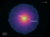 |
Fig. A.1. (Movie online) Movie of density evolution in the orbital plane. Similar to Fig. 1, in this animation the evolution of the density is shown in the orbital plane. |
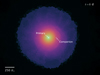 |
Fig. A.2. (Movie online) Movie of density evolution in the plane perpendicular to the orbital plane. Similar to Fig. 1, in this movie the evolution of the density is shown in the plane perpendicular to the orbital plane. |
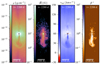 |
Fig. A.3. (Movie online) Movie of the launching of the bipolar outflow. Similar to Fig. 5, we show the evolution of gas density, the absolute magnetic-field strength (|B|), the radial velocity (vrad), and the ratio of magnetic to thermal pressure (β−1) perpendicular to the orbital plane. |
Appendix B: Hydrogen and helium recombination
In Fig. B.1 we show the (still) available ionization-energy density at different epochs in the simulation. The photosphere is determined by radially integrating the optical depth, τ, from outside in until reaching a value of τ = 1. It is illustrated by a gray contour, and the grid cells close to the thus-defined photosphere are already relatively large, precluding a precise localization. The outer edge of the hydrogen recombination front, which we define by a number fraction of ionized hydrogen, xH, of less than 0.2, is located close to the photosphere. However, the inner edge of the hydrogen-recombination region (indicated by xH < 0.9) extends down to the center of the expanding envelope. This shows that energy from recombining hydrogen is mostly released throughout the optically thick region of the envelope and only in minor parts near or outside the photosphere. The outer ionization fronts of HeI and HeII are in even deeper and more opaque layers than those of hydrogen at the center of the envelope.
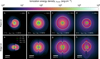 |
Fig. B.1. Ionization-energy density in the reference simulation. The ionization-energy density, ρe, ion, is shown at four different times in the orbital plane (top panels, a–d) and perpendicular to the orbital plane (bottom panels, e–h). The gray contours indicate the approximate position of the photosphere at a given time. As marked in the legend of panel (e), the red and green contours enclose a region where the number fraction of ionized hydrogen is between 0.2 and 0.9 and thus illustrate the region where hydrogen recombines. The purple and blue contours correspond to HeI and HeII number fractions of 0.2, i.e., helium recombines within these layers, close to the center of the expanding envelope. In panels (a)–(d), the current, unbound mass fractions as measured by the kinetic criterion are given (cf. Fig. 2). |
All Figures
|
Fig. 1. Density evolution during the CE phase in our reference simulation. The panels are slices of gas density in the face-on view (top row) and edge-on view (bottom row). The cross symbol indicates the position of the core of the giant star and the plus symbol that of the companion. Panels e, j: zoomed-in views of the central region indicated by the gray boxes in panels c and h, respectively. The actual simulation domain is much larger than the panels shown here. Roche equipotential lines and the positions of the Lagrange points are added in panel e. |
| In the text | |
|
Fig. 2. Evolution of orbital separation and unbound mass fraction of the envelope in the simulations, taking magnetic fields into account (MHD) and neglecting magnetic fields (non-MHD). In both simulations, MHD and non-MHD, local thermalization of released recombination energy is assumed. For the non-MHD simulation, we show only data until t = 3568 d. The unbound mass fraction is computed according to a kinetic-energy criterion (orange) and an internal-energy criterion, which additionally includes ionization energy released in recombination processes (gray). |
| In the text | |
|
Fig. 3. Radial velocity in the MHD reference simulation (a) and the non-MHD simulation (b) plotted edge-on. |
| In the text | |
|
Fig. 4. Amplification of magnetic fields. In panel a, the total magnetic energy is shown as a function of time on a logarithmic scale (blue) and on a linear scale (orange). Panels b, c, d, e: the sonic Mach number, the ratio of the wavelength of the fastest growing MRI mode and the AREPO cell size (λMRI/lcell), and the absolute magnetic-field strength (|B|) in the orbital plane, respectively. They provide details of the two episodes of field amplification: at t = 352 d, marked with black dots, and at t = 1504 d, indicated with red dots. |
| In the text | |
|
Fig. 5. Evolution and launching of the bipolar outflow perpendicular to the orbital plane. The gas density in panels a–d traces the evolution of the outflow, and in panel e we show the absolute magnetic field at the same time as in panel d. The bottom panelsf–m (rotated by 90° with respect to the upper panels), are at a time of 2880 d and illustrate the launching of the outflow. Shown are the radial velocity vrad (f, g), the ratio of poloidal to toroidal magnetic-field strength Bpol/Btor (i, h), the ratio of magnetic to thermal pressure β−1 (j, k), and the poloidal Alfvén Mach number |
| In the text | |
|
Fig. 6. Radial velocities in simulations with different mass ratios, q, of companion and primary-star mass, as indicated. |
| In the text | |
|
Fig. 7. Qualitative morphological comparison between the simulated outflow and observations of the Calabash Nebula (OH 231.84 +4.22). Left panel: geometry of the outflow represented by radial velocity (orange) and temperature (blue). Right panel: composite, optical image taken by the NASA/ESA Hubble Space Telescope. We note that the rendering of our simulation is not to scale with the observation. |
| In the text | |
|
Fig. A.1. (Movie online) Movie of density evolution in the orbital plane. Similar to Fig. 1, in this animation the evolution of the density is shown in the orbital plane. |
| In the text | |
|
Fig. A.2. (Movie online) Movie of density evolution in the plane perpendicular to the orbital plane. Similar to Fig. 1, in this movie the evolution of the density is shown in the plane perpendicular to the orbital plane. |
| In the text | |
|
Fig. A.3. (Movie online) Movie of the launching of the bipolar outflow. Similar to Fig. 5, we show the evolution of gas density, the absolute magnetic-field strength (|B|), the radial velocity (vrad), and the ratio of magnetic to thermal pressure (β−1) perpendicular to the orbital plane. |
| In the text | |
|
Fig. B.1. Ionization-energy density in the reference simulation. The ionization-energy density, ρe, ion, is shown at four different times in the orbital plane (top panels, a–d) and perpendicular to the orbital plane (bottom panels, e–h). The gray contours indicate the approximate position of the photosphere at a given time. As marked in the legend of panel (e), the red and green contours enclose a region where the number fraction of ionized hydrogen is between 0.2 and 0.9 and thus illustrate the region where hydrogen recombines. The purple and blue contours correspond to HeI and HeII number fractions of 0.2, i.e., helium recombines within these layers, close to the center of the expanding envelope. In panels (a)–(d), the current, unbound mass fractions as measured by the kinetic criterion are given (cf. Fig. 2). |
| In the text | |
Current usage metrics show cumulative count of Article Views (full-text article views including HTML views, PDF and ePub downloads, according to the available data) and Abstracts Views on Vision4Press platform.
Data correspond to usage on the plateform after 2015. The current usage metrics is available 48-96 hours after online publication and is updated daily on week days.
Initial download of the metrics may take a while.