| Issue |
A&A
Volume 657, January 2022
|
|
|---|---|---|
| Article Number | A76 | |
| Number of page(s) | 10 | |
| Section | Celestial mechanics and astrometry | |
| DOI | https://doi.org/10.1051/0004-6361/202142055 | |
| Published online | 13 January 2022 | |
Observed tidal evolution of Kleopatra’s outer satellite★
1
Institute of Astronomy, Faculty of Mathematics and Physics, Charles University,
V Holešovičkách 2,
18000
Prague,
Czech Republic
e-mail: This email address is being protected from spambots. You need JavaScript enabled to view it.
2
Université Côte d’Azur, Observatoire de la Côte d’Azur, CNRS,
Laboratoire Lagrange,
France
3
IMCCE, Observatoire de Paris, PSL Research University, CNRS, Sorbonne Universités,
UPMC Univ. Paris 06,
Univ. Lille,
France
4
SETI Institute, Carl Sagan Center,
189 Bernado Avenue,
Mountain View,
CA
94043,
USA
5
Aix Marseille Univ, CNRS, LAM, Laboratoire d’Astrophysique de Marseille,
Marseille,
France
6
Institute of Planetary Research, German Aerospace Center (DLR),
Rutherfordstr. 2,
12489
Berlin,
Germany
7
Geneva Observatory,
1290
Sauverny,
Switzerland
Received:
19
August
2021
Accepted:
15
October
2021
Abstract
Aims. The orbit of the outer satellite Alexhelios of (216) Kleopatra is already constrained by adaptive-optics astrometry obtained with the VLT/SPHERE instrument. However, there is also a preceding occultation event in 1980 attributed to this satellite. Here, we try to link all observations, spanning 1980–2018, because the nominal orbit exhibits an unexplained shift by + 60° in the true longitude.
Methods. Using both a periodogram analysis and an ℓ = 10 multipole model suitable for the motion of mutually interacting moons about the irregular body, we confirmed that it is not possible to adjust the respective osculating period P2. Instead, we were forced to use a model with tidal dissipation (and increasing orbital periods) to explain the shift. We also analysed light curves spanning 1977–2021, and searched for the expected spin deceleration of Kleopatra.
Results. According to our best-fit model, the observed period rate is Ṗ2 = (1.8 ± 0.1) × 10−8 d d−1 and the corresponding time-lag Δt2 = 42 s of tides, for the assumed value of the Love number k2 = 0.3. This is the first detection of tidal evolution for moons orbiting 100 km asteroids. The corresponding dissipation factor Q is comparable with that of other terrestrial bodies, albeit at a higher loading frequency 2|ω − n|. We also predict a secular evolution of the inner moon, Ṗ1 = 5.0 × 10⁻⁸, as well as a spin deceleration of Kleopatra, Ṗ0 = 1.9 × 10⁻¹². In alternative models, with moons captured in the 3:2 mean-motion resonance or more massive moons, the respective values of Δt2 are a factor of between two and three lower. Future astrometric observations using direct imaging or occultations should allow us to distinguish between these models, which is important for our understanding of the internal structure and mechanical properties of (216) Kleopatra.
Key words: minor planets, asteroids: individual: (216) Kleopatra / planets and satellites: individual: I Alexhelios / planets and satellites: dynamical evolution and stability / celestial mechanics / methods: numerical
Based on observations made with ESO Telescopes at the La Silla Paranal Observatory under program 199.C-0074 (PI Vernazza).
© ESO 2022
1 Introduction
It is already known that small (1 km) binary asteroids are driven by radiative torques, tides, or both (e.g. Scheirich et al. 2021). In the case of binaries, the secondary orbital evolution is obtained by measuring the steady decrease or increase in the period of eclipses. However, the primary rotation evolution is not observed.
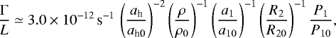
For large (100 km) asteroids with relatively small satellites, the situation is different. Radiative torques (cryptographically, ‘BYORP’) are considered weak because they scale as (Ćuk & Burns 2005):
 (1)
(1)
where Γ denotes the torque, L angular momentum, ah heliocentric semimajor axis, ρ density, a1 binary semimajor axis, P1 orbital period, and R2 secondary radius. The normalisation is given for ah0 = 1 au, ρ0 = 1750 kg m−3, a10 = 2 km, R20 = 0.15 km, P10 = 20 h, and synchronousrotation.
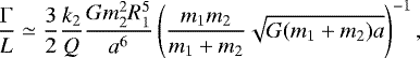
On the contrary, tides scale as (de Pater & Lissauer 2010):
 (2)
(2)
where k2 denotes the Love number, Q quality factor, R1 primary radius, and m1, m2 are the component masses. Tides are known to operate in planet–moon systems where dissipation occurs inside the planet. More precisely, they are measured for the Earth–Moon system, where Ṗ0 = 5.4 × 10⁻¹³ d d−1 (primary rotation period) and Ṗ1 = 1.1 × 10⁻¹¹ (secondary orbital period; equivalent to the orbital expansion of the Moon 0.038 m y−1). Sometimes, dissipation must occur in the moon to explain the observed orbits (e.g. Phobos; Rosenblatt 2011) or volcanism (Io; Peale et al. 1979; Morabito et al. 1979). There is no reason why 100 km asteroids should be different from other bodies, except for their material properties. Unfortunately, no such measurements exist for the moons of such large asteroids.
In this paper, we focus on the (216) Kleopatra moon system (Ostro et al. 2000; Descamps et al. 2011; Hirabayashi & Scheeres 2014; Shepard et al. 2018; Marchis et al. 2021; Brož et al. 2021). On October 10 1980, an occultation of Kleopatra itself was observed together with a serendipitous occultation event, which was later attributed to the outer moon of Kleopatra, and was designated S/2008 (216) 1, or I Alexhelios (Descamps et al. 2011). The event lasted only 0.9 s, but was observed by two independent observers separated by 0.61 km. Its sky position in the (u, v) plane coincided with the respective orbit of the outer (second) moon.
When we compared this observation with the revised ephemeris of Brož et al. (2021) – constrained by adaptive-optics (AO) datasets, hereafter denoted DESCAMPS, SPHERE2017, and SPHERE2018 – it turned out that the orbit orientation is very similar, but the predicted position is offset in the true longitude λ2 by approximately + 60° (see Fig. 1). The synthetic moon is farther away on its orbit. This certainly requires additional analysis, because it could be related to tides.
The occultation can hardly be associated with the inner (first) moon, because the distance between the sky-plane position and the orbit is more than 4.5σ at any given time, and the actual longitude λ1 is offset in the opposite direction by − 90° (alternatively, by as much as + 270°).
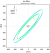 |
Fig. 1 Sky-plane projection of moons orbiting (216) Kleopatra, with the observed position of the occultation (black circle) from October 10, 1980, and the corresponding chord (dashed line) from Descamps et al. (2011). For comparison, both inner and outer moon orbits are plotted (green, blue; bodies 2, 3). The projected orbital velocity is indicated by an arrow. The ephemeris with constant osculating periods derived from adaptive-optics datasets (2008–2018) is offset by ~ 60° in the true longitude λ2 (black cross, orange line). This offset corresponds to a shorter orbital period P2 in the past. |
2 Observed tidal evolution
2.1 Increasing orbital period P2
Naïvely, we expected that a minor change of the osculating period P2 within the present uncertainty would be sufficient, but it was not. Indeed, the time-span of the AO datasets (2008–2018, or 3780 d) is comparable with the preceding occultation (1980–2008, 10220 d). Moreover, their phase coverage constrains both periods P1, P2.
To demonstrate this clearly, we computed simplified periodograms as follows. We used our previous converged model (Brož et al. 2021) to determine the true longitudes λ2 (unfolded) and orbital epochs Ei of all 2008–2018 observationswith respect to T0 = 2 454 728.761806. We then added one point corresponding to the 1980 occultation with the respective epoch Ei =λ2∕(2π) = 0.55. We assumed uncertainties of σE = 0.001, which corresponds to an astrometric uncertainty of about 10 mas. These data were compared with two simplified ephemerides – constant mean period1 (linear epoch):
 (3)
(3)
or linear period (quadratic epoch):
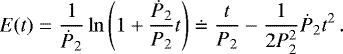 (4)
(4)
The difference between Ei, E(t), expressed as χ2, is plotted in Fig. 2. It is not possible to fit all epochs Ei with any of the constant periods. The structure of the periodograms is determined by the AO datasets, not by the occultation. On the other hand, a linearly variable period, with a suitable derivative Ṗ2 = (1.8 ± 0.1) × 10−8 d d−1, is satisfactory (and better by two orders of magnitude).
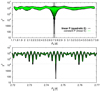 |
Fig. 2 Simplified periodograms for the second moon, obtained as a χ2 difference between the observed epochs Ei and computed epochs E(t) for constant mean periods P2 (green line), and linearly variable periods P2(t) = P2(0) + Ṗ2t (black line). The value Ṗ2 = 1.8 × 10⁻⁸ d d−1 corresponds to the offset of λ2 in Fig. 1. The grey box in the upper panel shows a range of the bottom panel. |
2.2 Monopole model including tides
Tidal dissipation in Kleopatra is a likely dynamical mechanism explaining the secular evolution of the orbital period P2. To determine the basic parameters of the tides, we used a time-lag model (Mignard 1979; Neron de Surgy & Laskar 1997). The additional acceleration (and torque) was implemented in the SWIFT integrator (Levison & Duncan 1994) as follows:
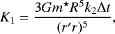
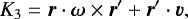
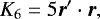
![Mathematical equation: \begin{equation*}\vec f_{\textrm{tides}} = K_1 \left[K_2\vec r\prime - K_3\vec r - K_4 (\vec r\times\vec\omega + \vec v) + K_5(K_6\vec r - K_7\vec r\prime)\right],\end{equation*}](/articles/aa/full_html/2022/01/aa42055-21/aa42055-21-eq5.png) (5)
(5)
 (6)
(6)
![Mathematical equation: \begin{equation*}K_2 = {5\over r\prime^2} \left[\vec r\prime\!\!\cdot\!\vec r\,(\vec r\cdot\vec\omega\times\vec r\prime\! + \vec r\prime\!\cdot\vec v)- {1\over 2r^2}\vec r\cdot\vec v (5(\vec r\prime\!\!\cdot\!\vec r)^2 - {r\prime}^2 r^2)\right],\end{equation*}](/articles/aa/full_html/2022/01/aa42055-21/aa42055-21-eq7.png) (7)
(7)
 (8)
(8)
 (9)
(9)
 (10)
(10)
 (11)
(11)
 (12)
(12)
 (13)
(13)
The classical notation assumes an Earth–Moon–test particle, but this can be any triple system and any combination of bodies denoted by indices (i, j≠i, k≠i). Ergo, m⋆ denotes the mass of the Moon, m′ the mass of the test particle, R the radius of the Earth, k2 the Love number of the Earth, Δt the time-lag, r the vector Earth–Moon (i.e. perturbing body), v the orbital velocity of the Moon, r′ the vector Earth–test particle (interacting body), ω the spin rate vector of the Earth, and Γ the torque acting on the spin of Earth. This general formula is used to compute cross-tides among all triples. In our case, non-negligible interactions are expected for Kleopatra–first moon–first moon, Kleopatra–second moon–second moon; where the tidal dissipation occurs in Kleopatra itself. Both moons have to be accounted for, because they contribute to the total torque (spin-down). A simple Euler integrator is then used to evolve spins, assuming principal-axis rotation. The time steps were 0.02 d (orbital) and 1 d (spin).
There are three relevant radii of Kleopatra: R = 59.6 km (volume-equivalent), 69.0 km (surface-equivalent), and 135 km (maximal). The volume equivalent is commonly used, but if tidal dissipation happens in surface layers, the surface equivalent should be preferred. In case of Kleopatra, we decided to use the maximal radius, because the strongest dissipation is expected at the ‘extremes’ of the elongated body. Other parameters are the Love number k2 = 0.305 (here, we used the same value as for the Earth), and the moment of inertia I = 1.72 × 1028 kg m2, as derived from the ADAM model (Marchis et al. 2021). We varied only the time-lag and obtained Δt =47 s, meaning that the offset in true longitude is Δλ2 = −60° with respect to the model without tides, or ~0° with respect to the observation (occultation). The evolution is shown in Fig. 3. It is very smooth because we included only the monopole for Kleopatra and we overplotted orbits computed separately, without perturbations.
For comparison, the inner (first) moon should tidally evolve with Ṗ1 = 5.0 × 10⁻⁸, which is inevitably larger than Ṗ2 = 1.8 × 10⁻⁸ due to the smaller distance. The accumulated change in the rotation phase of Kleopatra due to both moons over the entire time-span of 1980–2018 should then reach 1° (see Sect. 2.4).
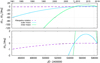 |
Fig. 3 Tidal evolution of Kleopatra spin (dashed magenta) and moon orbits (solid green, blue), computed as the difference in the true longitudes Δλ0, Δλ1, Δλ2 between dynamical models with and without tides. The value of the time-lag Δt = 47 s corresponds to Ṗ2 in Fig. 2. The epoch when mean periods coincide was arbitrarily shifted (↔) towards 2 456 500. Moreover, the mean periods were adjusted (↕) to fit observations in 2008 and 2018. |
2.3 Multipole model including tides
In order to have a complete dynamical model, we also implemented tides (Eqs. (5)–(13)) in Xitau2 (Brož 2017; Brož et al. 2021), which enabled us to fit all observations. Let us recall that the model already included multipoles up to the order ℓ = 10 and mutual moon perturbations, and that our previous best-fit model (Brož et al. 2021; without the 1980 occultation) had χ2 = 368 3.
We proceeded in several steps: (i) we unsuccessfully tried to re-converge periods P1, P2 (without tides), but the value of χ2 remained too high, at χ2 = 677, compared to the number of measurements (reported in Table 1); (ii) we successfully converged P1, P2 together with a non-zero time-lag Δt and obtained χ2 = 388; (iii) we verified there is no deeper local minimum in the surroundings (see Fig. 4); and (iv) we converged all remaining parameters, with the final χ2 = 360 (see Fig. 5). The respective parameters are presented in Table 1.
Although multipole perturbations (4 km in a2) or mutual perturbations (2 km) are orders of magnitude larger than tides (1 m yr−1 in ȧ2), the former are strictly conservative, or periodic, and the latter are dissipative, or non-periodic. Tides are crucial to explain the 1980 occultation.
Moreover, the tidal evolution may partially explain the systematic errors in our previous fitting of the SPHERE2017 dataset. When the osculating periods are constant and constrained by DESCAMPS and SPHERE2018, some offsets (of the order of 10 mas) are required for the intermediate dataset, especially for the first moon which is more affected by tides. A detailed comparison shows that the offsets may be decreased when tides are included (see Fig. 6). However, tidal evolution cannot explain all remaining systematic errors (cf. our discussion of astrometry in Brož et al. 2021).
2.4 Possibly increasing rotation period P0
As discussedin Sect. 2.2, if the moons are affected by tides, so must be the rotation of Kleopatra. If the period is evolving in time, then the value of P0 = 5.3852824(10) h reported by Marchis et al. (2021) corresponds to the middle of the 1977–2018 time-span. To estimate a realistic uncertainty of this ‘mean’ rotation period, we created 1000 bootstrapped samples of the light-curve data set (random selection of light curves and randomselection of points in those light curves) and used them as input for convex light-curve inversion. The data set of Marchis et al. (2021) was supplemented with other observations that are listed in Table A.1, and now consists of 198 light curves covering the interval 1977–2021. This led to the mean rotation period of:
 (14)
(14)
This improved uncertainty of the rotation period corresponds to uncertainty in Kleopatra’s rotation phase of 1.3° over the interval of 44 yr, which is of the same order as the expected 1° shift estimated in Sect. 2.2.
To check whether or not the predicted deceleration of the main body’s rotation is ‘visible’ in the data, we divided light curves into two sets: the first one covering the interval 1977–1994 and the second one 2002–2021. If the rotation period is changing, we should see some difference in the periods for these two data sets. Similarly, as with the full data set, we created 1000 bootstrapped samples and performed the light curve inversion independently for all of them to estimate parameter errors. For the interval 1977–1994, the rotation period was:
 (15)
(15)
and the corresponding phase shift 1.8°. For 2002–2021, the values were:
 (16)
(16)
and 1.0°. The uncertainty intervals are therefore larger (due to the shorter time span) than with the full data set and they overlap, that is, there is no indication that the rotation period is changing. Controversially, the mean period derived from 1977–2021 observations is slightly longer than periods for 1977–1994 and 2002–2021 subsets, while we would expect it to be somewhere in between the two values. This is partly caused by the correlation between the period and the pole direction (which is also optimised for each bootstrapped sample), but we think that the main reason is some small but systematic errors present in some of the light curves.
To test the sensitivity of our approach, we generated an equivalent set of synthetic observations using the non-convex ADAM shape model from Marchis et al. (2021), Hapke’s light-scattering model, and two values of Ṗ0, 3.2 × 10⁻¹² and 1.6 × 10⁻¹². We then treated the synthetic data set as real data and applied the same bootstrap approach to detect possible changes in rotation period. For Ṗ0 ≃ 3.2 × 10⁻¹², the effect of changing period was clearly visible as a systematic difference between periods for 1977–1994 and 2002–2021 data. In this way, we checked that the choice of using convex or non-convex models does not affect the results in a systematic way. However, when using Ṗ0 ≃ 1.6 × 10⁻¹² and adding 2% random noise to our synthetic light curves (which is a realistic estimate of observational uncertainties), the effect of changing period was no more detectable – both subsets of bootstrapped light curves had statistically the same rotation period.
We also tried to detect a possible evolution of Kleopatra’s rotation period by including Ṗ0 as a free parameter in the light curve inversion. In practice, we used the same approach as Kaasalainen et al. (2007) or Ďurech et al. (2018) when searching for the YORP effect that influences light curves in the same way – rotation period changes linearly over time (more precisely, angular velocity changes linearly over time but the difference is negligible). We used the same bootstrap sample as inthe case of fitting light curves with a constant-period model. The results are shown in Fig. 7, where P0 is plotted against Ṗ0. There is a strong anticorrelation between these two parameters – positive Ṗ0 (deceleration of the rotation) and shorter initial rotation (at the beginning of the observing time interval in 1977) has a similar outcome as negative Ṗ0 (acceleration of the rotation) and slower initial rotation. From bootstrap, Ṗ = (−0.5 ± 4.2) × 10−12, which means that the effect we are searching for, Ṗ0 = 1.9 × 10⁻¹², is consistent with the data but cannot be confirmed. Zero Ṗ0 is also compatible with the data. Due to correlation, the marginal uncertainty of P0 is 0.0000009 h, which is larger than when assuming Ṗ0 = 0.
Best-fit models with no tides (left) and including tides (middle), together with realistic uncertainties of the parameters (right).
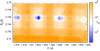 |
Fig. 4
|
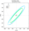 |
Fig. 5 Same as Fig. 1, but for our new multipole model including tides. The offset in true longitude λ2 is negligible (comparable to the uncertainty). |
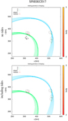 |
Fig. 6 Details of some SPHERE2017 astrometric observations and converged models with no tides (top) and including tides (bottom). The assumed uncertainties (10 mas) are indicated by black circles, and residuals are shown as red or orange lines. There is a noticeable improvement for the first moon. However, the second moon is still offset, possibly because of some remaining systematic error. The proper motion in the (u, v) plane is relatively slow because of the orbit orientation and the line of sight. |
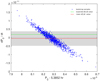 |
Fig. 7 Period P0 and its change Ṗ0 for 1000 bootstrap samples of the photometric data set. Each blue point represents one bootstrap run. The mean value − 0.5 × 10⁻¹² of Ṗ0 is marked with a red line, and the theoretical prediction 1.9 × 10⁻¹² of Kleopatra’s deceleration due to tides is marked with the green line. The grey strip marks the 1σ uncertainty interval for Ṗ. |
2.5 Discussion of the quality factor Q
Our modelling of tidal evolution indicates the time-lag around Δt = 42 s, with the assumed Love number of k2 ≐0.3. According to the approximate relation (Efroimsky & Lainey 2007):
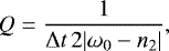 (17)
(17)
where Q denotes the quality factor, ω0 ≡ 2π∕P0 the spin rate, and n2 the mean motion, Q = 40, or Q∕k2 = 131. This Q value is relatively low (i.e. dissipation high), which seems reasonable for (216) Kleopatra – an irregular body close to critical rotation (Marchis et al. 2021). The value of k2 cannot realistically be orders-of-magnitude lower, because Q would be unrealistically low. For comparison, the Earth and Moon have Q = 280 ± 60 and 38 ± 4, respectively (Konopliv et al. 2013; Lainey 2016), but they correspond to low loading frequencies, ξ ≡ 2|ω − n|, and the expected dependence Q(ξ) is positive (Q ∝ ξ0.3 for ξ ≳ 10−2 rad d−1; Efroimsky & Lainey 2007). This is demonstrated in Fig. 8.
For uniform bodies, there is a relation between the Love number k2 and the material rigidity μ (Goldreich & Sari 2009; Eq. (24)):
 (18)
(18)
where S denotes the surface area; the approximation holds for bodies with substantial μ (or small k2). Because we know Q∕k2, we can obtain μQ = 2.7 × 10⁷ Pa. This is the same order of magnitude as the estimate for 1 km asteroids (Scheirich et al. 2015), but is three orders of magnitude smaller than the value μQ ≃ 1010 Pa derived for other 100 km asteroids (Marchis et al. 2008a,b). We can also try to express μ = 6.7 × 10⁵ Pa (from k2), but this is not independently constrained. It seems compatible with loose material, or at least regolith-covered bodies.
There is also a relation to the regolith thickness (Nimmo & Matsuyama 2019; Eq. (6)):
 (19)
(19)
where f = 0.6 is the assumed friction coefficient. This gives l = 13 m. For non-spherical bodies, there may be significant deviations. In particular, when we used the maximum radius R and only a part of the surface is at this distance, the regolith needed to explain all the dissipation is probably accordingly thicker.
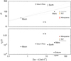 |
Fig. 8 Top: comparison of the quality factors Q for terrestrial bodies and Kleopatra, which experience different loading frequencies ξ ≡ 2|ω− n|. Data are from Lainey (2016). For Io and Kleopatra, Q was estimated from Q∕k2 and k2 ≐0.3. The value denoted ‘3:2’ was derived for Kleopatra when its moons are locked in the 3:2 resonance (see Sect. 2.6). Similarly, ‘massive’ is for the model with more massive moons (see Sect. 2.7). The dotted line is the expected dependence of Q(ξ) (normalised with respect to the Moon; Efroimsky & Lainey 2007). Bottom: comparison of the ratios k2 ∕Q and ξ, which are directly constrained by the respective tidal evolution. Kleopatra’s value is slightly above terrestrial bodies. |
2.6 Q for orbits in the 3:2 resonance
The orbits of the two moons appear to be very close to the 3:2 mean-motion resonance; the respective critical angle σ does not librate though, because orbits are so perturbed by the multipoles of Kleopatra and eccentricities are too small (Brož et al. 2021). Nevertheless, if they are locked, tides act on both moons at the same time and, inevitably, Ṗ2 = 1.5Ṗ1. According to our numerical experiments (using the machinery of Sect. 2.2), the value of Ṗ1 decreases and Ṗ2 increases compared to their nominal values. In order to obtain the same offset of Δλ2 = +60°, the required values are now Ṗ0 = 0.9 × 10⁻¹², Ṗ1 = 1.2 × 10⁻⁸, and Ṗ2 = 1.8 × 10⁻⁸. This corresponds to a time-lag of approximately Δt1 = 22 s.
Consequently, the dissipation factor as well as other derived quantities from Sect. 2.5 are revised as follows: Q = 76, Q∕k2 = 250, μQ = 5.0 × 10⁷ Pa, and l = 9 m. The assumption of the 3:2 resonance thus decreases the dissipation rate and puts Kleopatra somewhat closer to the theoretical dependence of Q(ξ) in Fig. 8.
 |
Fig. 9 Torque Γ over angular momentum L (in y−1 units) for the tidal (black), strong radiative (red), and weak radiative torques (orange). Relevant radial distances r are indicated (vertical dotted lines): the maximum radius R1 of the primary, Roche radius |
2.7 Q for more massive moons
In an alternative model, moons can be more massive (more dense than Kleopatra), with m2 = 4 × 10⁻¹⁶ MS and m3 = 9 × 10⁻¹⁶ MS (Brož et al. 2021), and the deformation potential is proportionally larger (Eq. (6)). Again, to obtain Δλ2 = +60°, Δt2 = 16 s is required, together with Ṗ0 = 3.6 × 10⁻¹², Ṗ1 = 3.1 × 10⁻⁸, and Ṗ2 = 1.8 × 10⁻⁸. The value of P0 is increased substantially, but still not enough to be confirmed (or excluded) by observations. Adjustments of other parameters are as follows: Q = 100, Q∕k2 = 330, μQ = 8.2 × 10⁷ Pa, and l = 13 m. This puts Kleopatra even closer to the theoretical dependence on Fig. 8 and indicates that mechanical properties of Kleopatra’s material may actually be similar to those of terrestrial bodies.
2.8 Discussion of the origin
Regarding the origin of the moons, it is interesting to estimate the timescale as the angular momentum over the tidal torque, L2 ∕Γ2 ≃ 1.3 × 10⁶ yr, because thiswould indicate the moons are very young. The dependence of both tidal and radiative torques, computed for the Kleopatra system according to Eqs. (1) and (2), is shown in Fig. 8. If the initial distance coincided with the last stable orbit (LSO), at about rlso= 280 km (or P ≃ 0.8 d) according to our numerical tests, and the final distance is comparable to half of the Hill sphere, rH = 33 100 km, the overall evolution would take over 2 × 10⁸ yr 4. In a broader perspective, this is comparable to the dynamical timescale of the rings of Saturn (Charnoz et al. 2009; although cf. Crida et al. 2019).
The moons are definitely younger than Kleopatra, because a large-scale collisional event would leave observable traces (an asteroid family). The moons may alternatively be related to small-scale craterings, which are much more frequent. Of the three following options, the latter appears the most plausible: (i) a cratering with a direct re-accretion of multi-kilometre moons; (ii) a collisional spin-up of Kleopatra over its critical frequency and mass shedding; (iii) low-speed ejection of material from the surface below the L1 critical point (see Fig. 6 in Marchis et al. 2021) and continuous accretion from ring. This suggested mechanism requires lower kinetic energy of collisions.
However, the long-term evolution could be complicated. If Kleopatra has been close to its rotation limit for a prolonged period of time, many moons have likely been created. This implies there are perhaps more moons within the Hill sphere, as suggested by some Keck images. The most likely distance seems to be about 1500 km, where Γ∕L is lowest and evolution is slowest. Such a hypothetical third moon would be close to the 3:1 resonance with the second moon and capture is inevitable. Subsequent evolution of eccentricity, which is increased by tides (Goldreich 1963; Correia et al. 2012), would lead to an instability of the moon system and an ejection of one or two moons beyond the Hill sphere. The timescale of evolution is determined by the inner moon. The instability may be delayed by the protective resonant mechanism, or alleviated if the moons have been rotating synchronously (1:1) and dissipating due to higher tidal modes (3:2, 2:1).
3 Conclusions
Astrometric and occultation observations of Kleopatra’s outer moon indicate a secular evolution of its orbital period Ṗ2 = (1.8 ± 0.1) × 10−8, which is the first such observation in a system of moons orbiting a large (100 km) asteroid. This should be linked to the secular evolution of the rotation period Ṗ0 = 1.9 × 10⁻¹² of (216) Kleopatra itself. The latter value is not excluded by current photometric observations, but their precision (about 1° in phase, or 3 miliseconds in period) is still not sufficient to exclude Ṗ0 = 0.
For future observers, we predict a secular evolution of the first moon Ṗ1 ≃ 5.0 × 10⁻⁸, which is inevitable when the second moon is driven by tides. If the observed value is found to be different, this could indicate, for example, stronger mutual interactions, different masses of the moons (m2, m3), or a greater proximity to the 3:2 mean-motion resonance. If the moons are inside the 3:2 resonance, the tides acting on the first moon also act on the second moon, and a lower dissipation in Kleopatra is sufficient to explain the offset in true longitude λ2. In more complex rheological models the time-lag Δt (or Q) also depends on loading frequencies, i.e. 2|ω − n|. However, in the Kleopatra triple system, the loading frequencies are perhaps too close (49.1, 51.4 rad d−1) to measure this dependence directly by means of accurate astrometry.
At the same time, adaptive-optics observations of fast-moving shadows (at higher phase angles) could perhaps be used to better constrain the rotation phase of Kleopatra and detect a possible difference between measured Ṗ0 and  inferred from tides (similarly as in the Earth–Moon system; cf. post-glacial rebound). Consequently, ground-based observations with the VLT/SPHERE instrument have the potential to constrain the ‘geophysical’ internal evolution of large asteroids.
There will be another opportunity to observe (216) Kleopatra and its moons in 2022–2024. According to our ephemeris, transits and eclipses of the moons will occur (e.g. Fig. 9). The intervals when orbital planes cross Kleopatra are as follows:
2022.34–2022.41 May 2.32 au
2022.80–2022.87 Oct.–Nov. 1.34 au
2023.93–2024.05 Dec.–Jan. 1.94 au
2024.51–2024.59 July 3.70 au.
Adaptive-optics and possibly also precise photometric observations could help to constrain the sizes and albedos of the moons. This is also true for stellar occultations (see Appendix B). Regarding hypothetical moons separated by 1500 km or more, whereradiative torques should be dominant, a deeper survey with the next-generation AO instruments like VLT/ERIS or Gemini/GPI2 would be useful.
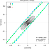 |
Fig. 10 Sky-plane projection of Kleopatra and moon orbits for the Besselian year 2022.80 (October), i.e. one of the epochs when eclipses and transits will be observable. The spacing between points corresponds to 0.02 d. Approximate sizes of the moons are 10 km, corresponding to 5 mas. |
Acknowledgements
We thank an anonymous referee for comments. This work has been supported by the Czech Science Foundation through grant 21-11058S (M. Brož, D. Vokrouhlický), 20-08218S (J. Ďurech, J. Hanuš), and by the Charles University Research program No. UNCE/SCI/023. This material is partially based upon work supported by the National Science Foundation under Grant No. 1743015. B.C. and P.V. were supported by CNRS/INSU/PNP. This work uses optical data from the Courbes de rotation d’astéroïdes et de comètes database (CdR, http://obswww.unige.ch/behrend/page_cou.html). The data presented herein were obtained partially at the W. M. Keck Observatory, which is operated as a scientific partnership among the California Institute of Technology, the University of California and the National Aeronautics and Space Administration. The Observatorywas made possible by the generous financial support of the W. M. Keck Foundation. The authors wish to recognize and acknowledge the very significant cultural role and reverence that the summit of Maunakea has always had within the indigenous Hawaiian community. We are most fortunate to have the opportunity to conduct observations from this mountain.
Appendix A List of new light curves
Observational circumstances of new light curves are provided in Table A.1.
New optical disk-integrated lightcurves of (216) Kleopatra used in this work.
Appendix B Predictions for stellar occultations 2022–2026
Predictions of the positions of Kleopatra’s moons for expected stellar occultations 2022–2026 are plotted in Fig. B.1.
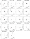 |
Fig. B.1 Predictions of the positions of Kleopatra’s moons in the (u, v) plane for the beginning time of expected stellar occultations in 2022–2026. Our ephemerides including tides (+) and without tides ( |

References
- Alton, K. B. 2009, Minor Planet Bull., 36, 69 [NASA ADS] [Google Scholar]
- Brož, M. 2017, ApJS, 230, 19 [Google Scholar]
- Brož, M., Marchis, F., Jorda, L., et al. 2021, A&A, 653, A56 [Google Scholar]
- Charnoz, S., Dones, L., Esposito, L. W., Estrada, P. R., & Hedman, M. M. 2009, Saturn After Cassini-Huygens, Origin and Evolution of Saturn’s Ring System, eds. M. K. Dougherty, L. W. Esposito, & S. M. Krimigis (Berlin: Springer), 537 [Google Scholar]
- Correia, A. C. M., Boué, G., & Laskar, J. 2012, ApJ, 744, L23 [NASA ADS] [CrossRef] [Google Scholar]
- Crida, A., Charnoz, S., Hsu, H.-W., & Dones, L. 2019, Nat. Astron., 3, 967 [NASA ADS] [CrossRef] [Google Scholar]
- Ćuk, M., & Burns, J. A. 2005, Icarus, 176, 418 [Google Scholar]
- de Pater, I., & Lissauer, J. J. 2010, Planetary Sciences (USA: NASA) [CrossRef] [Google Scholar]
- Descamps, P., Marchis, F., Berthier, J., et al. 2011, Icarus, 211, 1022 [NASA ADS] [CrossRef] [Google Scholar]
- Ďurech, J., Vokrouhlický, D., Pravec, P., et al. 2018, A&A, 609, A86 [NASA ADS] [CrossRef] [EDP Sciences] [Google Scholar]
- Efroimsky, M., & Lainey, V. 2007, J. Geophys. Res. Planets, 112, E12003 [NASA ADS] [CrossRef] [Google Scholar]
- Goldreich, P. 1963, MNRAS, 126, 257 [NASA ADS] [Google Scholar]
- Goldreich, P., & Sari, R. 2009, ApJ, 691, 54 [NASA ADS] [CrossRef] [Google Scholar]
- Hirabayashi, M., & Scheeres, D. J. 2014, ApJ, 780, 160 [Google Scholar]
- Kaasalainen, M., Ďurech, J., Warner, B. D., Krugly, Y. N., & Gaftonyuk, N. M. 2007, Nature, 446, 420 [NASA ADS] [CrossRef] [Google Scholar]
- Konopliv, A. S., Park, R. S., Yuan, D.-N., et al. 2013, J. Geophys. Res. Planets, 118, 1415 [NASA ADS] [CrossRef] [Google Scholar]
- Lainey, V. 2016, Celest. Mech. Dyn. Astron., 126, 145 [NASA ADS] [CrossRef] [Google Scholar]
- Levison, H. F., & Duncan, M. J. 1994, Icarus, 108, 18 [NASA ADS] [CrossRef] [Google Scholar]
- Marchis, F., Descamps, P., Baek, M., et al. 2008a, Icarus, 196, 97 [NASA ADS] [CrossRef] [Google Scholar]
- Marchis, F., Descamps, P., Berthier, J., et al. 2008b, Icarus, 195, 295 [NASA ADS] [CrossRef] [Google Scholar]
- Marchis, F., Jorda, L., Vernazza, P., et al. 2021, A&A, 653, A57 [NASA ADS] [CrossRef] [EDP Sciences] [Google Scholar]
- Mignard, F. 1979, Moon Planets, 20, 301 [Google Scholar]
- Morabito, L. A., Synnott, S. P., Kupferman, P. N., & Collins, S. A. 1979, Science, 204, 972 [NASA ADS] [CrossRef] [Google Scholar]
- Neron de Surgy, O., & Laskar, J. 1997, A&A, 318, 975 [NASA ADS] [Google Scholar]
- Nimmo, F., & Matsuyama, I. 2019, Icarus, 321, 715 [NASA ADS] [CrossRef] [Google Scholar]
- Ostro, S. J., Hudson, R. S., Nolan, M. C., et al. 2000, Science, 288, 836 [CrossRef] [Google Scholar]
- Pál, A., Szakáts, R., Kiss, C., et al. 2020, ApJS, 247, 26 [CrossRef] [Google Scholar]
- Peale, S. J., Cassen, P., & Reynolds, R. T. 1979, Science, 203, 892 [Google Scholar]
- Rosenblatt, P. 2011, A&ARv, 19, 44 [CrossRef] [Google Scholar]
- Scheirich, P., Pravec, P., Jacobson, S. A., et al. 2015, Icarus, 245, 56 [CrossRef] [Google Scholar]
- Scheirich, P., Pravec, P., Kušnirák, P., et al. 2021, Icarus, 360, 114321 [CrossRef] [Google Scholar]
- Shepard, M. K., Timerson, B., Scheeres, D. J., et al. 2018, Icarus, 311, 197 [NASA ADS] [CrossRef] [Google Scholar]
These mean Keplerian periods are different from osculating periods reported in Brož et al. (2021) by a factor of approximately 1.02246.
More specifically, the individual contributions were  (absolute astrometry),
  (relative astrometry),
  (adaptive-optics), and the joint metric was given as
 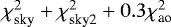 .
.
Assuming the BYORP were not interrupted by periods of non-synchronous rotation of the moon.
All Tables
Best-fit models with no tides (left) and including tides (middle), together with realistic uncertainties of the parameters (right).
All Figures
|
Fig. 1 Sky-plane projection of moons orbiting (216) Kleopatra, with the observed position of the occultation (black circle) from October 10, 1980, and the corresponding chord (dashed line) from Descamps et al. (2011). For comparison, both inner and outer moon orbits are plotted (green, blue; bodies 2, 3). The projected orbital velocity is indicated by an arrow. The ephemeris with constant osculating periods derived from adaptive-optics datasets (2008–2018) is offset by ~ 60° in the true longitude λ2 (black cross, orange line). This offset corresponds to a shorter orbital period P2 in the past. |
| In the text | |
|
Fig. 2 Simplified periodograms for the second moon, obtained as a χ2 difference between the observed epochs Ei and computed epochs E(t) for constant mean periods P2 (green line), and linearly variable periods P2(t) = P2(0) + Ṗ2t (black line). The value Ṗ2 = 1.8 × 10⁻⁸ d d−1 corresponds to the offset of λ2 in Fig. 1. The grey box in the upper panel shows a range of the bottom panel. |
| In the text | |
|
Fig. 3 Tidal evolution of Kleopatra spin (dashed magenta) and moon orbits (solid green, blue), computed as the difference in the true longitudes Δλ0, Δλ1, Δλ2 between dynamical models with and without tides. The value of the time-lag Δt = 47 s corresponds to Ṗ2 in Fig. 2. The epoch when mean periods coincide was arbitrarily shifted (↔) towards 2 456 500. Moreover, the mean periods were adjusted (↕) to fit observations in 2008 and 2018. |
| In the text | |
|
Fig. 4
|
| In the text | |
|
Fig. 5 Same as Fig. 1, but for our new multipole model including tides. The offset in true longitude λ2 is negligible (comparable to the uncertainty). |
| In the text | |
|
Fig. 6 Details of some SPHERE2017 astrometric observations and converged models with no tides (top) and including tides (bottom). The assumed uncertainties (10 mas) are indicated by black circles, and residuals are shown as red or orange lines. There is a noticeable improvement for the first moon. However, the second moon is still offset, possibly because of some remaining systematic error. The proper motion in the (u, v) plane is relatively slow because of the orbit orientation and the line of sight. |
| In the text | |
|
Fig. 7 Period P0 and its change Ṗ0 for 1000 bootstrap samples of the photometric data set. Each blue point represents one bootstrap run. The mean value − 0.5 × 10⁻¹² of Ṗ0 is marked with a red line, and the theoretical prediction 1.9 × 10⁻¹² of Kleopatra’s deceleration due to tides is marked with the green line. The grey strip marks the 1σ uncertainty interval for Ṗ. |
| In the text | |
|
Fig. 8 Top: comparison of the quality factors Q for terrestrial bodies and Kleopatra, which experience different loading frequencies ξ ≡ 2|ω− n|. Data are from Lainey (2016). For Io and Kleopatra, Q was estimated from Q∕k2 and k2 ≐0.3. The value denoted ‘3:2’ was derived for Kleopatra when its moons are locked in the 3:2 resonance (see Sect. 2.6). Similarly, ‘massive’ is for the model with more massive moons (see Sect. 2.7). The dotted line is the expected dependence of Q(ξ) (normalised with respect to the Moon; Efroimsky & Lainey 2007). Bottom: comparison of the ratios k2 ∕Q and ξ, which are directly constrained by the respective tidal evolution. Kleopatra’s value is slightly above terrestrial bodies. |
| In the text | |
|
Fig. 9 Torque Γ over angular momentum L (in y−1 units) for the tidal (black), strong radiative (red), and weak radiative torques (orange). Relevant radial distances r are indicated (vertical dotted lines): the maximum radius R1 of the primary, Roche radius |
| In the text | |
|
Fig. 10 Sky-plane projection of Kleopatra and moon orbits for the Besselian year 2022.80 (October), i.e. one of the epochs when eclipses and transits will be observable. The spacing between points corresponds to 0.02 d. Approximate sizes of the moons are 10 km, corresponding to 5 mas. |
| In the text | |
|
Fig. B.1 Predictions of the positions of Kleopatra’s moons in the (u, v) plane for the beginning time of expected stellar occultations in 2022–2026. Our ephemerides including tides (+) and without tides ( |
| In the text | |
Current usage metrics show cumulative count of Article Views (full-text article views including HTML views, PDF and ePub downloads, according to the available data) and Abstracts Views on Vision4Press platform.
Data correspond to usage on the plateform after 2015. The current usage metrics is available 48-96 hours after online publication and is updated daily on week days.
Initial download of the metrics may take a while.