| Issue |
A&A
Volume 677, September 2023
|
|
|---|---|---|
| Article Number | A189 | |
| Number of page(s) | 19 | |
| Section | Planets and planetary systems | |
| DOI | https://doi.org/10.1051/0004-6361/202346386 | |
| Published online | 27 September 2023 | |
An advanced multipole model of the (130) Elektra quadruple system
1
Charles University, Faculty of Mathematics and Physics, Astronomical Institute,
V Holešovičkách 2,
18000
Prague, Czech Republic
e-mail: This email address is being protected from spambots. You need JavaScript enabled to view it.
2
Aix-Marseille Univ., CNRS, LAM, Laboratoire d’Astrophysique de Marseille,
13388
Marseille Cedex 13, France
3
Astronomical Institute of the Czech Academy of Sciences,
Fričova 298,
Ondřejov
25165, Czech Republic
Received:
11
March
2023
Accepted:
18
July
2023
Abstract
Context. The Ch-type asteroid (130) Elektra is orbited by three moons, making it the first quadruple system in the main asteroid belt.
Aims. We aim to characterise the irregular shape of Elektra and construct a complete orbital model of its unique moon system.
Methods. We applied the All-Data Asteroid Modelling (ADAM) algorithm to 60 light curves of Elektra, including our new measurements, 46 adaptive-optics (AO) images obtained by the VLT/SPHERE and Keck/Nirc2 instruments, and two stellar occultation profiles. For the orbital model, we used an advanced N-body integrator, which includes a multipole expansion of the central body (with terms up to the order ℓ = 6), mutual perturbations, internal tides, and the external tide of the Sun acting on the orbits. We fitted the astrometry measured with respect to the central body and also relatively, with respect to the moons themselves.
Results. We obtained a revised shape model of Elektra with the volume-equivalent diameter (201 ± 2) km. Of two possible pole solutions, (λ,β) = (189; −88) deg is preferred, because the other one leads to an incorrect orbital evolution of the moons. We also identified the true orbital period of the third moon S/2014 (130) 2 as P2 = (1.642112 ± 0.000400) days, which is in between the other periods, P1 ≃ 1.212days, P3 = 5.300 days, of S/2014 (130) 1 and S/2003 (130) 1, respectively. The resulting mass of Elektra, (6.606-0.013+0.007) ×1018 kg, is precisely constrained by all three orbits. Its bulk density is then (1.536 ± 0.038) g cm−3. The expansion with the assumption of homogeneous interior leads to the oblateness J2 = −C20 ≃ 0.16. However, the best-fit precession rates indicate a slightly higher value, ≃0.18. The number of nodal precession cycles over the observation time span 2014–2019 is 14, 7, and 0.5 for the inner, middle, and outer orbits.
Conclusions. Future astrometric or interferometric observations of Elektra’s moons should constrain these precession rates even more precisely, allowing the identification of possible inhomogeneities in primitive asteroids.
Key words: minor planets / asteroids: individual: (130) Elektra / planets and satellites: fundamental parameters / astrometry / celestial mechanics / methods: numerical
© The Authors 2023
 Open Access article, published by EDP Sciences, under the terms of the Creative Commons Attribution License (https://creativecommons.org/licenses/by/4.0), which permits unrestricted use, distribution, and reproduction in any medium, provided the original work is properly cited.
This article is published in open access under the Subscribe to Open model. This email address is being protected from spambots. You need JavaScript enabled to view it. to support open access publication.
1 Introduction
The asteroid (130) Elektra belongs to the primitive Ch spectral type objects (Rivkin et al. 2015). The visible and near-infrared spectral data for Ch- and Cgh-type asteroids most closely resemble those obtained for the unheated CM chondrite meteorites, and these asteroids therefore most likely represent their parent bodies (Vilas & Gaffey 1989; Vernazza et al. 2016). The only minor spectral variations among the largest Ch/Cgh bodies and the members of the associated collisional families are likely due to differences in the average grain size of the regolith particles. Therefore, CM parent bodies had homogeneous internal structures and did not experience significant (>300 °C) heating due to thermal evolution (Vernazza et al. 2016). Nevertheless, Elektra is not intact, because it experienced a collision, which is commonly the origin of small satellites (Durda et al. 2004; Benavidez et al. 2012).
Elektra is orbited by three satellites (also referred to as moons): S/2003 (130) 1 (Marchis et al. 2008), S/2014 (130) 1 (Yang et al. 2016), and S/2014 (130) 2 (Berdeu et al. 2022). The diameters of the moons as derived from their photometry are of the order of 6, 2, and 1.6 km. For the third moon, a short-periodic orbit was found, with a period of only 0.67 days (Berdeu et al. 2022).
Previous shape modelling of Elektra (Hanuš et al. 2017; Vernazza et al. 2021) indicates that the ecliptic latitude β is close to −88° or −89°. Hence, the ecliptic longitude λ remains poorly constrained, because even distant values of λ represent similar directions in space.
In this work, we revise the shape model together with the orbits of the moons. Most importantly, this helps us to resolve the ambiguity of poles, because the non-spherical shape of the central body induces a precession of the pericentres ω and nodes Ω, which is constrained by the astrometry of the moons. We also use additional photometric data, as described in Sect. 2.
From now on, bodies are denoted as follows: 0 – (130) Elektra, 1 – S/2014 (130) 1, 2 – S/2014 (130) 2, 3 – S/2003 (130) 1. As explained in Sect. 4, this order corresponds to the respective orbits: 1 – inner, 2 – middle, and 3 – outer. All physical and orbital quantities are numbered accordingly.
2 Data
2.1 Light curves, AO images, and stellar occultations of Elektra
For the shape reconstruction of Elektra, we prepared a data set consisting of 60 light curves, 46 AO images, and two stellar occultations. Most of the light curves (55 out of 60) were taken from the Database of Asteroid Models from Inversion Techniques (DAMIT1 ; Ďurech et al. 2010), which contains light curves and other input parameters in addition to shape models. The observational data covered the time span from 1980 to 2016. In March 2022, we expanded the set by measuring five new light curves (Table 1) using the BlueEye600 robotic observatory (Ďurech et al. 2018) located in Ondřejov. These light curves were obtained exclusively for this study and are now available in DAMIT together with the new shape and spin state solution. Moreover, we also uploaded them to the ACLDEF2 database. All of the light curves used in this study, including the new measurements, can be found in Appendix D.
The set of AO images consists of two subsets. The first one from Hanuš et al. (2017) consists of 14 images captured by the Keck/Nirc2 instrument during the years 2002-2012 and two high-resolution infrared images were taken by the AO system VLT/SPHERE in 2014. The InfraRed Differential Imager and Spectrograph (IRDIS; Dohlen et al. 2008) and the Integral Field Spectrograph (IFS; Claudi et al. 2008) were used simultaneously to cover a more extended spectral range. The second subset of 30 images is taken from Vernazza et al. (2021). It was obtained by the Zurich IMaging POLarimeter (ZIMPOL; Schmid et al. 2018) during the summer of 2019. The two stellar occultations were taken from the Asteroidal Occultation Observers in Europe3 database. The first event occurred on 21 April 2018 and was observed by 48 observers in total. After excluding 4 far misses and 6 chords with incorrect time indications, we were left with 38 usable chords. The second event occurred on 21 February 2021 and was observed by 17 observers. However, eight of the chords were non-detections. Although such chords are generally useful as ’strict’ bounds for the asteroid’s shape, we did not use them because the shape is already well constrained. Both occultation events are shown in Fig. 1.
Summary of optical disk-integrated light curves of (130) Elektra obtained in this work by the BlueEye600 robotic observatory.
2.2 Astrometric measurements of the moons
For the process of fitting the orbital parameters of the moons, it is crucial to have a sufficient set of positions, usually related to the central body or its photocentre. These positions were measured on the AO images of Elektra – with various methods – whenever some of its moons were visible.
The first data set was taken from Berdeu et al. (2022), where the process of reduction, halo removal, and astrometry is explained in detail. Their data set is based on individual AO images of Elektra from December 2014 and consists of 120 positions of S/2014 (130) 1, 120 positions of S/2014 (130) 2, and 150 positions of S/2003 (130) 1. However, it is important to note that the individual positions are not mutually independent. Indeed, they correspond to a linear fit (in time) of 40 or 50 unique measurements. The second data set is based on 30 AO images from Vernazza et al. (2021). The images were reduced using the eclipse data reduction package (Devillard 1997). After reduction, the images were separately processed to remove the bright halo surrounding the asteroid, which was a necessary step to improve the detectability of the moons. To obtain the astrometric positions of the satellites, we used a specialised algorithm (Hanuš et al. 2013) that extracted the primary’s contour and determined its photocentre. By fitting a Moffat-Gauss source profile to the moons and measuring from the photocentre, we obtained the 20, 20, and 12 new positions of the respective moons. Moreover, we computed the astrometric positions of the moons with respect to the other moons, which is handy to avoid any systematic related to the photocentre of the central body, or possibly centre-of-mass corrections.
The new positions are listed in Appendix B. Additionally, all astrometric data are available for download from the Xitau4 webpage.
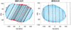 |
Fig. 1 Comparison of Elektra’s shape model to chords from occultation events. The red triangles represent the timing uncertainties at the ends of each chord and the dashed lines are non-detection chords. |
3 Shape reconstruction
3.1 All-Data Asteroid Modelling algorithm
The All-Data Asteroid Modelling (ADAM) algorithm (Viikinkoski et al. 2015) is a versatile inversion technique for the shape reconstruction of asteroids from various data types (AO images, light curves, occultations, radar, etc.). ADAM minimises the objective function, which is a measure of the difference between the Fourier-transformed image and the projected shape:
 (1)
(1)
where ℱDi(uij, υij) is the Fourier transform of the data image Di and ℱMi(uij,υij) is the Fourier transform of the projected shape Mi, corresponding to the ith image and evaluated at the jth frequency point (uij, υij). The scale si and offset ( ,
,  ) are free parameters resolved during the optimisation. The additional term
  is the standard square norm of the light-curve fit, while the term
  is the model fit to stellar occultation chords. The implementation of the latter term in ADAM is described in Hanuš et al. (2017). The first three terms are multiplied by their corresponding weights wAO , wLC, and wOC and the last term is a sum of regularisation functions γi multiplied by the weights wi (Viikinkoski et al. 2015; Hanuš et al. 2017).
The data weights have an impact on the initial convergence of χ2 and subjectively depend on the dataset; they are chosen to balance the individual χ2 values and enable good convergence. Regularisation weights then help guide the convergence during the process.
Two shape representations are supported: octantoids and subdivisions. Octantoids are a global parametrisation, whereas subdivisions offer more local control. In this work, we used the octantoid shape representation. For a more detailed explanation, see Viikinkoski et al. (2015).
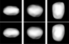 |
Fig. 2 Best-fit shape model (top) and the alternative shape model (bottom) from three different viewing geometries. The first two are equator-on views rotated by 90° and the third one is a pole-on view. The model is lit up artificially to highlight its finer surface details. |
3.2 Best-fit and alternative shape models
We took a two-step approach. First, we aimed to get just a coarse shape model. Second, the shape resulting from the first optimisation was used as an initial model, and we then doubled the number of facets and the spherical harmonics degree in order to capture surface details. The initial conditions for the convergence, which are needed for the period and the pole, were taken from Vernazza et al. (2021).
Figure 2 and Table 2 present the best-fit and alternative shape models and their parameters. The best-fit model is a revised version of the shape model published in Vernazza et al. (2021), which is based on a larger dataset. Its pole coordinates were allowed to converge along with the shape to best fit the data. The alternative model is a shape model that converged with the pole fixed according to the coordinates inferred from our orbital model (Sect. 4).
The χ2 map in Fig. 3 shows why the pole solution from ADAM remains unconstrained. Due to the close absolute distance of coordinates, there are many viable models. The best-fit model, denoted by a black tile, is in the upper left area of the map, while the alternative model is in a different local minimum in the bottom right area of the map. We propose that this alternative local minimum is where the true orbital pole lies. In Sect. 4, we even present a counterexample model based on the shape pole solution to support this.
We plotted a distribution of volume values from the dataset of models obtained from the χ2 mapping (Fig. 4). By looking at the 16%, 50%, and 84% percentiles of the distribution we determined the uncertainties of Deq in Table 2.
The comparison of these two models with several AO images from the 2019 data set is given in Fig. 5. In the comparison and Fig. 2, we see that the overall shape of the alternative model is more rounded, with fewer surface features in some areas. However, this is in the range of expected differences dependent on regularisations. Both models are statistically and visually almost identical.
In the last two columns of Fig. 5, we see that the local topography present in the two AO images is not captured by either of the models. We tried using the subdivision shape representation and locally forcing those features, but it seems that they are not supported by the rest of the dataset, and forcing them just makes the overall fit worse.
For both models, we used the following weights: wLC = 1·5, WAO = 0.85, wOC = 0.019, and standard values for the regularisation weights. In Appendix D, we compare the best-fit model to all the observed light curves.
Parameters of the best-fit (first line) and alternative (second line) models.
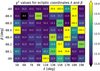 |
Fig. 3 χ2 map for pole coordinates λ and β, where each value of χ2 is represented by a colour from the colour bar. The black tiles indicate values below the range of the colour bar, while the yellow tiles indicate values above the range of the colour bar. |
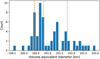 |
Fig. 4 Distribution of Deq values based on shape models with χ2 values below 12. The 16%, 50%, and 84% percentiles of the distribution are shown with orange lines. |
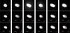 |
Fig. 5 AO images of Elektra (top), the best-fit shape model (middle), and the alternative shape model (bottom), all shown from the same viewing angle. The rotation axis is indicated by the red arrow. |
3.3 Multipole coefficients
Our orbital model has to be evolved over approximately 1000 days. On such a timescale, approximating the central body as a point mass is insufficient. Therefore, we computed a multipole expansion of the gravitational field up to the order of ℓ = 10. The expansion is based on the Delaunay triangulation of the ADAM shape model made using the TetGen program (Si 2006). The respective definitions of the multipole coefficients are as follows:
 (2)
(2)
 (3)
(3)
 (4)
(4)
where r, θ, ϕ are the body-frozen spherical coordinates, M the mass of the body, R the reference radius of the gravitational model, Pℓ, Pℓm the Legendre and associated Legendre polynomials, and Cℓm, Sℓm are the respective coefficients.
Table 3 lists the results of Eqs. (2)–(4) evaluated for our best-fit shape model with homogeneous density. We found that an expansion up to the order ℓ = 2 is sufficient to account for the precession of orbits and the higher orders (up to ℓ = 6) were used to confirm that their contribution is in fact negligible.
Most notable is the oblateness coefficient J2 = −C20 ≈ 0.159. This is a relatively high value; only a few 100 km asteroids have a similar c/a axial ratio to that of (l30) Elektra (Vernazza et al. 2021); for example (7) Iris, (16) Psyche, (22) Kalliope, and (45) Eugenia. The value inferred from shape will be compared to the dynamical oblateness in Sect. 4.6.
The alternative shape model has an almost equivalent J2 ≃ 0.162. This corresponds to an uncertainty of only 0.003. We verified that the discretisation error of J2 arising from the finite number of tetrahedrons is less than 0.001.
4 Orbital model
4.1 The dynamics included in the model
We use the N-body model called Xitau5 based on the Bulirsch-Stoer integrator from Levison & Duncan (1994) that was substantially modified (Brož 2017; Brož et al. 2021, 2022a) to include the multipole expansion (up to the order ℓ = 10), the tidal evolution, the external tides, and in particular, the fitting ’machinery’. To compare the model with the observations, we use the following unreduced metric6:
 (5)
(5)
![Mathematical equation: $\chi _{{\rm{sky}}}^2 = \sum\limits_{j = 1}^{{N_{{\rm{bod}}}}} {\sum\limits_{i = 1}^{{N_{{\rm{sky}}}}} {\left[ {{{{{\left( {{\rm{\Delta }}{u_{ji}}} \right)}^2}} \over {\sigma _{{\rm{sky}}\,{\rm{major}}\,ji}^2}} + {{{{\left( {{\rm{\Delta }}{\upsilon _{ji}}} \right)}^2}} \over {\sigma _{{\rm{sky}}\,{\rm{minor}}\,ji}^2}}} \right]} ,} $](/articles/aa/full_html/2023/09/aa46386-23/aa46386-23-eq11.png) (6)
(6)
![Mathematical equation: $\chi _{{\rm{sky2}}}^2 = \sum\limits_{i = 1}^{{N_{{\rm{sky2}}}}} {\left[ {{{{{\left( {{\rm{\Delta }}{u_i}} \right)}^2}} \over {\sigma _{{\rm{sky}}\,{\rm{major}}\,i}^2}} + {{{{\left( {{\rm{\Delta }}{\upsilon _i}} \right)}^2}} \over {\sigma _{{\rm{sky}}\,{\rm{minor}}\,i}^2}}} \right]} ,$](/articles/aa/full_html/2023/09/aa46386-23/aa46386-23-eq12.png) (7)
(7)
 (8)
(8)
where the index i corresponds to the observational data, j to individual bodies, k to angular steps of silhouette data, ′ to synthetic data interpolated to the times of observations, u, υ are the sky-plane coordinates, and σ the observational uncertainties along the two axes (denoted ‘major’ and ‘minor’ for ellipsoidal uncertainties).
The ‘goodness-of-fit’ terms  and
and  correspond to the absolute astrometry (i.e. with respect to body 0) and the relative astrometry (e.g. body 2 with respect to body 1). Optionally, we also include the regularisation term
  derived from silhouettes (as explained in Brož et al. 2021), which prevents pole orientations incompatible with the shape. This term is multiplied by the weight wao, which has no relation to the weight term wao from Eq. (1).
Using both  and
and  is useful because they are not exactly the same measurements. Computing the relative positions removes any systematics related to the photocentre and provides more precise (relative) information. We note that this rapidly increases the overall number of measurements, as each AO image where two or three moons are visible at the same time is counted again for each relative measurement taken.
In the following, we present two orbital models of increasing complexity. In both of them, we account for the external tide exerted by the Sun. The necessary ephemerides were obtained from the Jet Propulsion Laboratory (JPL; Park et al. 2021).
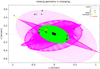 |
Fig. 6 Keplerian model of orbits 1 and 3 with χ2 = 2195 over the time-span of 1707 days. The orbits are plotted in the (u; υ) coordinates (green and pink lines, respectively), together with observed positions (black crosses), and residuals (red and yellow lines, respectively). Elektra’s shape for one of the epochs is over-plotted in black. |
Multipole coefficients (up to ℓ = 6) of Elektra’s gravitational field derived from the ADAM shape, assuming homogeneous density.
4.2 Keplerian model
Initially, by manual fitting and then by converging with the simplex algorithm (Nelder & Mead 1965), we constructed a simplified Keplerian model for the already well-known moons: S/2014 (130) and S/2003 (130), that is, a model of orbits 1 and 3. The masses of the moons were neglected and the central body was taken as a point of mass. These preliminary orbits are shown in Fig. 6.
In the case of the Elektra system, a Keplerian model is accurate enough for a time span of about a month, as can be seen in Berdeu et al. (2022), but is insufficient for the time span of 1707 days. The resulting value of χ2 = 2195 is too high compared to the number of measurements (i.e. 430). The residuals in
Fig. 6 exhibit large systematic uncertainties. In the top left part in particular, the synthetic orbit is far from that suggested by observations. This is due to the missing nodal precession, which must be present given the non-negligible oblateness (J2 = −C20) of the central body.
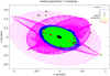 |
Fig. 7 Quadrupole model of the orbits 1, 2, and 3 with χ2 = 1084 over the time-span of 1707 days. The orbits are plotted in the (u; υ) coordinates (green, blue and pink lines, respectively), together with observed positions (black crosses) and residuals (red, orange and yellow lines, respectively). Elektra’s shape for one of the epochs is overplotted in black. |
4.3 Best-fit quadrupole model
We present a quadrupole model of the full system in Figs. 7 and 8. In this more complex model, the masses of the moons are taken into account and the gravitational field of the central body was expanded up to the order ℓ = 2 (according to Table 3), assuming homogeneous density. When evaluated with the full metric (Eq. (5)) with the weight wao = 0.3, the model is a best-fit one with χ2 = 1084.
This model is the result of a long series of models, which were being improved with every iteration. It was much more efficient to only use up to ℓ = 2, which is sufficient for a satisfying model.
We list the parameters of this best-fit model in Tables 4 and 5. They are given as osculating for the epoch T0 = 2457021.567880 (TDB), but these elements are not constant. Due to the oblateness of Elektra and its massive moons, the orbital elements oscillate over time, as can be seen in Figs. 9–11. The peak-to-peak amplitudes of some of these elements are substantial, and so it is not surprising that the Keplerian model is insufficient. From the circulation of the arguments of pericentre, we determined the apsidal precession of the moons:  ,
,  , and
, and  .
.
The uniqueness of our solution lies in the precession cycles of Ω and ϖ (Figs. 9–11). The two innermost orbits have many cycles; that is, about 14 cycles of Ω1 and ϖ1 and about 7 cycles of Ω2 and ϖ2. A correct orbital solution could be one with two and one cycle less, respectively. Thankfully, we also have the outer moon and its orbit with only a half cycle of Ω3 and ϖ3, which cannot be made one cycle more or less without being a completely different and unviable solution. Therefore, even the number of precession cycles of the two innermost moons is well constrained because the central body is the same.
Having the precise mass of Elektra,  , we can combine it with the volume of the shape model, (4.3 + 0.1) × 106 km3, and obtain the precise bulk density,
  Since we use multipole expansion, our orbital model sensitively depends on the orientation of the central body. Even a small change in the coordinates of the pole can completely change the satellite’s orbits. Indeed, we obtained more precise pole coordinates, λpole = (188.3 + 2.6) deg and βpole = (−88.2 + 0.2) deg, from our orbital model than from the shape model alone. Consequently, we derived an alternative shape model, as discussed in Sect. 3.
Notes, m are the masses of the individual bodies and a are the semi-major axes. The same notation as in Table 4 is used.
To demonstrate that these more precise pole coordinates are indeed preferable, we present a counterexample model in Table 4. This model is based on a rotational pole given by the ADAM algorithm in Sect. 3 and has a much higher χ2 value, making it unviable.
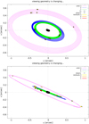 |
Fig. 8 Same as Fig. 7, but plotted separately for each data set: Berdeu et al. (2022, top) and Vernazza et al. (2021, bottom). |
Parameters of the best-fit model, given with uncertainties.
Dependent parameters of the best-fit model, given with uncertainties.
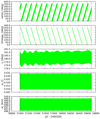 |
Fig. 9 Evolution of the osculating elements of the inner moon S/2014 1 plotted over the time span of 1707 days. Shown is the semimajor axis a1, eccentricity e1, inclination i1, the longitude of the ascending node Ω1, and the longitude of the periapsis ϖ1. |
4.4 M CMC analysis
The Markov chain Monte Carlo (MCMC; Robert & Casella 2011; Tierney 1994) is a method for randomly sampling probability distributions. To sample the distribution functions of the parameters of our orbital model we used the Python package emcee (Foreman-Mackey et al. 2013), which is an implementation of the MCMC.
We let all parameters of the model be free, including the rotational pole of Elektra, the total mass of the system, the mass ratios of the moons q1, q2, and q3, and 18 orbital parameters, six for each orbit of the three moons. To initialise the chains, we started with the parameters of the best-fit model and set some a priori limits to keep the walkers around the local minimum of our preferred solution. The limits were an order of magnitude higher and lower for q1, q2 and q3 to test if they are constrained, and a range of a few hours for the orbital periods. For other variables, the limits are relevant only in the case of Ω1 and λ1, because some part of their distribution lies beyond their upper limits, as can be seen in Fig. A.1. However, this should not notably affect the results.
We ran the MCMC with 48 walkers (i.e. two times 24; the number of free parameters) for 4000 iterations. However, as our limits on orbital periods were not narrow enough, about 15 walkers ended up migrating into neighbouring local minima, and so without the loss of generality, we removed them. We set the burn-in phase as 2000 iterations; after that, almost all parameters were in a steady state (Fig. A.2), except for q1, q2, log e2, and Ω2 (and therefore ϖ2 and λ2), which still have some overall upward or downward trends. Regardless, this again should not notably affect the results.
From the MCMC, we obtained the uncertainties on the parameters. These are given in Table 4 at 1σ, also known as the 16% and 84% percentiles. In particular, we have a very precise determination of the total mass, because it was constrained by all three orbits.
The complete corner plot is shown in Fig. A.l. Some of the parameters are correlated with each other. First, we have a strong positive triple correlation in each set of Ωi, ϖi, and λi, where i = 1, 2, 3. This is not surprising given the definitions of these parameters. The third triplet also has a positive correlation with log e3. This could be explained by the specific observation geometry during the respective epochs. The log e3 also has a negative correlation with i3, which could also be due to the different observation geometries. Lastly, the first triplet has a positive correlation with the mass ratio q3.
4.5 The third moon, S/2014 (130) 2
The Kepler solution presented by Berdeu et al. (2022) is a short-period (0.67 day) orbit of the third moon S/2014 (130) 2. However, it appears to ‘cross’ the orbit of the inner moon S/2014 (130) 1. Here, we present a 4-body model, which includes mutual interactions, multipoles (ℓ = 2), and external tides. We surveyed all possible periods and tested both inner and outer orbits. In particular, we were interested in a co-orbital solution because the astrometric positions of S/2014 (130) 2 are always close to the orbit of S/2014 (130) 1.
The periodogram for the third moon is presented in Fig. 12. Its orbit is unstable below 0.58 day; 0.67 day is only one local minimum, but undeniably not the deepest. The co-orbital solutions have periods between 1.19 and 1.20 days, but none of them are deep enough, unfortunately. A regular series of minima is seen for longer periods, with 1.64 days being the deepest minimum.
This minimum is our preferred solution for S/2014 (130) 2. It is a stable orbit, close to the mean-motion resonance with S/2014 (130) 1. The ratio of periods 1.35 is not exactly 4/3, because of the respective critical angle:
 (9)
(9)
or alternatively:
 (10)
(10)
includes a non-negligible precession contribution. Nevertheless, neither of these angles librates; a necessary period for an exact resonance is slightly shorter, P2 = 1.608 days. Nonetheless, the proximity to the mean-motion resonance might be an independent indication of a correct solution (such as for (216) Kleopatra; Brož et al. 2021).
We also verified the influence of moon masses on their orbital evolution. According to our tests with mass ratios up to 10−4, mutual perturbations are weak compared to the remaining systematic uncertainties in astrometry. Therefore, the moon masses remain unconstrained and the mass ratios inferred from photometry (approximately 10−6, 5 × 10⁻⁷, 3 × 10⁻⁵) should be preferred.
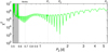 |
Fig. 12 Periodogram for the orbit of the third moon (S/2014 (130) 2). The χ2 values were computed from the 2014 astrometric data only, without contributions for other moons. The osculating period P2 was varied, while other elements were kept fixed. At the epoch T0 = 2457021.567880 (TDB), the synthetic position was very close to the observed one. The best-fit period is 1.642 days. For comparison, the period of 0.678 days from Berdeu et al. (2022) is indicated. |
4.6 Dynamical constraints for the oblateness
Having all three orbits, we performed a fitting of the oblateness C20 of the central body. We were interested not only in the best-fit model but also in poor fits, which enable us to reject the respective models. We computed an extended grid of models, with the oblateness C20 and the time lag Δt parameters kept fixed, while all other parameters were set free.
We included all multipole terms up to the order ℓ = 6 (from Table 3) in order to ensure that none of these high-order contributions to the total precession rate is missed. We also verified that orders ℓ > 6 only negligibly affect the value of χ2 Initial conditions for the simplex algorithm (Nelder & Mead 1965) must be set up precisely; in particular, P1,P2, and P3 must be close to the true or global minimum (for a given value of C20), otherwise the simplex could be ‘stuck’. We used two fully converged models for two different values of C20; we verified these minima are global by a χ2 mapping, knowing the typical spacing between the local minima, such as  , or
, or  , depending on the time span (2014 only, 2014–2019). Eventually, we determined the linear relations P1 (C20), P2(C20), and P3(C20), and interpolated the periods accordingly.
Overall, the best-fit model has  , with contributions
  ,
,  , and
, and  , where we used the weight wao = 0.3. All models are summarised in Fig. 13. The best-fit value of C20 ≃ −0.18, with an uncertainty of less than 0.01. This is slightly larger than the value computed for a homogeneous body.
Most importantly, we did not find any fits with C20 ≃ −0.16 that have lower or comparable χ2. On the contrary, the values were always significantly higher. This might be an indication of irregular, or (partially) differentiated internal structure; however, the irregularity should be more oblate, not more spherical.
Possible Elektra family. The nature of the meteorite analogue material (CM chondrites) and its average density (2.13 g cm−3) imply a substantial porosity of 28% for Elektra.
If these findings are accurate, a re-accumulation event might be at the origin of Elektra itself (and its satellite system). Usually, the event ends with a re-accumulation of streams (see e.g. Brož et al. 2022b), which deposit loose, low-dense, rubble-pile material, creating ‘hills’, some of which could be observed at the limb (see e.g. Fig. 5, top row, fifth column). Fragments from this event should also form a family. Even though there is no ‘official’ Elektra family (Nesvorný et al. 2015), (130) Elektra is embedded in the Alauda family ((702), FIN 9027). Given all of the arguments above, a part of this family should belong to Elektra; in particular, bodies with lower semimajor axis (a < 3.07 au), which do have similar inclinations to (130) Elektra (sin i ≃ 0.38).
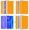 |
Fig. 13 Overview of best-fit models of the (130) system for the pair of fixed parameters: oblateness C20,1 and tidal time lag Δt1 (Brož et al. 2022a) of the central body. All other parameters were free. Each of the 147 models was converged for up to 1000 iterations, that is 147 000 models in total. The χ2 values are plotted as colours: cyan corresponds to the overall best fit, blue to good fits (1.2 times the best fit), orange to poor fits (1.5). The four panels correspond to the χ2 contributions: astrometry (SKY), relative astrometry of the moons (SKY2), silhouettes of the central body (AO), and the weighted sum of them. |
5 Conclusions
We present the first self-consistent model for all three moons of (130) Elektra. The model covers a considerably long time span (2014–2019) requiring a sufficiently complex dynamical model, including at least oblateness (ℓ = 2), which induces precession. With the constraint of three orbits and assuming a homogeneous internal structure, we obtain a precise mass for Elektra of  .
.
The relative astrometry of the moons seems more reliable than measurements with respect to (130) Elektra, because any possible issues with determining the photocentre of the primary are absent. The relative astrometry strongly suggests a dynamical oblateness of J2 ≃ 0.18, even with the high-order (ℓ = 6) multipoles included, which also contribute to the total precession. This higher oblateness would either require some internal structure or a substantial modification of the shape, ‘enforced’ by the observed precession. In the future, this should lead to new ‘photo-dynamical’ shape reconstruction methods.
Acknowledgements
The Czech Science Foundation supported this work through grants GA22-17783S (M.F., J.H.) and GA21-11058S (M.B.). In this work, measurements from the BlueEye600 telescope, supported by Charles University, were used.
Appendix A MCMC figures
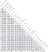 |
Fig. A.1 Corner plot showing the probability distributions of all parameters of the orbital model. Blue lines indicate a best-fit parameter, while the three dashed lines show the 16%, 50%, and 84% percentiles for each parameter. |
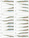 |
Fig. A.2 Markov chains. Each subplot corresponds to one variable and contains 33 walkers, each denoted by a different colour. Walkers, over 4000 iterations, mapped out possible values of the variables. |
Appendix B Observation data
In this Appendix, we present three tables of astrophotometry fits of the three moons of Elektra. In each table, x and y are the Cartesian positions of the moons relative to the photocentre of Elektra.
Astrophotometry fit of the inner moon S/2014 (130) 1.
Astrophotometry fit of the middle moon S/2014 (130) 2.
Astrophotometry fit of the outer moon S/2003 (130) 1.
Appendix C Extension of the best-fit orbital model
In this section, we present an extension of the best-fit orbital model from Sect. 4. There are several astrometric measurements of the outer moon S/2003, from 2003 to 2006, which were published in Marchis et al. (2008). To further test our best-fit model, we extended it by about 10 years into the past and added these older measurements. With some additional converging, the resulting model has a χ2 = 1406. In Fig. C.1, we present the fit of the outer moon’s orbit to the older positions.
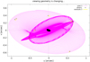 |
Fig. C.1 Extension of the best-fit quadrupole model, now with χ2 = 1406. Shown is only the relevant time span of 903 days for orbit 3. The orbit is plotted in the (u; v) coordinates (pink line), together with observed positions (black crosses), and residuals (yellow lines). The shape of Elektra for one of the epochs is overplotted in black. |
Appendix D Lightcurves
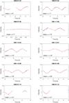 |
Fig. D.1 The light curves used in the shape reconstruction compared to the simulated light curves of the best-fit model. The observed intensity is represented by blue dots, while the simulated intensity of the shape model is depicted in red. The mean phase angle a for each observation is provided in the bottom left corner of each graph. |
References
- Benavidez, P. G., Durda, D. D., Enke, B. L., et al. 2012, Icarus, 219, 57 [NASA ADS] [CrossRef] [Google Scholar]
- Berdeu, A., Langlois, M., & Vachier, F. 2022, A & A, 658, A4 [Google Scholar]
- Brož, M. 2017, ApJS, 230, 19 [Google Scholar]
- Brož, M., Marchis, F., Jorda, L., et al. 2021, A & A, 653, A56 [Google Scholar]
- Brož, M., Ďurech, J., Carry, B., et al. 2022a, A & A, 657, A76 [Google Scholar]
- Brož, M., Ferrais, M., Vernazza, P., Ševeček, P., & Jutzi, M. 2022b, A & A, 664, A69 [Google Scholar]
- Claudi, R. U., Turatto, M., Gratton, R. G., et al. 2008, Ground-based and Airborne Instrumentation for Astronomy II, 7014, 1188 [Google Scholar]
- Devillard, N. 1997, The Messenger, 87, 19 [NASA ADS] [Google Scholar]
- Dohlen, K., Langlois, M., Saisse, M., et al. 2008, Ground-based and Airborne Instrumentation for Astronomy II, 7014, 1266 [Google Scholar]
- Durda, D. D., Bottke, W. F., Enke, B. L., et al. 2004, Icarus, 170, 243 [NASA ADS] [CrossRef] [Google Scholar]
- Ďurecti, J., Sidorin, V., & Kaasalainen, M. 2010, A & A, 513, A46 [Google Scholar]
- Ďurecti, J., Hanuš, J., Brož, M., et al. 2018, Icarus, 304, 101 [CrossRef] [Google Scholar]
- Foreman-Mackey, D., Hogg, D. W., Lang, D., & Goodman, J. 2013, PASP, 125, 306 [Google Scholar]
- Hanuš, J., Marchis, F., & Ďurech, J. 2013, Icarus, 226, 1045 [CrossRef] [Google Scholar]
- Hanuš, J., Marchis, F., Viikinkoski, M., Yang, B., & Kaasalainen, M. 2017, A & A, 599, A36 [Google Scholar]
- Levison, H. F., & Duncan, M. J. 1994, Icarus, 108, 18 [NASA ADS] [CrossRef] [Google Scholar]
- Marchis, F., Descamps, P., Berthier, J., et al. 2008, Icarus, 195, 295 [NASA ADS] [CrossRef] [Google Scholar]
- Nelder, J. A., & Mead, R. 1965, Comput, J, 7, 308 [CrossRef] [Google Scholar]
- Nesvorný, D., Brož, M., & Carruba, V. 2015, in Asteroids IV, 297 [Google Scholar]
- Park, R. S., Folkner, W. M., Williams, J. G., & Boggs, D. H. 2021, AJ, 161, 105 [NASA ADS] [CrossRef] [Google Scholar]
- Rivkin, A. S., Thomas, C. A., Howell, E. S., & Emery, J. P. 2015, AJ, 150, 198 [CrossRef] [Google Scholar]
- Robert, C., & Casella, G. 2011, Handbook of Markov Chain Monte Carlo, 49 [Google Scholar]
- Schmid, H. M., Bazzon, A., Roelfsema, R., et al. 2018, A & A, 619, A9 [NASA ADS] [CrossRef] [EDP Sciences] [Google Scholar]
- Si, H. 2006, TetGen, http://wias-berlin.de/software/tetgen/ [Google Scholar]
- Tierney, L. 1994, Ann. Stat., 22, 1701 [Google Scholar]
- Torppa, J., Hentunen, V.-P., Pääkkönen, P., Kehusmaa, P., & Muinonen, K. 2008, Icarus, 198, 91 [NASA ADS] [CrossRef] [Google Scholar]
- Vernazza, P., Marsset, M., Beck, P., et al. 2016, AJ, 152, 54 [CrossRef] [Google Scholar]
- Vernazza, P., Ferrais, M., Jorda, L., et al. 2021, A & A, 654, A56 [NASA ADS] [CrossRef] [EDP Sciences] [Google Scholar]
- Viikinkoski, M., Kaasalainen, M., & Ďurech, J. 2015, A & A, 576, A8 [Google Scholar]
- Vilas, F., & Gaffey, M. J. 1989, Science, 246, 790 [NASA ADS] [CrossRef] [Google Scholar]
- Yang, B., Wahhaj, Z., Beauvalet, L., et al. 2016, ApJ, 820, L35 [NASA ADS] [CrossRef] [Google Scholar]
i.e. not divided by N; the number of measurements.
Family Identification Number = 902 (Nesvorný et al. 2015).
All Tables
Summary of optical disk-integrated light curves of (130) Elektra obtained in this work by the BlueEye600 robotic observatory.
Multipole coefficients (up to ℓ = 6) of Elektra’s gravitational field derived from the ADAM shape, assuming homogeneous density.
All Figures
|
Fig. 1 Comparison of Elektra’s shape model to chords from occultation events. The red triangles represent the timing uncertainties at the ends of each chord and the dashed lines are non-detection chords. |
| In the text | |
|
Fig. 2 Best-fit shape model (top) and the alternative shape model (bottom) from three different viewing geometries. The first two are equator-on views rotated by 90° and the third one is a pole-on view. The model is lit up artificially to highlight its finer surface details. |
| In the text | |
|
Fig. 3 χ2 map for pole coordinates λ and β, where each value of χ2 is represented by a colour from the colour bar. The black tiles indicate values below the range of the colour bar, while the yellow tiles indicate values above the range of the colour bar. |
| In the text | |
|
Fig. 4 Distribution of Deq values based on shape models with χ2 values below 12. The 16%, 50%, and 84% percentiles of the distribution are shown with orange lines. |
| In the text | |
|
Fig. 5 AO images of Elektra (top), the best-fit shape model (middle), and the alternative shape model (bottom), all shown from the same viewing angle. The rotation axis is indicated by the red arrow. |
| In the text | |
|
Fig. 6 Keplerian model of orbits 1 and 3 with χ2 = 2195 over the time-span of 1707 days. The orbits are plotted in the (u; υ) coordinates (green and pink lines, respectively), together with observed positions (black crosses), and residuals (red and yellow lines, respectively). Elektra’s shape for one of the epochs is over-plotted in black. |
| In the text | |
|
Fig. 7 Quadrupole model of the orbits 1, 2, and 3 with χ2 = 1084 over the time-span of 1707 days. The orbits are plotted in the (u; υ) coordinates (green, blue and pink lines, respectively), together with observed positions (black crosses) and residuals (red, orange and yellow lines, respectively). Elektra’s shape for one of the epochs is overplotted in black. |
| In the text | |
|
Fig. 8 Same as Fig. 7, but plotted separately for each data set: Berdeu et al. (2022, top) and Vernazza et al. (2021, bottom). |
| In the text | |
|
Fig. 9 Evolution of the osculating elements of the inner moon S/2014 1 plotted over the time span of 1707 days. Shown is the semimajor axis a1, eccentricity e1, inclination i1, the longitude of the ascending node Ω1, and the longitude of the periapsis ϖ1. |
| In the text | |
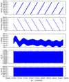 |
Fig. 10 Same as Fig. 9, but for the middle moon S/2014 2. |
| In the text | |
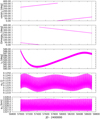 |
Fig. 11 Same as Fig. 9, but for the outer moon S/2003. |
| In the text | |
|
Fig. 12 Periodogram for the orbit of the third moon (S/2014 (130) 2). The χ2 values were computed from the 2014 astrometric data only, without contributions for other moons. The osculating period P2 was varied, while other elements were kept fixed. At the epoch T0 = 2457021.567880 (TDB), the synthetic position was very close to the observed one. The best-fit period is 1.642 days. For comparison, the period of 0.678 days from Berdeu et al. (2022) is indicated. |
| In the text | |
|
Fig. 13 Overview of best-fit models of the (130) system for the pair of fixed parameters: oblateness C20,1 and tidal time lag Δt1 (Brož et al. 2022a) of the central body. All other parameters were free. Each of the 147 models was converged for up to 1000 iterations, that is 147 000 models in total. The χ2 values are plotted as colours: cyan corresponds to the overall best fit, blue to good fits (1.2 times the best fit), orange to poor fits (1.5). The four panels correspond to the χ2 contributions: astrometry (SKY), relative astrometry of the moons (SKY2), silhouettes of the central body (AO), and the weighted sum of them. |
| In the text | |
|
Fig. A.1 Corner plot showing the probability distributions of all parameters of the orbital model. Blue lines indicate a best-fit parameter, while the three dashed lines show the 16%, 50%, and 84% percentiles for each parameter. |
| In the text | |
|
Fig. A.2 Markov chains. Each subplot corresponds to one variable and contains 33 walkers, each denoted by a different colour. Walkers, over 4000 iterations, mapped out possible values of the variables. |
| In the text | |
|
Fig. C.1 Extension of the best-fit quadrupole model, now with χ2 = 1406. Shown is only the relevant time span of 903 days for orbit 3. The orbit is plotted in the (u; v) coordinates (pink line), together with observed positions (black crosses), and residuals (yellow lines). The shape of Elektra for one of the epochs is overplotted in black. |
| In the text | |
|
Fig. D.1 The light curves used in the shape reconstruction compared to the simulated light curves of the best-fit model. The observed intensity is represented by blue dots, while the simulated intensity of the shape model is depicted in red. The mean phase angle a for each observation is provided in the bottom left corner of each graph. |
| In the text | |
Current usage metrics show cumulative count of Article Views (full-text article views including HTML views, PDF and ePub downloads, according to the available data) and Abstracts Views on Vision4Press platform.
Data correspond to usage on the plateform after 2015. The current usage metrics is available 48-96 hours after online publication and is updated daily on week days.
Initial download of the metrics may take a while.