| Issue |
A&A
Volume 649, May 2021
|
|
|---|---|---|
| Article Number | A83 | |
| Number of page(s) | 19 | |
| Section | Galactic structure, stellar clusters and populations | |
| DOI | https://doi.org/10.1051/0004-6361/202040026 | |
| Published online | 18 May 2021 | |
A KMOS survey of the nuclear disk of the Milky Way
I. Survey design and metallicities⋆,⋆⋆
1
Instituto de Astrofisica de Canarias, Calle Via Lactea s/n, 38205 La Laguna, Tenerife, Spain
e-mail: tobias.k.fritz@gmail.com
2
Universidad de La Laguna, Dpto. Astrofisica, 38206 La Laguna, Tenerife, Spain
3
Instituto de Astrofisica de Andalucia (CSIC), Glorieta de la Astronomia s/n, 18008 Granada, Spain
4
Max Planck Institute for extraterrestrial Physics, Giessenbachstraße 1, 85748 Garching, Germany
5
Max-Planck-Institut für Astronomie, Königstuhl 17, 69117 Heidelberg, Germany
6
The Department of Astronomy and Astrophysics, The University of Chicago, 5640 S. Ellis Ave., Chicago, IL 60637, USA
7
Laboratoire Lagrange, Université Côte d’Azur, Observatoire de la Côte d’Azur, CNRS, Blvd de l’Observatoire, Nice 06304, France
8
Research School of Astronomy & Astrophysics, Australian National University, ACT 2611, Australia
9
ARC Centre of Excellence for All Sky Astrophysics in Three Dimensions (ASTRO-3D), Australia
10
Departamento de Física Aplicada, Facultad de Ciencias, Universidad de Alicante, Carretera San Vicente s/n, 03690 San Vicente del Raspeig, Spain
Received:
30
November
2020
Accepted:
21
February
2021
Context. In the central few degrees of the bulge of the Milky Way there is a flattened structure of gas, dust, and stars, known as the central molecular zone, that is similar to nuclear disks in other galaxies. As a result of extreme foreground extinction, we possess only sparse information about the (mostly old) stellar population of the nuclear disk.
Aims. In this work we present our KMOS spectroscopic survey of the stars in the nuclear disk reaching the old populations. To obtain an unbiased data set, we sampled stars in the full extinction range along each line of sight.
Methods. We also observed reference fields in neighboring regions of the Galactic bulge. We describe the design and execution of the survey and present first results.
Results. We obtain spectra and five spectral indices of 3113 stars with a median S/N of 67 and measure radial velocities for 3051 stars. Of those, 2735 sources have sufficient S/N to estimate temperatures and metallicities from indices.
Conclusions. We derive metallicities using the CO 2-0 and Na I K-band spectral features, where we derive our own empirical calibration using metallicities obtained with higher-resolution observations. We use 183 giant stars for calibration spanning in metallicity from −2.5 to 0.6 dex and covering temperatures of up to 5500 K. The derived index based metallicities deviate from the calibration values with a scatter of 0.32 dex. The internal uncertainty of our metallicities is likely smaller. We use these metallicity measurements, together with the CO index, to derive effective temperatures using literature relations. We publish the catalog in this paper. Our data set complements Galactic surveys such as Gaia and APOGEE for the inner 200 pc radius of the Milky Way, which is not readily accessible by those surveys owing to extinction. We will use the derived properties in future papers for further analysis of the nuclear disk.
Key words: Galaxy: nucleus / Galaxy: abundances / Galaxy: kinematics and dynamics / catalogs / infrared: stars / techniques: spectroscopic
Table E.1 and Full Table D.1 are only available at the CDS via anonymous ftp to cdsarc.u-strasbg.fr (130.79.128.5) or via http://cdsarc.u-strasbg.fr/viz-bin/cat/J/A+A/649/A83
© ESO 2021
1. Introduction
The nuclear regions of galaxies show morphological and kinematic structures on scales of a parsec to a some hundred parsecs, which clearly set them apart from the large-scale structures of galaxies. Around the central black holes (Kormendy & Ho 2013) there are additional structures in stars, dust, and gas. On the scale of a few parsecs there are compact nuclear star clusters from 105 to a few 107 M⊙ (Böker et al. 2002; Walcher et al. 2005; Chatzopoulos et al. 2015b; Neumayer et al. 2020) in almost every galaxy with mass similar to that of the Milky Way. Further out, in spiral galaxies, particularly in barred spiral galaxies, there are more flattened structures such as nuclear rings, inner bars, and disks (Erwin & Sparke 2002; Launhardt et al. 2002; Comerón et al. 2010; Gadotti et al. 2019) of about a few 100 pc and up to 1 kpc (Gadotti et al. 2020)1. Often there is more dust and late star formation in the nuclear region than in the surrounding bulge and inner disk (Gadotti et al. 2019; Bittner et al. 2020).
Nuclear components are interesting on their own along with the way they are connected to the larger scales of a galaxy. Galactic centers are sinks of gas. In particular, bars move gas toward galactic centers. (Athanassoula et al. 1983; Binney et al. 1991; Emsellem et al. 2015). The gas accumulates at the inner Lindblad resonance of the bar and forms stars in that location (Athanassoula et al. 1983; Knapen 2005; Kim et al. 2012), often in rings. While the gas that is currently observed at the inner Lindblad resonance of the bar was probably only recently deposited, the stars keep an imprint of gas inflows that happened in the past. Star formation history can be used to infer how efficiently the bar transported gas to the center over time (Nogueras-Lara et al. 2019a; Bittner et al. 2020).
Further, a nuclear star formation burst may influence the outer galaxy through outflows (Veilleux et al. 2005) and form structures such as the Fermi bubble (Su et al. 2010), the radio bubble (Heywood et al. 2019), and the X-ray chimney (Ponti et al. 2019) in the Milky Way. In the other direction, compact structures such as globular clusters can migrate toward galactic centers owing to dynamic friction (Tremaine et al. 1975; Tsatsi et al. 2017) and deposit stars there. Such stars can be identified from their low metallicites (Dong et al. 2017). It is also possible that the nuclear cluster stars were formed locally or in locally formed clusters (Milosavljević 2004; Mastrobuono-Battisti et al. 2019).
All three nuclear components – the central black hole (Schödel et al. 2002), nuclear cluster (Becklin & Neugebauer 1968; Catchpole et al. 1990; Launhardt et al. 2002), and nuclear disk – exist together in the Milky Way, and are embedded into the bulge. In contrast to the bulge, there are young stars in clusters (Figer et al. 1999) and outside (Cotera et al. 1996, 1999; Clark et al. 2021) in the nuclear disk. There is also molecular gas called the central molecular zone (CMZ; Morris & Serabyn 1996; Mezger et al. 1996; Molinari et al. 2011; Kruijssen et al. 2015; Ginsburg et al. 2016), which has about the same extent as the stars of the nuclear disk (Launhardt et al. 2002). The nuclear cluster of the Milky Way has a size of about 5 pc (Fritz et al. 2016; Gallego-Cano et al. 2020). The nuclear disk has a radius of about 230 pc and a scale height of about 45 pc (Launhardt et al. 2002) and is similar but somewhat smaller than most extragalactic nuclear structures (Gadotti et al. 2019, 2020).
Comparing the chemistry of the oldest stars in the nuclear disk and the inner Galactic bulge (Ness et al. 2013; Schultheis et al. 2015; Zoccali et al. 2017) shows whether they are chemically similar. In that case the old nuclear disk stars are possibly (partly) just the inner continuation of the bulge, otherwise the stars are possibly connected to precursors of the current CMZ. There is an indication of differences between the nuclear cluster and the bulge (Nogueras-Lara et al. 2018a; Schultheis et al. 2019; Schödel et al. 2020). The bulge of the Milky Way is in its outer parts bar-shaped and mostly formed by secular evolution (Bland-Hawthorn & Gerhard 2016). However, it is still possible that an old classical bulge is hidden in the inner metal-poor bulge (Dékány et al. 2013; Kunder et al. 2020; Arentsen et al. 2020). The coverage of the inner bulge is still too limited to answer this question.
Photometric data of the nuclear disk are available from large-scale surveys. The most extensive bulge survey is Vista Variables in the Via Lactea (VVV) (Minniti et al. 2010). The Simultaneous-Color InfraRed Imager for Unbiased Survey (SIRIUS) covers the full nuclear disk and parts of the surrounding bulge (Nishiyama et al. 2013). GALACTICNUCLEUS (Nogueras-Lara et al. 2019b) also covers the central part of the nuclear disk at larger depth and sensitivity. The nuclear disk is much too extincted for Gaia proper motions (Gaia Collaboration 2018b). Hubble Space Telescope proper motions are now available in a relatively small area (Libralato et al. 2021), while crowding and saturation makes the larger area effort using VVV (Clarke et al. 2019) less useful. As a consequence of the large and variable extinction (Schödel et al. 2010; Fritz et al. 2011; Nogueras-Lara et al. 2018b), metallicity estimates based on color magnitude diagrams are difficult to obtain (Gonzalez et al. 2013); even J-band images are difficult to obtain at sufficient depth.
While the central few parsecs of the Milky Way have been already observed extensively with spectroscopic observations and high-resolution imaging (Genzel et al. 2010), the nuclear disk has not yet been studied in depth (Bland-Hawthorn & Gerhard 2016). The largest-scale work is radio based, consists of masers (Lindqvist et al. 1992; Trapp et al. 2018), and thus covers only a short and not well understood evolutionary phase. Outside the few known clusters, the nuclear cluster (Feldmeier et al. 2014; Do et al. 2015; Ryde et al. 2016; Fritz et al. 2016; Do et al. 2018; Thorsbro et al. 2020; Feldmeier-Krause et al. 2020; Davidge 2020) Arches and Quintuplet (Najarro et al. 2004; Martins et al. 2008; Clark et al. 2018a,b), near-infrared spectroscopy is limited, and was mostly aimed to target special stars such as young stellar objects (Nandakumar et al. 2018a), early-type stars with strong emission lines, and X-ray activity (Mauerhan et al. 2010a,b; Clark et al. 2021) or very red stars (Geballe et al. 2019). The most extensive data to date are likely from the APO Galactic Evolution Experiment (APOGEE) (Schönrich et al. 2015; Majewski et al. 2017; Schultheis et al. 2020). However, APOGEE is not ideal to study the Galactic nuclear disk. The relatively small telescope size and high extinction in the H-band limit the APOGEE observations and bias the sample to blue and intrinsically bright stars.
Therefore we executed a dedicated spectroscopic survey of the central 270 × 130 pc radius of the Milky Way targeting the nuclear disk and the innermost bulge in the IR − K-band using the K-band Multi Object Spectrograph (KMOS) (Sharples et al. 2013) at the Very Large Telescope (VLT). This paper is the first of a series. The paper is structured as follows: in Sect. 2 we describe our survey design and the obtained data. We detail the data reduction procedures in Sect. 3, including extraction of 1D spectra of the targets. We analyze the stellar spectra in Sect. 4 and measure the line-of-sight velocity and line index values. We use the latter to derive metallicities and effective temperatures in Sect. 5. This includes a new calibration for deriving metallicities from line indices. We give our summary and conclusions in Sect. 6.
2. Survey design
In this section we describe the design of our survey. First, we describe the general survey properties, and how we select the potential targets and fields for our KMOS observations. Finally, we describe the actually targeted stars and the observation setup.
2.1. General survey properties
Our dedicated survey of the nuclear disk has the following properties:
-
Our survey samples the full range of the nuclear disk (radius of ≈1.55° ≈220 pc and scale height of ≈0.3° ≈45 pc; see Launhardt et al. 2002) and line-of-sight depth to characterize the full nuclear disk.
-
Owing to the relatively small size (Launhardt et al. 2002; Nishiyama et al. 2013; Gallego-Cano et al. 2020), the line-of-sight distances of nuclear disk stars vary little. But there is a significant amount of dust in the nuclear region (Launhardt et al. 2002; Chatzopoulos et al. 2015a; Nogueras-Lara et al. 2020), which obscures stars at varying depth. For this reason, we selected our targets in extinction corrected magnitudes.
-
Our survey is designed to cover the full range in age and metallicity. The population with the faintest tip of the red giant branch (RGB) is old and metal-poor. Theoretical PARSEC isochrones (Bressan et al. 2012; Marigo et al. 2017) predict that the tip of the RGB of an old, metal-poor stellar population (12 Gyr, [Fe/H] = −1) is at MH = −6.09 and MK = −6.25. To reach the old stars of the nuclear disk, we selected predominantly stars that are fainter than this limit. The magnitude range of our sample extends over more than two magnitudes. Because of this, a small change in the extinction law over our fields does not affect the selected sample significantly. Further, metal-poor stars are bluer in (H − K) color. To prevent biases, we carefully selected stars distributed over the full range of (H − K) color in the nuclear disk.
We measured line-of-sight velocities of individual stars for dynamics. A relatively low resolution is sufficient to measure the internal dispersion of about 70 km s−1. Owing to the high extinction, temperatures need to be derived from spectra rather than from photometry. In future work, we will construct a Hertzsprung–Russell diagram with luminosities and temperatures to obtain the star formation history. We also determined metallicities for most stars. Because it is difficult to measure absolute properties, especially metallicities, we obtained the same kind of observations also outside the nuclear disk in the inner bulge. That way we can account for bulge pollution in our nuclear disk sample. Since the bulge is probably symmetric in star formation history and chemistry in latitude (Nandakumar et al. 2018b), sampling it on one side is sufficient.
The interstellar extinction toward the Galactic center is high (up to AK = 4.5, AH = 8 even when excluding infrared dark clouds). The magnitude of the tip of the RGB of old metal-poor stars and distance to the Galactic center of 8.18 kpc (Gravity Collaboration 2019) implies that stars fainter than mK = 12.8 or mH = 16.5 should be observed in a nuclear disk survey to sample the RGB tip completely. This H-band magnitude is far below the limit of APOGEE (Majewski et al. 2017) and is even challenging with H-band instruments at larger telescopes when more information than the line-of-sight velocity is wanted. Therefore, we observe exclusively in the K band.
2.2. Observed fields
We observe with the instrument KMOS (Sharples et al. 2013). The KMOS places 24 integral field units (IFUs) of 2.8″ × 2.8″ size over a diameter of 7.2′. The survey was executed in program 0101.B-0354 between April and September 2018. With the survey we target 24 fields in the nuclear disk and five reference fields in the bulge. Two bulge fields are located on both sides of the nucleus in the plane and three at increasing Galactic latitude at the same Galactic longitude as Sgr A*. We tried to sample the nuclear region evenly. We note that we avoided the inner few arcmin (the nuclear cluster) as it has been covered already by other programs (Fritz et al. 2016; Feldmeier-Krause et al. 2017, 2020). Not all requested fields in the central 0.2° region were observed (red circles in Fig. 1). In the central part we also placed some fields outside the midplane to be able to measure properties and gradients in scale height. In the outer parts where the nuclear disk is likely thinner (Launhardt et al. 2002) we only target it directly in the Galactic plane.
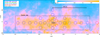 |
Fig. 1. Locations of the KMOS patrol fields of our survey. As shown by the colors, most were executed. Similar KMOS observations outside of this survey are also shown (Feldmeier-Krause et al. 2020, and in prep.). Together the full nuclear disk (Launhardt et al. 2002) is covered. The small black circle in the center shows the effective radius of the nuclear cluster (Gallego-Cano et al. 2020). The background shows a low-resolution extinction map in which the average extinction varies between AK = 0.45 and 2.93; see color bar. We made the extinction map from the catalog of Nishiyama et al. (2013). |
2.3. Target selection
We used 24 IFUs of KMOS for our target observations. As targets we selected stars primarily by K-band extinction corrected magnitude (K0). We targeted stars with K0 between 7 and 9.5. For a Galactic center distance of 8.18 kpc (Gravity Collaboration 2019) this corresponds to absolute magnitudes between −7.56 and −5.06. Thus, metal-poor old stars still fall within the selection window. Observationally, the extinction range extends from about AK = 0.5 (in the outermost bulge reference field) to about 4.5, which corresponds to observed magnitudes of mK = 7.5–15. As the primary catalog we used SIRIUS (Nagayama et al. 2003; Nishiyama et al. 2006). Compared to VVV (Minniti et al. 2010) and the Two Micron All Sky Survey (2MASS) (Skrutskie et al. 2006), SIRIUS has the advantage that neither saturation nor crowding affects the majority of our targets. We used VVV photometry where SIRIUS is not available. This affects two fields, in which about 12% are missing. Stars brighter than K = 9.2 are saturated in SIRIUS (see also Matsunaga et al. 2009); for these, we used 2MASS instead. This affects on average 3% of targets per field, but for the outer most bulge field, this rises to 30%. We aligned the 2MASS/VVV magnitude to SIRIUS by using the median of common sources to ensure that all stars are on the same calibration. We corrected for extinction on a star-by-star basis AK = (mH − mK − [(H − K)intr]) × 1.37; the factor is between Nishiyama et al. (2006) and the value of Fritz et al. (2011)2. For the intrinsic color ((H − K)intr), we used 0.25 as typical for bright giants.
We excluded stars that are clearly in front of the nuclear region to make our survey more efficient. Such foreground stars are less extinguished and thus more efficiently targeted with other spectrographs. We used a cut in H − K, which varies by field from 0.3 to 0.9. This is an intentionally blue color cut that aims to include all nuclear disk stars.
We probably included some foreground stars this way (Nogueras-Lara et al. 2019a), but it is easier to exclude an observed target a posteriori than to correct for missed stars. Using this color cut, on average we excluded 1% per field and at most 4%. In Schultheis et al. (2021) we used stricter cuts in color, which use spectroscopic information on star properties together with dynamic information to construct purer samples. Ultimately, the best approach is probabilistic, using all available information (i.e., colors, magnitudes, line-of-sight velocities, temperatures, and metallicities). After that step we made a selection by observed magnitude, we excluded sources with mK > 14, to limit the exposure time.
This magnitude selection effects only a few sources in the catalog, on average 0.1% per field, at most 0.7%. In practice there are probably more omitted very red sources because we omit stars which do not have H magnitudes from all catalogs. One reason for a missing H magnitude is that a source is too faint for detection. Similarly, a source can already be missing from the K-band catalog. To avoid a large impact from this, we shifted a few fields slightly to exclude lines of sight toward infrared dark clouds, for example, we shifted a field away from the symmetry axis to l/b −0.156/0.173° for that reason.
Since our program is designed for bad seeing, we excluded sources with a close neighbor3. We excluded a star when it has a close neighbor located within 2″ and < 0.5 mag fainter in K, within 2−2.5″ and > 0.5 mag brighter, or within 2.5−3″ and > 3 mag brighter. In total that results in the exclusion of 3%–18% (on average 9%) of the previously defined sources, depending mainly on source density, such that more sources are affected close to the Galactic center. Overall, our selection results in between 229 and 1283 main target stars per KMOS field. We added APOGEE sources within the fields for calibration. In total, there are 7 sources for the 29 patrol fields. Only 4 of those sources were actually observed because not all patrol fields were observed.
The details on the observations are in Appendix A. We show in Fig. 2 the CMD of our observed stars together with all stars in our field and the APOGEE targets in the inner Galaxy, all separated in nuclear disk and inner bulge4. For the star selection in nuclear disk and inner bulge we used shifted Galactocentric coordinates (l* and b*) such that Sgr A* is at 0/0. It is clear that toward the nuclear disk APOGEE only targets stars brighter than the old population or stars at extinctions clearly smaller than the mean. It is probably that nearly all of the latter are bulge stars projected onto the nuclear disk.
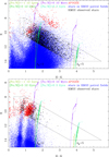 |
Fig. 2. Observed CMDs of nuclear disk based on SIRIUS/2MASS (top, |l*| < 1.55° and |b*| < 0.3°) and inner bulge (bottom |l*| < 2° and 0.3° < |b*| < 1°. There are two sequences in the KMOS bulge data because of the variable extinction (see also Nogueras-Lara et al. 2018a). In blue we show all stars within the KMOS fields. The KMOS and APOGEE target stars are shown in black and red, respectively. The shown isochrones are from PARSEC. The gray polygons outline our CMD selection of targets. The blue H − K color limit varies slightly from field to field. |
2.4. Design of the KMOS observing blocks
To observe a sufficiently large number of stars per field, we planned to observe five different KMOS configurations per field with varying targets distributed over the 24 KMOS arms. Therefore, we divided the above-defined catalog by K-band magnitude into five different subcatalogs. We used the K-band magnitude for reducing the dynamic range of each observing block (OB), to make it easier to avoid saturation and insufficient signal-to-noise (S/N). In the following, one such selection is called a subset. In part, not all subsets were observed successfully.
The targets were selected from the subcatalog with the arm allocation tool KARMA via the Hungarian algorithm. The number of potential targets is usually high enough that all arms can be allocated; in only a few cases 1–3 arms were not allocated. The algorithm results into an uneven spatial sampling, the center of a field (r < 1.4′) is targeted most densely, then there is a minimum at about 2.3′ from which it rises to the outer rim to nearly the same level as in the center. This effect is stronger with a larger catalog size. We show the effect in Fig. 3. For our science aims this uneven sample within a field is not important.
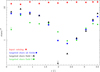 |
Fig. 3. Number of targets per square arcminute in a KMOS OB as a function of radial distance in arcminutes from the field center. The overall target numbers are divided by 24 to show the typical target density per KMOS field. Fields 1 and 5 are the most extreme fields in terms of target density: field 1 is at the higher density limit and field 5 is at the lower density limit and also has fewer observed stars because one subset was not successfully observed. The downward-facing arrows mark bins in which no star was observed. |
Because the stellar density is high in the Galactic center it was difficult to obtain an appropriate sky position for each individual OB (see, e.g., Feldmeier-Krause et al. 2017), even for such short exposures as those used in this work. Therefore, we observed a dedicated sky field centered on the dark cloud at l/b −0.0654/0.1575°. This ensured that we would encounter the minimal number of bright stars in each KMOS IFU in our sky fields. Three IFUs (18, 19, and 24) could not be allocated to a star-free sky area, and therefore we did not subtract any sky cube from these IFUs. The general subtraction of a spectrum constructed from nearly object free pixels in the science cube (see Sect. 3.3) acts as a first order sky correction. We check for the effect of missing sky cube subtraction in Appendix B.3.
For efficiency we do not dither for most targets and obtain only a single object and sky exposure. We only added some dithers for the lower extinction bulge fields since the lower exposure times make that possible. For the telluric data we used the standard observations provided by the observatory. These are observed with the standard three-arm telluric routine.
3. Data
In this section we present the procedure of reduction from raw data to 1D spectra. We present the data reduction, measure the quality of the cubes, and then extract the 1D spectra of the stars in the cubes. The details and potential problems of the spectra, OH lines and continuum ripples, are discussed in Appendix B.
3.1. Data reduction
We used close to the standard setting for most of our reduction, mainly with the software package SPARK (Davies et al. 2013). We changed the wavelength sampling to 3072 pixels (from 2048) to better sample the wavelength scale. For each day, we used the matching detector calibrations. We assigned the matching sky to the object OBs by hand, since the headers of our sky OBs have a science setting. We used the mode sky_tweak in the object file reduction step to optimally subtract the sky emission lines. Since we usually have only one exposure per target, cosmics are a problem. We corrected for them with LA-cosmic (van Dokkum 2001). We used the IDL variant for spectral cubes by Richard Davies5 and ran the script on the final cubes. The same code also creates the noise cubes, used in the following.
As our science goals require the analysis of various absorption features, a good correction of the telluric transmission is important. We used for the telluric correction, 31 standards observed in the nights of the science observations. We extracted spectra and noise spectra from the telluric cubes. We used all spatial pixels since the S/N is high and improves flux calibration. We treated each of the three spectrograph subsystem groups of IFUs (1–8, 9–16, 17–24) separately in the following because a different telluric spectrum is available for them. Our first sample includes all observed telluric standard stars besides the B emission line stars observed (HD 186456 and HD 171219). This sample consists mainly of early-type stars between B5V and A0V, one early white dwarf (HD2191), and three dwarfs between G0V and G2V. The spectrum of HD 194872, classified as G3V, looks like a colder spectral type and we thus exclude it, because such stars are difficult to model and are also too similar to the science targets. We first corrected the telluric spectra for the spectral features of the stars. For this, we used the ASPCAP model spectra (García Pérez et al. 2016) for the observed dwarfs of the same spectral types. We fit the best-fitting template to the observed spectra between 2.146 μm and 2.187 μm with the free parameters: normalization, velocity, and Gaussian smoothing width. By using this wavelength range we are concentrating on Brackett γ, the strongest line, but we check by eye that other lines are also well fitted. Before fitting we multiplied by the closest ATRAN (Lord 1992) model spectrum6 and eliminated any telluric affected wavelengths from the fit to avoid fitting the atmospheric features rather than the intrinsic spectral features. We required Gaussian smoothing to account for the strong rotation of early-type stars and the pressure-broadened white dwarf spectrum. For the G dwarfs no smoothing was necessary. We flux calibrated the corrected spectra using 2MASS magnitudes, black bodies matching the temperatures of the observed spectral types, and a flux of 4.288 × 10⁻¹⁰ W m−2 μm−1 for a magnitude of 0 at the reference wavelength of 2.157 μm. Between the different spectral types there is up to 5% ratio variation over the Ks band.
We did not use these transmission spectra directly because they often deviate too much in the atmospheric parameters (airmass and water vapor) from the science data. We used the telluric spectra to derive how each spectral pixel varies with airmass and with integrated water vapor. For the latter we used airmass times water vapor. For that we normalized all spectra, by taking the median of not strongly varying pixels. These pixels were identified in an iterative process, which gets more exclusive with the iterations. We then fit each spectral pixel with a linear model of airmass and integrated water vapor. This model is sufficient in general. It is not perfect when the transmission becomes nonlinear, which is the case for high airmass at wavelengths with low transmission, for example, around 2.02 μm. However, the flux is in any case so low that it cannot easily be used for analysis, thus the impact is minor. From the scatter of the 31 spectra compared to the fit we get the error. We find the median residual of the transmission is 1.3%, on average it is 1.5%, and at most 7%.
We then identified the telluric standard closest in atmospheric conditions to the science data. For that we determined the relative strength of the typical strength in airmass and water vapor. We find that the trend in airmass is four times stronger. Therefore we weight the airmass of science and tellurics up by a factor 4 and then chose the best match by calculating the distance in airmass-water vapor space to all and choosing the smallest one. We then changed that spectrum according to our linear model of airmass and water vapor to account for the airmass and water vapor differences between telluric and science observations.
3.2. Cube quality
Overall 24 of 29 fields were observed. In two fields (5 and 20) one of the five subsets was not observed. Two subsets in field 20 have a lower S/N, since the stars were not centered within the IFUs during acquisition. Owing to bad seeing in these fields, the stars extend into the IFUs and thus we still could extract spectra.
The first 10 observed subsets (fields 14 and 20) had one target less because arm 3 has not been active. The spatial resolution is usually good, although it is worst in field 20, where the full width at half maximum (FWHM) is about 1.3″ in the three subsets where the star center is in the IFUs, in the others it is difficult to determine. Excluding these fields, the FWHM is always less than 1″, and can be as low as 0.33″. We note that when the FWHM is so small, pixel digitization could impact this estimate. Overall the median FWHM is 0.57″.
3.3. Star spectra extraction
We extracted the stellar spectra using a dedicated spectral extraction routine, which subtracts a local background before extraction of the object spectrum. This is important because the background stellar emission of similar sources can lead to an underestimation of the dispersion (Lützgendorf et al. 2015). Also in case of several sources, a more targeted extraction is necessary in an IFU. We collapsed the (non-telluric corrected) cubes into an average image and worked with this image using the approach explained below. We started with extraction of the pixels of the primary object. This is identified by the brightest pixel. We fit the point spread function (PSF) shape by a 2D Gaussian using a 3 pixel radius box around it. We used the Gaussian fit to identify the pixels with more than 50% of the maximum stellar flux; they represent our usual estimate of object pixels. With the 50% limit, we achieved maximum S/N for most noise regimes and PSF shapes. If that methods results in 3 or less pixels we added the next brightest pixels, until we obtained 4 pixels. Thus, we avoided an undersampled PSF, which leads to strong ripples in the continuum (see also Appendix B.2). If the Gaussian PSF fit failed, we used pixel count ordering. Neighboring pixels were first checked to see whether they are above the flux cut. Then all pixels were checked to see whether they have at least 50% of the flux of the brightest pixel. For the background, we simply used the faintest pixels of the collapsed cube. We used at least 25% of all pixels. This number is increased, when the object covers many pixels to avoid that the overall S/N is limited by the background. The same background pixels are used for secondary sources. Secondary sources are local maxima compared to all neighboring pixels, which are not within a primary source or the background and have sufficient S/N. The S/N cut is chosen such that essentially all sources for which spectral features are detectable are included. However, we did not include all sources that were detectable in the continuum. At most three secondary sources were found per IFU. We then added pixels from the surrounding ring of pixels when the following conditions were fulfilled: They are not already selected for a source or background and they are brighter than 50% of the main secondary pixel.
After that first extraction, we carried out three quality control checks on the primary sources to make sure that they are the targets selected from the catalog.
-
Firstly, we compared the spectroscopic flux and spectroscopic color against the photometric properties from the input catalog. We also checked the sources for which the primary source has less than 50% of the flux of all sources in the cube.
-
Secondly, we checked the target pixel coordinates against the typical target pixel coordinates in the other IFUs in that exposure to identify offset sources.
-
Lastly, we also checked all sources whose S/N is below 10.
When one of these three checks has a negative outcome we looked at the collapsed cube and, if the current extraction was clearly suboptimal, we changed object pixels by hand. For a few collapsed IFU cubes we also identified additional secondary sources during that process. In case of sources with more than one exposure, we also ensured that the order of sources is always the same. For some sources we saw in the collapsed cubes that the background include bad pixels. All these changes affected only 37 sources (i.e., 1.2% of all targets).
4. Spectroscopic analysis
In this section we describe how we measure basic properties from the spectra. We measure the line-of-sight velocity and spectral indices for H2O, Brackett γ, Na I, Ca I, and CO 2-0.
4.1. Velocity measurements
As a first step we obtained radial velocities because they are needed for the subsequent analysis of the spectra. Most stars show CO band heads, and we used cross-correlation at 2.18−2.425 μm to measure line-of-sight velocities because the band heads are too complex for other ways of analysis. We normalized our spectra to 1 by fitting linear function to the spectra before the CO band heads (2.08 μm–2.29 μm). As templates we used GNIRS spectra from Gemini7, which cover at least from 2.18 μm to 2.425 μm. We selected mostly very late giants and some earlier giants between F7 and M0. For most stars the best correlation is achieved with the K7III star, HD63425B. We correlated all KMOS spectra with all templates. Usually very similar velocities are achieved for all the different templates. Then we correlated the template with the largest correlation coefficient in wavelength sections with the spectra. In most cases, we selected six sections: one before the band heads and then one for each band head. In all but 43 cases the velocities in the different sections agree very well. The others we inspected more closly; a few are clearly late-type but have positive spikes (and a few negative ones) likely due to sky subtraction problems. We corrected them like bad pixels. Further, we correlated the problematic spectra in three sections: one before and two in the band heads. After that process all except for 19 of the primary spectra have a velocity consistently determined over the full wavelength range and in sections, with at most 30 km s−1 difference and usually much less. The velocities also show a small scatter (at most 45 km s−1) between the different sections and their velocities are also in agreement for the different templates. We inspected the more divergent cases by eye. These are all late-type stars. Thus, velocities with large errors can also be trusted, since there is the right signal in the spectra.
In total we have 3405 CO based velocities of primary spectra. Not all are from different stars, since some stars have several exposures. For the velocity errors (σl.o.s.) we primarily used the error given by the correlation. This is usually consistent with the scatter from the velocities determined in sections, although the latter should be larger when the error is dominated by S/N. That shows that we are not underestimating errors and that for most stars the S/N does not matter for the error, but systematics like template target mismatch are the dominating contributions. For stars with S/N < 25, the formal correlation errors are larger. We corrected for that to obtain the velocity error over the full range by ![$ \sigma_{\mathrm{l.o.s.\,segm}}=\sqrt{\sigma_{\mathrm{segm}}^2-(c/[{S/N}])^2} $](/articles/aa/full_html/2021/05/aa40026-20/aa40026-20-eq1.gif) , where σsegm is the scatter over the velocities in the different wavelength ranges, and c is determined such that σl.o.s. segm is in the median the same as the error of the correlation over the full wavelength range. We compared the errors obtained this way with the errors obtained by correlation. We used the errors obtained in this way for stars that have a large σl.o.s. segm (less than 5% likelihood by chance). That is the case for 248 spectra. We used the same method for secondary source spectra.
, where σsegm is the scatter over the velocities in the different wavelength ranges, and c is determined such that σl.o.s. segm is in the median the same as the error of the correlation over the full wavelength range. We compared the errors obtained this way with the errors obtained by correlation. We used the errors obtained in this way for stars that have a large σl.o.s. segm (less than 5% likelihood by chance). That is the case for 248 spectra. We used the same method for secondary source spectra.
Stars in some bulge fields have several exposures. We combined their measurements in the following way. We only used exposures that have a velocity measurement. Of these, we combined the different velocities error weighted. In the median the error derived from the error weighted scatter over the different exposures is consistent with the error that follows from the error weighted combination of the individual uncertainties. We checked for each star whether the χ2 is within the 95% quantile for the available number of spectra. That is the case for 201 stars, and not for 44 stars. For these, we upscaled the error by  The upscale factor is at most 3.6 and the final uncertainty at most 17 km s−1, which shows that our statistical errors are estimated well and small. Their S/N is calculated as
  .
.
Overall we have CO-based velocities for 2790 primary sources and for 241 secondary sources. We obtain velocities for the early-type stars by fitting their lines (see Patrick et al., in prep.). For the primary sources, there are six spectra without velocity, of which five have low S/N below 12 and one has a higher S/N and is feature free. We discuss these more in Patrick et al. (in prep.), together with the other young stars. Of the stars with CO lines the median velocity error is 2.5 km s−1, the 5% with the largest error have errors larger than 6 km s−1, the 1% with the largest error have errors larger than 11 km s−1, and the largest error is 44 km s−1. Secondary sources perform somewhat worse, as expected due to the lower S/N: Of these, 40 spectra have no velocity, of which 33 have low S/N below 24 and 7 have higher S/N, and are some kind of early-type star. Of the secondary stars with CO lines the median velocity error is 4.5 km s−1, 5% with the largest error have errors larger than 20 km s−1, and the largest error is 54 km s−1. We test the velocity calibration and errors (see Appendix C) and make small corrections based on these errors. An overall shift of 4 km s−1 for the velocities and we set a lower limit of 4.2 km s−1 for the error. We show the velocities as a function Galactic longitude in Fig. 4.
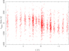 |
Fig. 4. Barycentric velocities of all stars with measurements as a function of Galactic longitude. |
4.2. Spectroscopic indices
We measured the spectroscopic indices for Brackett γ, Na I, Ca I, CO 2-0, and H2O for all stars. To obtain the wavelengths in the reference frame of each star, we used the velocity previously determined without barycentric corrections. For stars without a velocity measurement, we assume a velocity of 0. The wavelength ranges for the indices are summarized in Table 1.
Vacuum wavelength ranges used for the spectroscopic indices.
For the CO index we used the index definition of Frogel et al. (2001)8. For the continuum reference we fit the four continuum ranges by a linear function in which we give all ranges the same weight. We then integrated over the CO band range without interpolation and converted the result to the equivalent width (EW) in Å. We estimated the error from repeated observations of the same star. It is 57/(S/N). This could be an underestimation when systematics such as extinction or velocity play a role. The index of Frogel et al. (2001) is not particularly sensitive to those (Pfuhl et al. 2011), but a small contribution is possible.
For Brackett γ we constructed our own index (see Table 1). For this index we obtained an error of 23/(S/N) from repeated observations of the same star. We also calculated the Na I and Ca I indices of Frogel et al. (2001) for our stars. From the repeat observations we estimated an error of 27/(S/N) for the Na index and of 58/(S/N) for the Ca index. We show these indices as a function of CO, which is a good approximation for effective temperature, in Fig. 5.
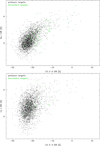 |
Fig. 5. Na (top) and Ca (bottom) as a function of CO index. For Na all stars with an S/N > 20 are shown; the value where the intrinsic scatter of CO and Na is of the size of the measurement error. For Ca the S/N is lower and thus only stars with an S/N > 40 are plotted. |
We show in Fig. 6 the CO and Brackett γ indices. Even when all (including low S/N) stars are plotted, the expected structure is visible. Most stars have strong CO absorption and essentially no Brackett γ absorption or emission, thus EWBr γ ≈ 0. These stars are too cold for hydrogen lines. Moving to weaker CO there is then weak Brackett γ absorption. When the index is larger than about −4 Å most high S/N stars have no CO based velocity. These are the young stars (see Patrick et al., in prep.). Around EWCO ≈ −5 Å several stars have weak CO absorption and narrow Brackett γ absorption, which is expected for warm stars. They are not early-type stars (Habibi et al. 2019). Finally, we look at stars with an CO EW index more negative than −4 Å to find stars unusual in Brackett γ, which have CO. We only look at stars with an S/N > 20. We determine the median in bins and fit a quadratic function to it. We then look at stars that deviate by more than 2 Å from the track. For some of them the signal is spurious. However, we find three genuinely unusual stars.
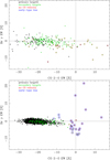 |
Fig. 6. CO and Brackett γ equivalent widths for all stars. Stars with early-type lines are confirmed with visual inspection of the spectra. In the top panel the stars with an S/N < 20 are shown; in the bottom panel the stars with an S/N > 20 are shown. This S/N is the approximately border of the nearly complete regime of spectral classification. The lines divide absorption (negative) and emission. |
We checked whether or not these and all stars are asymptotic giant branch (AGB) stars. Therefore, we looked for broad H2O features as typical for AGB stars (see, e.g., Lançon & Wood 2000). Because our spectra only cover the K band, we cannot construct the usual indices, which require H and K coverage such as in Blum et al. (2003). We constructed our own index by fitting the continuum between 2.18 and 2.291 μm (excluding Na and Ca features) with a linear function of log λ. This is the wavelength range at which neither H2O nor CO has features. The extrapolation of the fit gives the expected continuum. Then we measured the H2O in a full width window of 0.014 μm around 1.992 μm. This is the bluest wavelength range at which the atmospheric transmission is still acceptable. This and all other index windows are shown in Fig. 7.
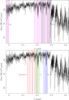 |
Fig. 7. Index windows together with a typical spectrum. The continuum windows are shown hatched, the feature windows cross hatched. The spectrum is typical for a primary target spectrum in S/N and CO and Na index values. In the top panel the molecular indices are shown; in the bottom panel the atomic indices are shown. |
The ratio of this flux and the extrapolated continuum flux gives the H2O index. We checked the formal error by analyzing the stars with multiple exposures. We find that the error is underestimated for higher S/N. The main reason is not clear but effects like correlated errors and imperfect telluric correction could be responsible. We add to the formal errors 0.048 in quadrature to have realistic errors over the full S/N range.
We checked the H2O index for dependence on extinction, by determining the median index in extinction bins. We excluded stars with K0 < 7.5 because there are many AGB stars and thus there is a stronger variation. There is a trend over the full range, but the impact over the central 80% extinction range (AK between 1.46 and 3.49) is 0.044 smaller than the error floor; it steepens somewhat at the blue and red end. The H2O index is smaller for more extincted stars. That is expected when the stars are not all at the same distance since more distant stars suffer higher extinction and are intrinsically brighter. Brighter stars have a larger H2O index in our sample in the median. Whether this can explain the full trend is unclear. It is possible that we do not fully correct for extinction effects in our measurement. It is also possible that our assumption of constant (H − K)0 = 0.25 matters. Still, the index is sufficiently well determined so that plausible trends are visible (see Fig. 8). Most stars, including the early-type stars, have an index between 0.8 and 1.1; 153 stars have an index below 0.7 and are strong candidates for AGB stars. They are distributed over a relatively large range in CO index between −8 and −32 EW [Å]. The 3 late-type stars with Brackett γ emission are among them and belong to the AGB candidates with the weakest CO features. A similar trend is visible in the figure S13 of Lançon & Wood (2000), which is for the same star in different phases. These stars also belong to the brightest in our sample, but the luminosity could be slightly overestimated since we do not consider AGB star effects for the effective temperature and intrinsic color estimation.
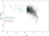 |
Fig. 8. H2O index as a function of extinction corrected magnitude K0 for stars with S/N > 20. Unusual sources are indicated with open symbols, blue circles (early-type or young stellar objects), or boxes (AGB with Brackett γ). Sources with H2O index below 0.7 are probably AGB stars. |
5. Physical properties
To obtain physical properties of the late-type stars (all stars with CO absorption and radial velocity measurements) we used the indices. We used calibration stars with known metallicity to derive an index-metallicity relation. For temperatures, we combined CO index-temperature relations from the literature.
5.1. Metallicity calibration
Firstly, to estimate the metallicity, we tested the index calibrations of Frogel et al. (2001). Frogel et al. (2001) collected a sample of calibrators together with their Na, Ca, and CO equivalent widths and fit the full sample with linear and quadratic functions. We find that both their options lead to unrealistic low metallicities for stars with strong lines. The quadratic function even leads to decreasing metallicity for stronger Na at large CO EW depth. That is not surprising because the calibration of Frogel et al. (2001) is based on globular clusters and thus is not well suited for the expected metallicity range of our sample. We therefore derived our own calibration. We used Na and CO EW widths because they have the highest S/N. Frogel et al. (2001) found that Ca contributes only weakly to the metallicity estimate. We also find a weak metallicity sensitivity of Ca.
5.1.1. Metallicity index construction
For the derivation of our own calibration we used the following spectra.
-
Firstly, 18 of our KMOS stars were also observed by APOGEE and have their metallicity determined in DR16 (Ahumada et al. 2020).
-
Secondly, we used the X-shooter spectral library (XSL), precisely the spectra published in Gonneau et al. (2020). We selected spectra with log(g) < 2.5 according to Arentsen et al. (2019). Around the order transition at 2.275 μm the XSL spectra show some spikes, we corrected for the worst by assigning them bad pixels. Also we calculated an alternative CO index that uses two continuum points redward of the problematic region. The two CO indices deviated from each other by 1.0 Å EW standard deviation with a median bias of 0.5 Å EW, whereby the Frogel et al. (2001) index is slightly smaller. We used the average of both in the following. A few stars have several spectra in the XSL. We compared the values obtained for these and found the differences are very small, and thus they measure the same quantities. In such cases we used the median of the index values by excluding stars with a positive (CO emission) CO index because we only analyzed stars with CO absorption in this work. Thirdly, we used SINFONI spectra of the Galactic center stars from Thorsbro et al. (2020). For GC25 we did not have a spectrum and we excluded GC16867 because of too small S/N. A few stars have two spectra with very similar EW values. Therefore we used their average.
-
Finally, we also used NGC 6583−46 for which we obtained a spectrum with FIRE9.
For stellar properties we used APOGEE DR16 properties when possible. We used [Fe/H] when available and used [M/H], as provided by Ahumada et al. (2020), for three KMOS stars for which [Fe/H] is not available. From the stars with both, we determined that [M/H] is on average 0.012 dex larger, we subtracted this number from three metal-rich stars that do not have [Fe/H]. The APOGEE data are available for the 18 KMOS stars and for 21 stars from XSL. For these stars we determined that the average difference in metallicity between APOGEE and Arentsen et al. (2019) is 0.088 dex, whereas the metallicity of APOGEE is larger. Therefore, we added 0.088 dex to all metallicities from Arentsen et al. (2019). For the Galactic center stars we used the [Fe/H] from Thorsbro et al. (2020). We used for NGC 6583−46 the high-resolution spectroscopy results of Magrini et al. (2010) for this cluster. In general these different data sets agree about as well as expected from their errors. The exception is that cold stars from Arentsen et al. (2019) do not follow the same pattern in CO−Na space; the Co−Na space pattern is more random in latter work. Arentsen et al. (2019) mention in Sect. 5.4 that they do not trust their results below 3800 K, therefore we excluded those stars.
From all samples we excluded stars brighter than MK = −7.5. We chose this limit since the nuclear disk stars sample excludes brighter stars and because beyond that limit most stars are not red giants, rather AGB stars and supergiants, which often have different index strengths for the same temperature. We used Gaia DR2 parallaxes (Gaia Collaboration 2018b) for the local stars, and a Galactic center distance of 8.18 kpc (Gravity Collaboration 2019; Bland-Hawthorn & Gerhard 2016) for the bulge and nuclear stars. Similarly, we used distances from Harris (1996) for the globular cluster stars and a distance of 50.1 kpc and 62.8 kpc for the Large and Small Magellanic Cloud member stars, respectively (Fritz et al. 2020). For NGC 2324 we used a distance of 3.8 kpc (Piatti et al. 2004) and for NGC 2682 we use da distance of 0.88 kpc (Gaia Collaboration 2018a). For magnitudes we used for most, 2MASS. Besides we used the previously mentioned SIRIUS magnitudes for the KMOS stars and magnitudes from Fritz et al. (2016) for the stars from Thorsbro et al. (2020). We corrected the latter stars like the nuclear stars for extinction. We did not correct the others for extinction; the extinction is usually small and does not matter much that we included a few stars that are slighly brighter because not all of these stars have different indices. We excluded stars with H2O-index < 0.7, which excludes most AGB stars.
All this together results in a sample of 187 stars, which are listed in Appendix D. We tried to fit the full sample at once, but found that such a high order polynomial is needed, that extrapolation beyond the data range is implausible, and also that within the data the metallicity does not always increase with feature strength in contrast to the expectations. Therefore we divided the data set into parts by CO strengths. Firstly, there is a shallow CO depth range, that is, the part where the maximum possible Na strength does not increase much. That is the case for EWCO > −11.5 Å (see top of Fig. 9). Secondly, this is a region where the Na and CO EWs clearly vary. We chose a range down to CO EW of −8.5 Å to make sure both use, in part, the same data, which avoids a big jump in the overlap region. When applied to spectra we linearly changed the weight of the two for EW between −11 and −9 to ensure a smooth overlap. We excluded four outliers from the sample, two of which are of very low CO depth, where we do not derive metallicities from targets.
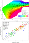 |
Fig. 9. Metallicity derivation. Top: calibration of metallicity based on CO and Na EW. The large symbols represent the 183 used calibration spectra; the symbol shape shows the source of spectra and metallicity (Magrini et al. 2010; Thorsbro et al. 2020; Ahumada et al. 2020; Arentsen et al. 2019). The value is indicated by the color within SINF indicates SINFONI. The background shows the derived relation; the color range saturates below [Fe/H] < −2.5 and above [Fe/H] > 0.6 (the range of the calibrators.), where the derived values are based on more uncertain extrapolation. The two vertical lines separate the application of the high and low CO solutions; in the overlap region in between both high and low CO solutions are used to derive metallicities. The small dots show all our KMOS targets with S/N > 30 and a CO based velocity. The background shows the derived value only for areas where either calibrators or the nuclear stars have coverage. Bottom: comparison between literature (x-axis) and our metallicities (y-axis). The thick black line indicates the identity line; the thin lines bracket the typical uncertainty. Stars are coded by CO depth; the hottest have the smallest depth. |
We derive the following relation. For EWCO > −8.5 we obtain
![$$ \begin{aligned} \mathrm{[Fe/H]}&=-3.14-0.0106\,\mathrm{EW} _\mathrm{CO} -1.98\,\mathrm{EW} _\mathrm{Na} +0.00763\,\mathrm{EW} _\mathrm{CO} ^2\nonumber \\&\quad -0.0929\,\mathrm{EW} _\mathrm{CO} \,\mathrm{EW} _\mathrm{Na} +0.00646\,\mathrm{EW} _\mathrm{Na} ^2 , \end{aligned} $$](/articles/aa/full_html/2021/05/aa40026-20/aa40026-20-eq4.gif)
wherein all EW are in Å. For EWCO < −11.5 we obtain
![$$ \begin{aligned} \mathrm{[Fe/H]}&=-1.65+0.0317\,\mathrm{EW} _\mathrm{CO} -1.07\,\mathrm{EW} _\mathrm{Na} +0.00195\,\mathrm{EW} _\mathrm{CO} ^2\nonumber \\&\quad -0.0288\,\mathrm{EW} _\mathrm{CO} \,\mathrm{EW} _\mathrm{Na} -0.0211\,\mathrm{EW} _\mathrm{Na} ^2 . \end{aligned} $$](/articles/aa/full_html/2021/05/aa40026-20/aa40026-20-eq5.gif)
In the bottom panel of Fig. 9 we show the comparison between the metallicities of our reference sample and our derived metallicities using Eqs. (1) and (2). We note that the scatter is larger for the warmest stars with the weakest CO absorption, which is expected because for those stars the used features are weak. The standard deviation between the input and the derived [Fe/H] is 0.32, which varies little over almost the entire range of CO depth. The scatter is 0.5 for EWCO > −2. It does not impact our conclusions because none of our targets stars has such a small depth; the smallest depth of a late-type star in our science sample is −2.5 when ignoring low S/N sources.
We see in addition more deviations from the identity line for metal-rich stars ([Fe/H] > 0). This is because cool metal-rich giants (Teff < 4000 K) suffer from substantial molecular lines in their spectra, which results in consequent line blending and blanketing and affects the stellar parameters. The increased scatter could therefore also be due to the larger errors in the metallicities of the reference sample we are using. Of our sample, 72% are cool stars with EW < −20, which lie mostly inside the 1σ scatter. In the top panel of Fig. 9, it is visible that the metallicity follows the expectations: the metallicity increases with increasing Na depth for constant CO.
The deviation between input and derived metallicity probably has several contributions. The S/N caused error is small for most stars, which is clear from repeated observations of the same star. At shallow CO depth, S/N can contribute; the continuum problem of the XSL spectra can also contribute. The error in the calibrator [Fe/H] is small for APOGEE (in median 0.013 and at most 0.036) and NGC 6583−46 (0.08); in addition for the stars of Thorsbro et al. (2020) the error is 0.15, which is still small compared to the uncertainty in this work. From the overlap of Arentsen et al. (2019) and APOGEE we derive an uncertainty of 0.09, which is consistent with their median error of 0.08. Thus, all these errors are small. That is also confirmed when we compare the scatter by spectra/metallicity calibration: all are within 1σ of each other when the stars with EWCO > −2 are excluded. The different data sets show somewhat different offsets, the main XSL (Arentsen et al. 2019) agrees not surprisingly, since it dominates the fit. Surprisingly the XSL APOGEE sample has an offset of −0.2 dex with respect to the model. Since this sample consists mainly of globular clusters, this may show that they are somewhat different in these indicators. Because there are not so many nuclear disk stars in their [Fe/H] range it does not influence the results much. The SINFONI-Thorsbro et al. (2020) sample has an offset of −0.1 dex with respect to the model. That is because the mean metallicity of this sample is smaller than that of most nuclear samples, which are summarized in Schultheis et al. (2019). Not surprisingly, the APOGEE-KMOS sample has an offset of 0.1 dex with respect to the model, since the model selects a compromise between the APOGEE-KMOS and SINFONI-Thorsbro et al. (2020) samples that dominate the low temperature end. This difference shows that our metallicity calibration has an uncertainty of about 0.1 dex.
5.1.2. Application of the metallicity index
We now apply the index to our target stars. To check the impact of the calibration, we also calculated [Fe/H], excluding either SINFONI-Thorsbro et al. (2020) or KMOS-APOGEE from the fit and the other samples are always used. The indices of our spectra have errors that cause metallicity uncertainties. We calculated the resulting metallicity error via a Monte Carlo (MC) simulation; we assumed a Gaussian distribution of the EW values and calculated the metallicity for 10 000 random realizations. From the MC samples we calculated the 1σ confidence intervals. In the median this value is 0.13 dex, which is small compared to the calibration error. This depends mostly on the S/N of the spectra, but the strength of the CO and Na indices also matters because for strong indices, [Fe/H] varies less per Å. For EWCO < −15, we find that the error is typically σ[Fe/H] = 0.93/(S/N). For the smallest CO depth, the error is a factor 4 larger. Because metal-poor stars usually have shallower CO depths, their random error is usually larger. We provide the errors in the result table (see Appendix E). Depending on the application, these errors can be used on their own or when the calibration error is added. The former is the case when rather similar stars are compared and only relative metallicity matters, the latter when the stars are rather different or the absolute metallicity matters.
The obtained numbers confirm that the S/N cannot be the main reason for the 0.32 dex scatter in the calibration sample. One reason for this could be that we used the [Fe/H] of the spectra, but we did not measure Fe Our indices measure mainly Na and C10. We looked into that possibility by using the APOGEE stars, in it 33 stars have [C/Fe] and 24 have [Na/Fe], the latter is rarely available for the most metal-rich stars. For Na we did not find a trend in [Fe/H]index–[Fe/H]APOGEE nor did we find this trend when we divided the sample into XSL and KMOS spectra to account for the different offsets11. We find weak trends for [C/Fe]. We find a trend slope of 1.19 ± 0.95 for the APOGEE-KMOS sample and a trend slope of 0.28 ± 0.26 (0.34 ± 0.26 excluding one outlier) for the APOGEE-XSL sample, where a slope of 1.0 would fully explain the offset. Thus, while abundance variations are probably not enough to explain the full error they likely contribute. This is because there is no trend in [Na/Fe] could be because this index measures not only Na but also Sc I for cold stars (see, e.g., Park et al. 2018). We show the metallicity distribution of our survey stars in Fig. 10.
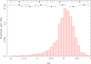 |
Fig. 10. Metallicity distribution of survey stars. All 2734 stars with CO absorption and S/N > 30 are shown. At the top, the median statistical error of stars passing these cuts are indicated in black and in blue the calibration uncertainty, which does not depend on metallicity. |
5.2. Temperature calibration
Another property that can be obtained from spectra of our resolution is the temperature. For the cool stars that dominate our sample, a common method is to use the CO band heads. It is often assumed that their strength depends only on the temperature (see, e.g., Blum et al. 2003; Schultheis et al. 2016; Feldmeier-Krause et al. 2017). The strength also depends, however, on the metallicity, at least for metallicities clearly below solar (see, e.g., Frogel et al. 2001 and Mármol-Queraltó et al. 2008). To estimate the temperature we used the calibration of Mármol-Queraltó et al. (2008). This calibration uses as input our CO EW and our metallicity. When the metallicity is outside the range of −2.5 to 0.6, we set it to the closer limit. The range combines the range of the calibrators of Mármol-Queraltó et al. (2008) and of our calibrators. For low temperatures, Mármol-Queraltó et al. (2008) calibrated with relatively few stars, which likely causes the following problem. Below about 3290 K the temperature increases slightly toward lower Na EW for constant CO, which is the opposite of what is expected (Frogel et al. 2001). Therefore we used the relation of Feldmeier-Krause et al. (2017) for very large CO depths; this relation does not depend on metallicity. We corrected for the offset between the two scales by subtracting 50 K from the Feldmeier-Krause et al. (2017) values, which is the difference between the two scales for solar metallicity at 3290 K. We used only Mármol-Queraltó et al. (2008) for COEW > −21.5 and only Feldmeier-Krause et al. (2017) adjusted for COEW < −22.5. In between we transitioned linearly between the two. The use of Feldmeier-Krause et al. (2017) also has the advantage that only very few stars are extremely cold. We show the temperature as a function of indexes EW in Fig. 11.
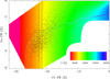 |
Fig. 11. Temperature calibration for stars with CO absorption. For CO EW larger than −21.5 Å, the equations of Mármol-Queraltó et al. (2008) are used. These equations use our [Fe/H] determination. Below −22.5 the calibration by Feldmeier-Krause et al. (2017), corrected for the offset between the two, is used. Between these values (indicated by the two black lines) there is a linear transition between the two relations. The diagonal strip shows the uncorrected relation by Feldmeier-Krause et al. (2017). It is plotted for |[Fe/H]| < 0.075. The color scales saturate outside of 2600 K and 5800 K. The dots show our KMOS targets with S/N > 30. |
For solar metallicity, the two scales are relatively similar, with the Mármol-Queraltó et al. (2008) based temperatures being usually about 100 K lower than the Feldmeier-Krause et al. (2017) based temperatures. However, there are also differences of up to 200 K for high temperatures12. We calculated the temperature errors caused by S/N for all stars in a MC simulation. In that simulation we included the effects of metallicity uncertainties. The median uncertainty is 64 K for primary sources and 284 K for secondary sources. The difference is mostly caused by the higher S/N of the primary sources. Other parameters have some impact as well. There is an error minimum around 3600 K. Those errors are usually an underestimate. The calibration of Feldmeier-Krause et al. (2017) has a residual scatter of 163 K and the calibration of Mármol-Queraltó et al. (2008) of 32 K. For the calibration used, as well for other temperature calibrations (Pfuhl et al. 2011; Schultheis et al. 2016; Feldmeier-Krause et al. 2017), we find that the resulting median temperature for solar metallicity stars is cooler than all possible temperatures from PARSEC (Bressan et al. 2012) and BaSTI (Pietrinferni et al. 2004) isochrones for stars with MK > −6. This could indicate a problem with isochrones or a problem with the effective temperatures. The latter could be affected by differences between spectroscopic and photometric temperatures; spectroscopic temperatures can be calibrated (Jönsson et al. 2020; González Hernández & Bonifacio 2009) on photometric but that is difficult especially for relatively cool stars. In both cases this shows the limitations of past star formation histories obtained from spectroscopy such as Blum et al. (2003), Pfuhl et al. (2011). We give CO based temperatures for all stars with CO based velocities and negative EWCO and also for stars with EWCO < −4 without velocity because such a depth occurs only for late-type stars (see Fig. 6).
We cannot estimate a temperature for stars without CO absorption in this way. We provide rough estimates based on the lines present. We assume a temperature of 10 000 K for stars that show only Brackett γ absorption and a temperature of 25 000 K for stars that also, or only, show lines with higher ionization potential. We assign an intermediate temperature of 8000 K to all other stars (most of them of low S/N). We show the temperature distribution in Fig. 12. It is visible that while M-giants dominate the sample, it also contains warmer stars of different spectral classes.
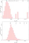 |
Fig. 12. Temperature distribution of survey stars. The spectral class (borders) are indicated in the top of the plots. Top panel: all stars with S/N > 20, that is, all stars that were classifiable (with a single exception). The latter is grouped together with the young stellar objects at 8000 K. This temperature and that of the hotter stars is qualitative based on spectral feature existence. Bottom panel: zoom-in of the colder stars (stars with CO absorption) with S/N > 30, for which temperatures from line indices are calculated. |
We estimate from the temperatures the intrinsic H − K color for better extinction estimates. We use PARSEC 3.3 isochrones (Bressan et al. 2012; Chen et al. 2014, 2015; Tang et al. 2014; Marigo et al. 2017; Pastorelli et al. 2019) for the conversion from effective temperatures to H − K colors. We round our metallicities to one decimal and set limits of −2.5 dex and 0.6 dex. We download isochrones in 0.1 dex steps between −2.5 dex and 0.6 dex for 30 Myr, 1 Gyr and 12 Gyr. We use stars from MK = 2 (to exclude dwarfs which follow a different track) to the tip of the RGB because later phases are less well modeled. We also exclude stars warmer than 5600 K because our stars are cooler. For all the selected data points we fit the H − K points with a fourth order polynomial of the temperature. The data points deviate at most by 0.014 mag in the standard deviation from these fits, likely other uncertainties such as model or passband uncertainties are more important. We extrapolate to lower temperatures by using the linear slope at the coolest data point; 21% of the stars are in the extrapolation regime. We set stars colder than 2700 K to this temperature because no giants in PARSEC are cooler and these temperatures are likely caused by uncertainties. Using the PARSEC isochrones, we assign to the hot stars (8000 K, 10 000 K, and 25 000 K) colors of H − K0 = 0.01, −0.01 and H − K0 = −0.09. Overall our targets have an average intrinsic color H − K0 of 0.30 with a scatter of 0.07; within the error consistent with our input assumption of always 0.25.
We use these intrinsic H − K colors to order the targets in H-K corrected for the intrinsic color (H − K0). All stars are compared with all potential target stars (see Sect. 2.3) in that field, that is, the stars that have magnitudes between K0 = 7 and K0 = 9.5. For unobserved target stars, we draw the intrinsic color using the mean and standard deviation of the primary targets with S/N > 30 in that field. Since in field 20 most stars have low S/N, we use the average of the four neighboring fields. The extinction ordering parameter ext-order is defined as the fraction of stars which has an H − K0 smaller than the target star. Ext-order orders by extinction because stellar effects are corrected for. Ext-order is mainly an estimate for the line-of-sight order, although extinction variation in the plane of sky of the fields contributes as well. Ext-order is published in our catalog (see Appendix E).
6. Summary and conclusions
In this paper we introduce our spectroscopic survey of the nuclear disk. This region is highly extincted, limiting Gaia and even APOGEE observations. The aim of the presented survey is to study the older stellar populations in the nuclear disk region, which have not been previously systematically studied. Therefore, we target stars with absolute extinction-corrected magnitudes below the tip of the RGB of old stars. Even though we do not use color selection criteria, most (more than 99%) observed stars are red giants because they are the most abundant stars in the observed magnitude range.
We observe 20 fields in the nuclear disk and four reference fields in the nearby inner bulge with the multi-object IFU instrument KMOS/VLT. We obtain K-band spectra of 3113 stars with a median S/N of 67. We measure velocities for 3051 stars with a typical accuracy of 5 km s−1. We measure line indices of Brackett γ, Na, Ca, CO 2-0, and H2O to identify contaminants (AGB, young stars) and to measure physical properties of late-type stars. We find 2735 sources have sufficient S/N to estimate temperatures and metallicities that are limited by systematics. We measure metallicities using the two strongest features of cool (≤5500 K) stars in the K band: CO and Na. For calibration we use 183 giants with metallicities between −2.5 dex and 0.6 dex obtained with higher-resolution observations and K-band spectra. The resulting metallicities deviate from the calibration values with a scatter of 0.32 dex. The internal uncertainties of our metallicities are likely smaller, since the uncertainty caused by S/N has a median value of 0.13 dex and we observe mostly similar luminosity stars. We obtain temperatures from CO using the literature relations of Mármol-Queraltó et al. (2008) and Feldmeier-Krause et al. (2017).
Our data also contain a number of early-type stars. In addition to hot stars, which display only hydrogen, the data include stars with lines with higher ionization potential and a few young stellar objects. We will publish a detailed analysis of the young stars and other rare stars in Patrick et al. (in prep.). These sources are also included in our catalog. We are publishing the catalog in electronic form at the CDS along with this paper. We already analyzed (Schultheis et al. 2021) the metallicity properties and its dependence on other properties, particularly dynamics, similar to Schultheis et al. (2020) for APOGEE data covering the inner bulge and the nuclear disk. In the future we will utilize the velocities and metallicities to constrain the nuclear disk mass and dynamic state, and improve existing measurements for nuclear disk (Sormani et al. 2020) and nuclear cluster (Chatzopoulos et al. 2015b). Further, we will study the star formation history of the nuclear disk (similar to Blum et al. 2003; Pfuhl et al. 2011 for the nuclear cluster), and test if the majority of stars of the nuclear disk are indeed old (Nogueras-Lara et al. 2019a).
We note that more recent works get slightly smaller factors; see Nogueras-Lara et al. (2018b, 2020).
For APOGEE we used all of the published sources in DR16 (Ahumada et al. 2020), which besides the main survey targets also includes telluric targets and targets of other observations. Aside from the outlined spatial selection, we required K magnitude and S/N > 14. Below this number even line-of-sight velocities are often unreliable.
C is limiting in CO, see Frogel et al. (2001).
However, we note that Na belongs to the least reliable elements in APOGEE; see Jönsson et al. (2020).
Both differences are for the unadjusted Feldmeier-Krause et al. (2017) scale.
Acknowledgments
This research made use of Astropy (http://www.astropy.org), a community-developed core Python package for Astronomy (Astropy Collaboration 2013, 2018). This work has made use of data from the European Space Agency (ESA) mission Gaia (https://www.cosmos.esa.int/gaia), processed by the Gaia Data Processing and Analysis Consortium (DPAC, https://www.cosmos.esa.int/web/gaia/dpac/consortium). Funding for the DPAC has been provided by national institutions, in particular the institutions participating in the Gaia Multilateral Agreement. This paper includes data gathered with the 6.5 m Magellan Telescopes located at Las Campanas Observatory, Chile. Author R. S. acknowledges financial support from the State Agency for Research of the Spanish MCIU through the “Center of Excellence Severo Ochoa” award for the Instituto de Astrofísica de Andalucía (SEV-2017-0709). RS acknowledges financial support from national project PGC2018-095049-B-C21 (MCIU/AEI/FEDER, UE). N. N. and F. N.-L. gratefully acknowledge support by the Deutsche Forschungsgemeinschaft (DFG, German Research Foundation) – Project-ID 138713538 – SFB 881 (‘The Milky Way System’, subproject B8).
References
- Ahumada, R., Allende Prieto, C., Almeida, A., et al. 2020, ApJS, 249, 3 [CrossRef] [Google Scholar]
- Arentsen, A., Prugniel, P., Gonneau, A., et al. 2019, A&A, 627, A138 [NASA ADS] [CrossRef] [EDP Sciences] [Google Scholar]
- Arentsen, A., Starkenburg, E., Martin, N. F., et al. 2020, MNRAS, 491, L11 [CrossRef] [Google Scholar]
- Astropy Collaboration (Robitaille, T. P., et al.) 2013, A&A, 558, A33 [NASA ADS] [CrossRef] [EDP Sciences] [Google Scholar]
- Astropy Collaboration (Price-Whelan, A. M., et al.) 2018, AJ, 156, 123 [Google Scholar]
- Athanassoula, E., Bienayme, O., Martinet, L., & Pfenniger, D. 1983, A&A, 127, 349 [NASA ADS] [Google Scholar]
- Becklin, E. E., & Neugebauer, G. 1968, ApJ, 151, 145 [NASA ADS] [CrossRef] [Google Scholar]
- Binney, J., Gerhard, O. E., Stark, A. A., Bally, J., & Uchida, K. I. 1991, MNRAS, 252, 210 [NASA ADS] [CrossRef] [Google Scholar]
- Bittner, A., Sánchez-Blázquez, P., Gadotti, D. A., et al. 2020, A&A, 643, A65 [CrossRef] [EDP Sciences] [Google Scholar]
- Bland-Hawthorn, J., & Gerhard, O. 2016, ARA&A, 54, 529 [NASA ADS] [CrossRef] [EDP Sciences] [Google Scholar]
- Blum, R. D., Ramírez, S. V., Sellgren, K., & Olsen, K. 2003, ApJ, 597, 323 [NASA ADS] [CrossRef] [Google Scholar]
- Böker, T., Laine, S., van der Marel, R. P., et al. 2002, AJ, 123, 1389 [NASA ADS] [CrossRef] [Google Scholar]
- Bressan, A., Marigo, P., Girardi, L., et al. 2012, MNRAS, 427, 127 [NASA ADS] [CrossRef] [Google Scholar]
- Catchpole, R. M., Whitelock, P. A., & Glass, I. S. 1990, MNRAS, 247, 479 [NASA ADS] [Google Scholar]
- Chatzopoulos, S., Gerhard, O., Fritz, T. K., et al. 2015a, MNRAS, 453, 939 [NASA ADS] [CrossRef] [Google Scholar]
- Chatzopoulos, S., Fritz, T. K., Gerhard, O., et al. 2015b, MNRAS, 447, 948 [Google Scholar]
- Chen, Y., Girardi, L., Bressan, A., et al. 2014, MNRAS, 444, 2525 [NASA ADS] [CrossRef] [Google Scholar]
- Chen, Y., Bressan, A., Girardi, L., et al. 2015, MNRAS, 452, 1068 [NASA ADS] [CrossRef] [Google Scholar]
- Churchwell, E., Babler, B. L., Meade, M. R., et al. 2009, PASP, 121, 213 [NASA ADS] [CrossRef] [Google Scholar]
- Clark, J. S., Lohr, M. E., Najarro, F., Dong, H., & Martins, F. 2018a, A&A, 617, A65 [CrossRef] [EDP Sciences] [Google Scholar]
- Clark, J. S., Lohr, M. E., Patrick, L. R., et al. 2018b, A&A, 618, A2 [NASA ADS] [CrossRef] [EDP Sciences] [Google Scholar]
- Clark, J. S., Patrick, L. R., Najarro, F., Evans, C. J., & Lohr, M. E. 2021, A&A, 649, A43 [EDP Sciences] [Google Scholar]
- Clarke, J. P., Wegg, C., Gerhard, O., et al. 2019, MNRAS, 489, 3519 [NASA ADS] [CrossRef] [Google Scholar]
- Comerón, S., Knapen, J. H., Beckman, J. E., et al. 2010, MNRAS, 402, 2462 [NASA ADS] [CrossRef] [Google Scholar]
- Cotera, A. S., Erickson, E. F., Colgan, S. W. J., et al. 1996, ApJ, 461, 750 [NASA ADS] [CrossRef] [Google Scholar]
- Cotera, A. S., Simpson, J. P., Erickson, E. F., et al. 1999, ApJ, 510, 747 [NASA ADS] [CrossRef] [Google Scholar]
- Davidge, T. J. 2020, AJ, 160, 146 [Google Scholar]
- Davies, R. I., Agudo Berbel, A., Wiezorrek, E., et al. 2013, A&A, 558, A56 [NASA ADS] [CrossRef] [EDP Sciences] [Google Scholar]
- Dékány, I., Minniti, D., Catelan, M., et al. 2013, ApJ, 776, L19 [NASA ADS] [CrossRef] [Google Scholar]
- Do, T., Kerzendorf, W., Winsor, N., et al. 2015, ApJ, 809, 143 [NASA ADS] [CrossRef] [Google Scholar]
- Do, T., Kerzendorf, W., Konopacky, Q., et al. 2018, ApJ, 855, L5 [NASA ADS] [CrossRef] [Google Scholar]
- Dong, H., Schödel, R., Williams, B. F., et al. 2017, MNRAS, 471, 3617 [NASA ADS] [CrossRef] [Google Scholar]
- Emsellem, E., Renaud, F., Bournaud, F., et al. 2015, MNRAS, 446, 2468 [NASA ADS] [CrossRef] [Google Scholar]
- Erwin, P., & Sparke, L. S. 2002, AJ, 124, 65 [NASA ADS] [CrossRef] [Google Scholar]
- Feldmeier, A., Neumayer, N., Seth, A., et al. 2014, A&A, 570, A2 [NASA ADS] [CrossRef] [EDP Sciences] [Google Scholar]
- Feldmeier-Krause, A., Neumayer, N., Schödel, R., et al. 2015, A&A, 584, A2 [NASA ADS] [CrossRef] [EDP Sciences] [Google Scholar]
- Feldmeier-Krause, A., Kerzendorf, W., Neumayer, N., et al. 2017, MNRAS, 464, 194 [NASA ADS] [CrossRef] [Google Scholar]
- Feldmeier-Krause, A., Kerzendorf, W., Do, T., et al. 2020, MNRAS, 494, 396 [CrossRef] [Google Scholar]
- Figer, D. F., Kim, S. S., Morris, M., et al. 1999, ApJ, 525, 750 [NASA ADS] [CrossRef] [Google Scholar]
- Fritz, T. K., Gillessen, S., Dodds-Eden, K., et al. 2011, ApJ, 737, 73 [NASA ADS] [CrossRef] [Google Scholar]
- Fritz, T. K., Chatzopoulos, S., Gerhard, O., et al. 2016, ApJ, 821, 44 [NASA ADS] [CrossRef] [Google Scholar]
- Fritz, T. K., Di Cintio, A., Battaglia, G., Brook, C., & Taibi, S. 2020, MNRAS, 494, 5178 [Google Scholar]
- Frogel, J. A., Stephens, A., Ramírez, S., & DePoy, D. L. 2001, AJ, 122, 1896 [NASA ADS] [CrossRef] [Google Scholar]
- Gadotti, D. A., Sánchez-Blázquez, P., Falcón-Barroso, J., et al. 2019, MNRAS, 482, 506 [Google Scholar]
- Gadotti, D. A., Bittner, A., Falcón-Barroso, J., et al. 2020, A&A, 643, A14 [CrossRef] [EDP Sciences] [Google Scholar]
- Gaia Collaboration (Babusiaux, C., et al.) 2018a, A&A, 616, A10 [NASA ADS] [CrossRef] [EDP Sciences] [Google Scholar]
- Gaia Collaboration (Brown, A. G. A., et al.) 2018b, A&A, 616, A1 [NASA ADS] [CrossRef] [EDP Sciences] [Google Scholar]
- Gallego-Cano, E., Schödel, R., Nogueras-Lara, F., et al. 2020, A&A, 634, A71 [CrossRef] [EDP Sciences] [Google Scholar]
- García Pérez, A. E., Allende Prieto, C., Holtzman, J. A., et al. 2016, AJ, 151, 144 [Google Scholar]
- Geballe, T. R., Lambrides, E., Schlegelmilch, B., et al. 2019, ApJ, 872, 103 [NASA ADS] [CrossRef] [Google Scholar]
- Genzel, R., Eisenhauer, F., & Gillessen, S. 2010, Rev. Mod. Phys., 82, 3121 [Google Scholar]
- Ginsburg, A., Henkel, C., Ao, Y., et al. 2016, A&A, 586, A50 [NASA ADS] [CrossRef] [EDP Sciences] [Google Scholar]
- Gonneau, A., Lyubenova, M., Lançon, A., et al. 2020, A&A, 634, A133 [NASA ADS] [CrossRef] [EDP Sciences] [Google Scholar]
- Gonzalez, O. A., Rejkuba, M., Zoccali, M., et al. 2013, A&A, 552, A110 [NASA ADS] [CrossRef] [EDP Sciences] [Google Scholar]
- González Hernández, J. I., & Bonifacio, P. 2009, A&A, 497, 497 [NASA ADS] [CrossRef] [EDP Sciences] [Google Scholar]
- Gravity Collaboration (Abuter, R., et al.) 2019, A&A, 625, L10 [NASA ADS] [CrossRef] [EDP Sciences] [Google Scholar]
- Habibi, M., Gillessen, S., Pfuhl, O., et al. 2019, ApJ, 872, L15 [CrossRef] [Google Scholar]
- Harris, W. E. 1996, AJ, 112, 1487 [NASA ADS] [CrossRef] [Google Scholar]
- Heywood, I., Camilo, F., Cotton, W. D., et al. 2019, Nature, 573, 235 [CrossRef] [Google Scholar]
- Jönsson, H., Holtzman, J. A., Allende Prieto, C., et al. 2020, AJ, 160, 120 [CrossRef] [Google Scholar]
- Kim, W.-T., Seo, W.-Y., Stone, J. M., Yoon, D., & Teuben, P. J. 2012, ApJ, 747, 60 [NASA ADS] [CrossRef] [Google Scholar]
- Knapen, J. H. 2005, A&A, 429, 141 [NASA ADS] [CrossRef] [EDP Sciences] [Google Scholar]
- Kormendy, J., & Ho, L. C. 2013, ARA&A, 51, 511 [Google Scholar]
- Kruijssen, J. M. D., Dale, J. E., & Longmore, S. N. 2015, MNRAS, 447, 1059 [NASA ADS] [CrossRef] [Google Scholar]
- Kunder, A., Pérez-Villegas, A., Rich, R. M., et al. 2020, AJ, 159, 270 [Google Scholar]
- Lançon, A., & Wood, P. R. 2000, A&AS, 146, 217 [NASA ADS] [CrossRef] [EDP Sciences] [Google Scholar]
- Launhardt, R., Zylka, R., & Mezger, P. G. 2002, A&A, 384, 112 [NASA ADS] [CrossRef] [EDP Sciences] [Google Scholar]
- Libralato, M., Lennon, D. J., Bellini, A., et al. 2021, MNRAS, 500, 3213 [Google Scholar]
- Lindqvist, M., Habing, H. J., & Winnberg, A. 1992, A&A, 259, 118 [NASA ADS] [Google Scholar]
- Lord, S. D. 1992, A New Software Tool for Computing Earth’s Atmospheric Transmission of Near- and Far-Infrared Radiation (NASA Technical Memorandum 103957) [Google Scholar]
- Lützgendorf, N., Gebhardt, K., Baumgardt, H., et al. 2015, A&A, 581, A1 [NASA ADS] [CrossRef] [EDP Sciences] [Google Scholar]
- Magrini, L., Randich, S., Zoccali, M., et al. 2010, A&A, 523, A11 [NASA ADS] [CrossRef] [EDP Sciences] [Google Scholar]
- Majewski, S. R., Schiavon, R. P., Frinchaboy, P. M., et al. 2017, AJ, 154, 94 [NASA ADS] [CrossRef] [Google Scholar]
- Marigo, P., Girardi, L., Bressan, A., et al. 2017, ApJ, 835, 77 [NASA ADS] [CrossRef] [Google Scholar]
- Mármol-Queraltó, E., Cardiel, N., Cenarro, A. J., et al. 2008, A&A, 489, 885 [NASA ADS] [CrossRef] [EDP Sciences] [Google Scholar]
- Martins, F., Hillier, D. J., Paumard, T., et al. 2008, A&A, 478, 219 [NASA ADS] [CrossRef] [EDP Sciences] [Google Scholar]
- Mastrobuono-Battisti, A., Perets, H. B., Gualandris, A., Neumayer, N., & Sippel, A. C. 2019, MNRAS, 490, 5820 [CrossRef] [Google Scholar]
- Matsunaga, N., Kawadu, T., Nishiyama, S., et al. 2009, MNRAS, 399, 1709 [NASA ADS] [CrossRef] [MathSciNet] [Google Scholar]
- Mauerhan, J. C., Cotera, A., Dong, H., et al. 2010a, ApJ, 725, 188 [NASA ADS] [CrossRef] [Google Scholar]
- Mauerhan, J. C., Muno, M. P., Morris, M. R., Stolovy, S. R., & Cotera, A. 2010b, ApJ, 710, 706 [NASA ADS] [CrossRef] [Google Scholar]
- Mezger, P. G., Duschl, W. J., & Zylka, R. 1996, A&ARv, 7, 289 [NASA ADS] [CrossRef] [Google Scholar]
- Milosavljević, M. 2004, ApJ, 605, L13 [NASA ADS] [CrossRef] [Google Scholar]
- Minniti, D., Lucas, P. W., Emerson, J. P., et al. 2010, New Astron., 15, 433 [Google Scholar]
- Molinari, S., Bally, J., Noriega-Crespo, A., et al. 2011, ApJ, 735, L33 [NASA ADS] [CrossRef] [Google Scholar]
- Morris, M., & Serabyn, E. 1996, ARA&A, 34, 645 [NASA ADS] [CrossRef] [Google Scholar]
- Nagayama, T., Nagashima, C., Nakajima, Y., et al. 2003, in Instrument Design and Performance for Optical/Infrared Ground-based Telescopes, eds. M. Iye, & A. F. M. Moorwood, SPIE Conf. Ser., 4841, 459 [Google Scholar]
- Najarro, F., Figer, D. F., Hillier, D. J., & Kudritzki, R. P. 2004, ApJ, 611, L105 [NASA ADS] [CrossRef] [Google Scholar]
- Nandakumar, G., Schultheis, M., Feldmeier-Krause, A., et al. 2018a, A&A, 609, A109 [NASA ADS] [CrossRef] [EDP Sciences] [Google Scholar]
- Nandakumar, G., Ryde, N., Schultheis, M., et al. 2018b, MNRAS, 478, 4374 [NASA ADS] [CrossRef] [Google Scholar]
- Ness, M., Freeman, K., Athanassoula, E., et al. 2013, MNRAS, 430, 836 [Google Scholar]
- Neumayer, N., Seth, A., & Böker, T. 2020, A&ARv, 28, 4 [CrossRef] [Google Scholar]
- Nishiyama, S., Nagata, T., Kusakabe, N., et al. 2006, ApJ, 638, 839 [Google Scholar]
- Nishiyama, S., Yasui, K., Nagata, T., et al. 2013, ApJ, 769, L28 [NASA ADS] [CrossRef] [Google Scholar]
- Nogueras-Lara, F., Schödel, R., Dong, H., et al. 2018a, A&A, 620, A83 [NASA ADS] [CrossRef] [EDP Sciences] [Google Scholar]
- Nogueras-Lara, F., Gallego-Calvente, A. T., Dong, H., et al. 2018b, A&A, 610, A83 [NASA ADS] [CrossRef] [EDP Sciences] [Google Scholar]
- Nogueras-Lara, F., Schödel, R., Gallego-Calvente, A. T., et al. 2019a, Nat. Astron., 4, 377 [Google Scholar]
- Nogueras-Lara, F., Schödel, R., Gallego-Calvente, A. T., et al. 2019b, A&A, 631, A20 [NASA ADS] [CrossRef] [EDP Sciences] [Google Scholar]
- Nogueras-Lara, F., Schödel, R., Neumayer, N., et al. 2020, A&A, 641, A141 [EDP Sciences] [Google Scholar]
- Park, S., Lee, J.-E., Kang, W., et al. 2018, ApJS, 238, 29 [Google Scholar]
- Pastorelli, G., Marigo, P., Girardi, L., et al. 2019, MNRAS, 485, 5666 [Google Scholar]
- Pfuhl, O., Fritz, T. K., Zilka, M., et al. 2011, ApJ, 741, 108 [NASA ADS] [CrossRef] [Google Scholar]
- Piatti, A. E., Clariá, J. J., & Ahumada, A. V. 2004, A&A, 418, 979 [NASA ADS] [CrossRef] [EDP Sciences] [Google Scholar]
- Pietrinferni, A., Cassisi, S., Salaris, M., & Castelli, F. 2004, ApJ, 612, 168 [NASA ADS] [CrossRef] [Google Scholar]
- Ponti, G., Hofmann, F., Churazov, E., et al. 2019, Nature, 567, 347 [NASA ADS] [CrossRef] [Google Scholar]
- Ryde, N., Fritz, T. K., Rich, R. M., et al. 2016, ApJ, 831, 40 [NASA ADS] [CrossRef] [Google Scholar]
- Schödel, R., Ott, T., Genzel, R., et al. 2002, Nature, 419, 694 [NASA ADS] [CrossRef] [PubMed] [Google Scholar]
- Schödel, R., Najarro, F., Muzic, K., & Eckart, A. 2010, A&A, 511, A18 [NASA ADS] [CrossRef] [EDP Sciences] [Google Scholar]
- Schödel, R., Nogueras-Lara, F., Gallego-Cano, E., et al. 2020, A&A, 641, A102 [CrossRef] [EDP Sciences] [Google Scholar]
- Schönrich, R., Aumer, M., & Sale, S. E. 2015, ApJ, 812, L21 [NASA ADS] [CrossRef] [Google Scholar]
- Schultheis, M., Cunha, K., Zasowski, G., et al. 2015, A&A, 584, A45 [NASA ADS] [CrossRef] [EDP Sciences] [Google Scholar]
- Schultheis, M., Ryde, N., & Nandakumar, G. 2016, A&A, 590, A6 [NASA ADS] [CrossRef] [EDP Sciences] [Google Scholar]
- Schultheis, M., Rich, R. M., Origlia, L., et al. 2019, A&A, 627, A152 [NASA ADS] [CrossRef] [EDP Sciences] [Google Scholar]
- Schultheis, M., Rojas-Arriagada, A., Cunha, K., et al. 2020, A&A, 642, A81 [EDP Sciences] [Google Scholar]
- Schultheis, M., Fritz, T. K., Nandakumar, G., et al. 2021, A&A, in press, https://doi.org/10.1051/0004-6361/202140499 [Google Scholar]
- Sharples, R., Bender, R., Agudo Berbel, A., et al. 2013, The Messenger, 151, 21 [NASA ADS] [Google Scholar]
- Skrutskie, M. F., Cutri, R. M., Stiening, R., et al. 2006, AJ, 131, 1163 [NASA ADS] [CrossRef] [Google Scholar]
- Sormani, M. C., Magorrian, J., Nogueras-Lara, F., et al. 2020, MNRAS, 499, 7 [Google Scholar]
- Spitzer Science Center 2009, VizieR Online Data Catalog: II/293 [Google Scholar]
- Su, M., Slatyer, T. R., & Finkbeiner, D. P. 2010, ApJ, 724, 1044 [NASA ADS] [CrossRef] [Google Scholar]
- Tang, J., Bressan, A., Rosenfield, P., et al. 2014, MNRAS, 445, 4287 [NASA ADS] [CrossRef] [Google Scholar]
- Thorsbro, B., Ryde, N., Rich, R. M., et al. 2020, ApJ, 894, 26 [CrossRef] [Google Scholar]
- Trapp, A. C., Rich, R. M., Morris, M. R., et al. 2018, ApJ, 861, 75 [NASA ADS] [CrossRef] [Google Scholar]
- Tremaine, S. D., Ostriker, J. P., & Spitzer, L., Jr 1975, ApJ, 196, 407 [NASA ADS] [CrossRef] [Google Scholar]
- Tsatsi, A., Mastrobuono-Battisti, A., van de Ven, G., et al. 2017, MNRAS, 464, 3720 [NASA ADS] [CrossRef] [Google Scholar]
- van Dokkum, P. G. 2001, PASP, 113, 1420 [NASA ADS] [CrossRef] [Google Scholar]
- Veilleux, S., Cecil, G., & Bland-Hawthorn, J. 2005, ARA&A, 43, 769 [NASA ADS] [CrossRef] [Google Scholar]
- Walcher, C. J., van der Marel, R. P., McLaughlin, D., et al. 2005, ApJ, 618, 237 [NASA ADS] [CrossRef] [Google Scholar]
- Zoccali, M., Vasquez, S., Gonzalez, O. A., et al. 2017, A&A, 599, A12 [NASA ADS] [CrossRef] [EDP Sciences] [Google Scholar]
Appendix A: Details of KMOS fields
In Table A.1 we present the details on the observed fields and their spectra.
KMOS field observation information.
Appendix B: Details and tests of spectral procedures
We describe tests and correction that affect a minority of all spectra.
B.1. Correction of sky residuals
We checked the spectra for residual OH lines. We found that some of them, especially those extracted from IFUs without corresponding sky observations, show them in emission. To quantify this effect we measured the OH flux around 2.1801, 2.1955, and 2.2125 μm. We chose these lines because they are relatively strong, in a region with less strong stellar lines, and are close to the Na I doublet around 2.207 μm, which is the most important feature affected by OH emission. When at least two of these lines are 2σ above 1.0 and all three together (excluding the line that is below 2σ) at least are 6σ above 1.0, we corrected them for OH lines. To accomplish that we restricted the wavelength range between 2.08 μm and 2.29 μm because at smaller wavelengths the telluric transmission is low and at larger wavelengths the CO absorption makes the detection of OH lines difficult. We found that there are no strong OH lines in the CO band pass. We flagged pixels when the following three conditions are fulfilled: firstly, they need to be at wavelengths of OH lines, secondly be larger than 1.07, and thirdly be at least 3σ larger than 1. For the two latter criteria the spectrum was normalized to 1 by a linear fit to the selected wavelength range. Those pixels were treated as bad pixels, the errors eare increased to a factor 10 of the flux, and the flux was corrected as for bad pixels in images. We corrected 170 spectra in this way. Using a similar approach, we identified and corrected spectra with overcorrected OH lines. We found 6 such spectra. There are fewer of these spectra because our background pixels are selected among low emission, thus we underestimated the background flux when most pixels of an IFU do not contain sources. This is good, as overcorrection of OH is more difficult to identify than undercorrection because most of our spectra are dominated by absorption lines. The later mentioned young stars with emission lines are not affected by OH lines. Therefore, we use the original spectra for those.
B.2. Ripples in the KMOS continuum
We note that some spectra show ripples in the continuum. These are sources where a small aperture is used due to good seeing. This effect is known; see, for example, Davies et al. (2013), Feldmeier-Krause et al. (2015) and the KMOS manual. To quantify the affected sources we also extracted for all primary sources spectra with a circular aperture of 3 pixels. These spectra should be unaffected by the ripples but often have clearly lower S/N. We divided these spectra by our standard (potentially rippled) spectra. The result is dominated by the ripple signal. We fit the spectra ratio by a quadratic polynomial multiplied by a sine function. By visual inspection we identified the parameters characteristic for ripples, the most important one is that the sine function has at least 0.5% amplitude. The corresponding spectra were flagged. Ripples are mostly seen in exposures with good spatial resolution. In addition, they also populate some IFUs more than others. In particular we note that spectra from the second spectrograph (IFU 9–16) show nearly no ripples. We use the pattern in IFU and exposure to identify spectra that likely also have ripples, but whose spectra have too low S/N to identify them. In total we flag 326 primary spectra. To that we add 40 secondary sources that are on cubes where the primary source is flagged. Line indices of these sources are less reliable than for the other sources, which is especially important for Na I as it dominates our metallicity estimate. Therefore visual inspection of the spectra shows that the rough metallicity and temperature of a star is still usually preserved. The velocities should not be affected by the ripples since a large wavelength range is used for cross-correlation and also many tests were done.
B.3. Impact of no sky subtraction
For IFUs 18, 19, and 24 no appropriate sky field could be found. As diffuse background emission is subtracted from all IFUs, the effects of sky emission are corrected rather well, especially in the most important spectral range (2.08–2.32 μm; see Fig. B.1). While not in all cases the OH correction is also corrected rather well; in regards to those cases, Appendix B.1 explained additional correction for OH lines matters.
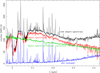 |
Fig. B.1. Typical spectrum without sky subtraction from a separate cube. The raw object spectrum (black), sky subtracted spectrum (red), sky spectrum (blue), and final telluric corrected science spectrum (green) are shown. The spectrum is from 3-18-2, an early-type star (showing the line of Brackett γ at 2.166 μm), which is a little brighter than the median magnitude of the full sample. |
To quantitatively test the impact of no dedicated sky exposure subtraction on the final spectra we now compare spectral properties of spectra with and without dedicated sky exposure subtraction. We therefore use only primary spectra, since they are more reliable. First we look at the overall properties as they come from the linear spectrum fit between 1.95 and 2.29 μm. We thus compare with the photometric properties. Firstly, we compare the zero point of the spectra with and without dedicated sky exposure subtraction. We find that in the mean and median it agrees very well with less than 0.005 mag difference. However, there is somewhat larger scatter without dedicated sky exposure subtraction by 12%–22%, depending on whether outliers are included or not. We also look at the other spectra obtained with the third spectrograph (those with an IFU number larger than 16) and found no increase, thus the larger scatter is likely caused by the missing dedicated sky exposure subtraction. Since the overall zeropoint is not necessarily important for relevant properties, we also look at other properties. Firstly, that is the spectral slope of the linear fit, which is well correlated with the H − K color. We fit for the two cases linearly. We find that the slope is consistent for with and without dedicated sky exposure subtraction. However, the intercept differs by 0.095 (equivalent of an H − K difference of 0.11). While that is significant, it is small compared to the single star error which is 0.36. The single star error is by 11% increased for stars with in-cube sky subtraction.
Next we look at the velocities. We find the velocities show no difference in the mean and scatter with and without dedicated sky exposure subtraction. Most stars are in systematic error regime, but the number of the stars above the systematic error regime is 13% higher without dedicated sky exposure subtraction than with subtraction (8%).
Now we look at the indices and derived properties from them. There are biases, which are often formally significant but always smaller than the scatter, at most 57% of the scatter. The bias of 0.06 is relatively large for H2O, but we know that it has a systematic error of at least 0.05. The next largest bias is for Brackett γ, which is also rather unimportant. For [Fe/H] the bias is 0.06 and for Teff, 120 K, resulting in larger values without sky subtraction. The scatter increases partly dedicated sky exposure without subtraction by up to 22% like for [Fe/H]. For Teff the scatter increases by 18%. Part of the differences with and without dedicated sky exposure subtraction are likely caused by spectrograph subsystem groups of IFUs and IFU effects.
There is some impact of applying only in-cube sky subtraction. However, this does not dominate the intrinsic variation. Since all fields have the missing arms, in-cube sky subtraction and any IFU dependent effect does not lead to differences between fields, and thus does not lead to any spurious discoveries in physical space. It is possible to construct a sample that is not affected by the suboptimal in-cube only sky subtraction by excluding the affected IFUs. The second part of the identification number corresponds to the IFU.
Appendix C: Tests of the velocities
In this appendix we test the quality of our radial velocity measurements made in Sect. 4.1. In particular, we test whether the absolute wavelength calibration is accurate and we compare our radial velocities to the APOGEE survey.
To test whether the absolute wavelength calibration of the spectra is good enough and that its error can be considered irrelevant, we used ATRAN atmospheric transmission spectra, which we smooth to the resolution of KMOS. We tested different ATRAN cases13, but found that the velocities vary at most by 2 km s−1 (in the case of the KMOS K-band model, which does not vary with the conditions in contrast with the other models), which is negligible compared to the other errors. To test for the velocity we cross-correlated the transmission spectra with the observed spectra before telluric correction of the primary targets. First, we cross-correlated the full spectra with the ATRAN models allowing offsets of up to |600| km s−1. In nearly all cases cross-correlation works. We find a median velocity of −3.5 km s−1 with a robust scatter of 4 km s−1. Since most of the telluric signal is at wavelengths very different from the spectral features, this might not be characteristic of the star velocities if the wavelength calibration error changes with wavelength. For most of our stars the velocity is based on late-type spectra between 2.18 μm and 2.425 μm. Therefore, we also cross-correlated our spectra with transmission spectra in that range and obtain an offset of −3.5 ± 4.5 km s−1. We also coadded spectra from the same exposure together and in that case the offset stays the same and the scatter reduces to about 1.5 km s−1, with no trend over time. Thus the error goes down with nearly  . This suggests that the scatter between different spectra in one exposure is probably caused by “noise”, like the spectral features in them. Because the CO band head in the spectra matters most for the velocity, we also cross-correlated around the strongest CO features, at the strongest atmospheric feature, which is at 2.317 μm. To cross-correlate only with it we used a range of 2.30 μm to 2.335 μm. For stars with CO lines this leads to bad results due to the many features there. Therefore we used only stars without CO, where the offset is −3 ± 5 km s−1. In conclusion, the spectra are wavelength calibrated well with no evidence of wavelength distortions. There is an offset of about 4 km s−1, which seems rather constant, with at most 5 km s−1 variation over the sample. We corrected for the calibration offset by adding 4 km s−1 to the raw velocities.
In addition we compared with external velocity measurements from the APOGEE survey (Majewski et al. 2017) in DR16 of SDSS (Ahumada et al. 2020). We find 20 common targets in the surveys, 19 stars with CO, and 1 foreground star with Brackett γ absorption. The velocities agree well in the mean (see Fig. C.1). However with original errors the scatter is larger than expected, as visible in the χ2 of 76. Since the agreement is better for stars with larger KMOS errors, we conclude that the KMOS errors are underestimated when the error is small. By requiring a χ2 of 19 we obtain that errors smaller than 4.2 km s−1 are underestimated. We therefore enlarge all errors below this limit to 4.2 km s−1. The reason for the error underestimation is not clear; it could be the limit of the algorithm or calibration uncertainty. In this sample we looked at stars with several exposures and find that their error is also underestimated. Since the exposures are obtained directly after each other with the same IFUs and only small dithers, this is not surprising, because this observing strategy leads to constant systematics in the instruments. After the error adjustment we find that the KMOS velocities are in the weighted average −1 ± 1 km s−1 smaller than the APOGEE velocities. Thus, our velocity scales are consistent. The enlargement of the errors does not impact our work, since the velocity differences between the survey stars are much larger than 4.2 km s−1.
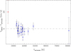 |
Fig. C.1. Velocity offset between KMOS and APOGEE. The star in red has no effective temperature in APOGEE; it shows cold stars features. The original KMOS errors are shown in color. The APOGEE errors are negligibly small in comparison. The errors after adjustment are shown in black. |
Appendix D: Metallicity calibration details
We show in Table D.1, the calibrator stars used for the derivation of our metallicity relation. Besides the names and metallicity from the literature, we also include the line indices measured by us and the derived metallicities.
Metallicity calibration stars.
Appendix E: Derived stellar properties
We present the properties for all successfully observed stars in Table E.1, available at the CDS. A successfully observed star is defined as having a measured line-of-sight velocity and/or at least S/N > 10. The table lists the following properties: Our identification number, coordinates, magnitudes in H, K, and when also available, in the J (all from Nishiyama et al. 2013) and IRAC bands (obtained from Churchwell et al. 2009; Spitzer Science Center 2009). If there is no good match or no detection, the magnitude value is set as −999.999. From our spectroscopy we present the overall S/N, the barycentric line-of-sight velocity and its error, the line indices of Brackett γ, Na I, Ca I, CO 2-0, H2O and their errors caused by S/N. For all stars with a CO based temperature, we also include the metallicity, its random error term and metallicity value when we omit KMOS/APOGEE or SINFONI/Thorsbro et al. (2020) for the calibration. For all stars we include the effective temperature with its random error. For stars without CO absorption (T > 6000 K), the temperature estimate is more uncertain as also visible in the error. For all stars we show an estimate of the intrinsic H − K color and of the extinction ordering parameter ext-order. We also provide the ripples flags. Values that could not be provided are set to −999.999.
Properties of secondary sources are often less reliable, in particular the photometric properties. The position is calculated from the brightest pixel offset relative to the primary source. That can be slightly offset when the maximum of either source is not within the IFU. The secondary sources are too faint and too confused for large-scale surveys, while the deeper GALACTICNUCLEUS survey does not cover the majority of our area. As such we do not provide J and IRAC magnitudes for our secondary sources. We estimate K and H magnitudes from the spectra by deriving the K-magnitude from the flux ratio, thereby comparing the secondary source relative to the primary source. Often this leads to underestimating its magnitude. We calculate the H magnitude by deriving a relationship between H − K color and K spectral slope between 1.95 μm and 2.29 μm for the primary sources. The scatter in this relationship is 0.37 mag. The spectral properties can be affected by flux from the primary source.
All Tables
All Figures
|
Fig. 1. Locations of the KMOS patrol fields of our survey. As shown by the colors, most were executed. Similar KMOS observations outside of this survey are also shown (Feldmeier-Krause et al. 2020, and in prep.). Together the full nuclear disk (Launhardt et al. 2002) is covered. The small black circle in the center shows the effective radius of the nuclear cluster (Gallego-Cano et al. 2020). The background shows a low-resolution extinction map in which the average extinction varies between AK = 0.45 and 2.93; see color bar. We made the extinction map from the catalog of Nishiyama et al. (2013). |
| In the text | |
|
Fig. 2. Observed CMDs of nuclear disk based on SIRIUS/2MASS (top, |l*| < 1.55° and |b*| < 0.3°) and inner bulge (bottom |l*| < 2° and 0.3° < |b*| < 1°. There are two sequences in the KMOS bulge data because of the variable extinction (see also Nogueras-Lara et al. 2018a). In blue we show all stars within the KMOS fields. The KMOS and APOGEE target stars are shown in black and red, respectively. The shown isochrones are from PARSEC. The gray polygons outline our CMD selection of targets. The blue H − K color limit varies slightly from field to field. |
| In the text | |
|
Fig. 3. Number of targets per square arcminute in a KMOS OB as a function of radial distance in arcminutes from the field center. The overall target numbers are divided by 24 to show the typical target density per KMOS field. Fields 1 and 5 are the most extreme fields in terms of target density: field 1 is at the higher density limit and field 5 is at the lower density limit and also has fewer observed stars because one subset was not successfully observed. The downward-facing arrows mark bins in which no star was observed. |
| In the text | |
|
Fig. 4. Barycentric velocities of all stars with measurements as a function of Galactic longitude. |
| In the text | |
|
Fig. 5. Na (top) and Ca (bottom) as a function of CO index. For Na all stars with an S/N > 20 are shown; the value where the intrinsic scatter of CO and Na is of the size of the measurement error. For Ca the S/N is lower and thus only stars with an S/N > 40 are plotted. |
| In the text | |
|
Fig. 6. CO and Brackett γ equivalent widths for all stars. Stars with early-type lines are confirmed with visual inspection of the spectra. In the top panel the stars with an S/N < 20 are shown; in the bottom panel the stars with an S/N > 20 are shown. This S/N is the approximately border of the nearly complete regime of spectral classification. The lines divide absorption (negative) and emission. |
| In the text | |
|
Fig. 7. Index windows together with a typical spectrum. The continuum windows are shown hatched, the feature windows cross hatched. The spectrum is typical for a primary target spectrum in S/N and CO and Na index values. In the top panel the molecular indices are shown; in the bottom panel the atomic indices are shown. |
| In the text | |
|
Fig. 8. H2O index as a function of extinction corrected magnitude K0 for stars with S/N > 20. Unusual sources are indicated with open symbols, blue circles (early-type or young stellar objects), or boxes (AGB with Brackett γ). Sources with H2O index below 0.7 are probably AGB stars. |
| In the text | |
|
Fig. 9. Metallicity derivation. Top: calibration of metallicity based on CO and Na EW. The large symbols represent the 183 used calibration spectra; the symbol shape shows the source of spectra and metallicity (Magrini et al. 2010; Thorsbro et al. 2020; Ahumada et al. 2020; Arentsen et al. 2019). The value is indicated by the color within SINF indicates SINFONI. The background shows the derived relation; the color range saturates below [Fe/H] < −2.5 and above [Fe/H] > 0.6 (the range of the calibrators.), where the derived values are based on more uncertain extrapolation. The two vertical lines separate the application of the high and low CO solutions; in the overlap region in between both high and low CO solutions are used to derive metallicities. The small dots show all our KMOS targets with S/N > 30 and a CO based velocity. The background shows the derived value only for areas where either calibrators or the nuclear stars have coverage. Bottom: comparison between literature (x-axis) and our metallicities (y-axis). The thick black line indicates the identity line; the thin lines bracket the typical uncertainty. Stars are coded by CO depth; the hottest have the smallest depth. |
| In the text | |
|
Fig. 10. Metallicity distribution of survey stars. All 2734 stars with CO absorption and S/N > 30 are shown. At the top, the median statistical error of stars passing these cuts are indicated in black and in blue the calibration uncertainty, which does not depend on metallicity. |
| In the text | |
|
Fig. 11. Temperature calibration for stars with CO absorption. For CO EW larger than −21.5 Å, the equations of Mármol-Queraltó et al. (2008) are used. These equations use our [Fe/H] determination. Below −22.5 the calibration by Feldmeier-Krause et al. (2017), corrected for the offset between the two, is used. Between these values (indicated by the two black lines) there is a linear transition between the two relations. The diagonal strip shows the uncorrected relation by Feldmeier-Krause et al. (2017). It is plotted for |[Fe/H]| < 0.075. The color scales saturate outside of 2600 K and 5800 K. The dots show our KMOS targets with S/N > 30. |
| In the text | |
|
Fig. 12. Temperature distribution of survey stars. The spectral class (borders) are indicated in the top of the plots. Top panel: all stars with S/N > 20, that is, all stars that were classifiable (with a single exception). The latter is grouped together with the young stellar objects at 8000 K. This temperature and that of the hotter stars is qualitative based on spectral feature existence. Bottom panel: zoom-in of the colder stars (stars with CO absorption) with S/N > 30, for which temperatures from line indices are calculated. |
| In the text | |
|
Fig. B.1. Typical spectrum without sky subtraction from a separate cube. The raw object spectrum (black), sky subtracted spectrum (red), sky spectrum (blue), and final telluric corrected science spectrum (green) are shown. The spectrum is from 3-18-2, an early-type star (showing the line of Brackett γ at 2.166 μm), which is a little brighter than the median magnitude of the full sample. |
| In the text | |
|
Fig. C.1. Velocity offset between KMOS and APOGEE. The star in red has no effective temperature in APOGEE; it shows cold stars features. The original KMOS errors are shown in color. The APOGEE errors are negligibly small in comparison. The errors after adjustment are shown in black. |
| In the text | |
Current usage metrics show cumulative count of Article Views (full-text article views including HTML views, PDF and ePub downloads, according to the available data) and Abstracts Views on Vision4Press platform.
Data correspond to usage on the plateform after 2015. The current usage metrics is available 48-96 hours after online publication and is updated daily on week days.
Initial download of the metrics may take a while.