| Issue |
A&A
Volume 647, March 2021
|
|
|---|---|---|
| Article Number | A81 | |
| Number of page(s) | 13 | |
| Section | The Sun and the Heliosphere | |
| DOI | https://doi.org/10.1051/0004-6361/202039491 | |
| Published online | 12 March 2021 | |
Excitation and evolution of coronal oscillations in self-consistent 3D radiative MHD simulations of the solar atmosphere⋆
1
Rosseland Centre for Solar Physics, University of Oslo, PO Box 1029, Blindern 0315, Oslo, Norway
e-mail: petra.kohutova@astro.uio.no
2
Institute of Theoretical Astrophysics, University of Oslo, PO Box 1029, Blindern 0315, Oslo, Norway
Received:
22
September
2020
Accepted:
15
January
2021
Context. Solar coronal loops are commonly subject to oscillations. Observations of coronal oscillations are used to infer physical properties of the coronal plasma using coronal seismology.
Aims. Excitation and evolution of oscillations in coronal loops is typically studied using highly idealised models of magnetic flux tubes. In order to improve our understanding of coronal oscillations, it is necessary to consider the effect of realistic magnetic field topology and evolution.
Methods. We study excitation and evolution of coronal oscillations in three-dimensional (3D) self-consistent simulations of solar atmosphere spanning from the convection zone to the solar corona using the radiation-magnetohydrodynamic (MHD) code Bifrost. We use forward-modelled extreme-ultraviolet emission and 3D tracing of magnetic field to analyse the oscillatory behaviour of individual magnetic loops. We further analyse the evolution of individual plasma velocity components along the loops using wavelet power spectra to capture changes in the oscillation periods.
Results. Various types of oscillations commonly observed in the corona are present in the simulation. We detect standing oscillations in both transverse and longitudinal velocity components, including higher-order oscillation harmonics. We also show that self-consistent simulations reproduce the existence of two distinct regimes of transverse coronal oscillations: rapidly decaying oscillations triggered by impulsive events and sustained small-scale oscillations showing no observable damping. No harmonic drivers are detected at the footpoints of oscillating loops.
Conclusions. Coronal loop oscillations are abundant in self-consistent 3D MHD simulations of the solar atmosphere. The dynamic evolution and variability of individual magnetic loops suggest that we need to re-evaluate our models of monolithic and static coronal loops with constant lengths in favour of more realistic models.
Key words: magnetohydrodynamics (MHD) / Sun: corona / Sun: magnetic fields / Sun: oscillations
Movies associated to Figs. 2, 4, and 10 are available at https://www.aanda.org
© ESO 2021
1. Introduction
Coronal loops, the basic building blocks of the solar corona, are commonly subject to oscillatory behaviour. Because of their magnetic structure, they act as wave guides and can support a variety of wave modes (see e.g., reviews by Nakariakov & Verwichte 2005; Nakariakov & Kolotkov 2020). Various types of wave modes have been reported at coronal heights; these include nearly incompressible transverse oscillations in the direction perpendicular to the loop axis (Aschwanden et al. 1999; Nakariakov et al. 1999; Verwichte et al. 2013), compressible longitudinal oscillations along the loop axis (Berghmans & Clette 1999; De Moortel et al. 2000), and incompressible torsional oscillations (Kohutova et al. 2020b). Transverse oscillations of coronal loops are by far the most commonly observed type. They were first discovered in the TRACE observations of coronal loops following a solar flare (Aschwanden et al. 1999; Nakariakov et al. 1999) and since then have been studied extensively through high-resolution solar observations, numerical simulations, and analytical theory. The most commonly reported oscillation periods lie in the range of 1−10 min, and the oscillation amplitudes range from a few hundred to several thousand kilometres. Most of the observed transverse coronal loop oscillations have been identified as corresponding to either standing or propagating kink modes. This mode identification is based on modelling individual coronal loops as cylindrical flux tubes (Edwin & Roberts 1983). It should however be noted that the density structuring in the corona is more complex than this and assumptions about the individual mode properties based on idealised modelling of homogeneous plasma structures do not always apply in the non-homogeneous and dynamic environment of the real solar corona (e.g., Goossens et al. 2019). The fundamental harmonic of the standing kink mode is the most commonly observed, where the footpoints of the coronal loop act as nodes and the point of maximum displacement amplitude lies at the loop apex. Despite the fundamental harmonic being the most intuitive resonant response of a line-tied magnetic field line to an external perturbation, excitation of higher order harmonics is also perfectly viable; higher order harmonics have also been identified in coronal loop oscillations (Verwichte et al. 2004; Duckenfield et al. 2018).
Transverse oscillations of coronal loops are commonly used for coronal seismology (see e.g., reviews by De Moortel 2005; De Moortel & Nakariakov 2012; Nakariakov & Kolotkov 2020). Coronal seismology is a powerful method that relies on using oscillation parameters that are readily observable in the coronal imaging and spectral data to deduce plasma properties such as density, temperature, magnetic field strength or density structuring, which are otherwise very challenging to measure directly. The accuracy of the seismologically deduced quantities is however limited by somewhat simplifying assumptions of modelling coronal structures as homogeneous plasma cylinders and is subject to uncertainties caused by projection and line-of-sight effects.
Transverse coronal loop oscillations are often classified as occurring in two regimes: large-amplitude rapidly damped oscillations and small-amplitude seemingly ‘decayless’ oscillations. Large-amplitude oscillations are typically triggered by an external impulsive event, which is usually easy to identify, such as a blast wave following a solar flare (e.g., White & Verwichte 2012). Amplitudes are of the order of 1 Mm and the oscillations are rapidly damped within 3−4 oscillation periods.
Small-amplitude oscillations are observed without any clearly associated driver and can persist for several hours (Wang et al. 2012; Nisticò et al. 2013; Anfinogentov et al. 2015). Their amplitudes are of the order of 100 km and they show no observable damping. Even though it is clear they must be driven by some small-scale abundant process, the exact excitation mechanism of this oscillation regime is unclear. Several excitation mechanisms have been proposed to explain the persistent nature of these oscillations. These include mechanisms acting at coronal heights such as the onset of thermal instability in the corona (Kohutova & Verwichte 2017; Verwichte & Kohutova 2017), the presence of siphon flows in the coronal loop (Kohutova & Verwichte 2018), self-oscillation of coronal loops due to interaction with quasi-steady flows (Nakariakov et al. 2016; Karampelas & Van Doorsselaere 2020), and footpoint-concentrated drivers. A commonly assumed excitation mechanism is associated with turbulent vortex flows which are ubiquitous in the lower solar atmosphere (Carlsson et al. 2010; Shelyag et al. 2011; Liu et al. 2019) and result in random footpoint buffeting. This is typically modelled as a stochastic driver at the footpoints (e.g., Pagano & De Moortel 2019). Such a driver however does not reproduce the observational characteristics of this type of oscillation, in particular the stability of the oscillation phase and lack of any observable damping (Nakariakov et al. 2016). It has been proposed that a footpoint driver of the form of a broadband noise with a power-law fall-off can in principle lead to excitation of eigenmodes along coronal loops (Afanasyev et al. 2020), but this has not been tested through MHD simulations. Finally, excitation of transverse oscillations through solar p-mode coupling has also been proposed in several studies (Tomczyk & McIntosh 2009; Morton et al. 2016, 2019; Riedl et al. 2019). As p-modes correspond to acoustic waves generated by turbulent flows in the solar convection zone, they are subject to acoustic cut-off at the β = 1 equipartition layer. High magnetic field inclinations can however lead to p-mode leakage into chromosphere even for frequencies below the cut-off frequency (De Pontieu et al. 2004), and to subsequent coupling to different magnetoacoustic wave modes (Santamaria et al. 2015). However, three-dimensional (3D) MHD simulations of coronal fluxtubes with a gravity-acoustic wave driver at the footpoints did not reveal any evidence of the acoustic driving leading to significant transverse displacement of the fluxtubes at coronal heights (Riedl et al. 2019).
It is in reality very likely that the oscillatory behaviour observed in the corona is caused by a combination of several different excitation mechanisms. Three-dimensional MHD simulations of the solar atmosphere spanning from the convection zone to the corona in principle include all of the potential mechanisms discussed above. However, so far only impulsively generated rapidly damped coronal loop oscillations have been studied in such 3D MHD simulations (Chen & Peter 2015), which show a good match between damping rates and observed impulsively generated oscillations. Such numerical works also highlight the implications of observational limitations for coronal seismology, as they enable direct comparison of seismologically deduced and real values of physical quantities. Detailed properties of transverse coronal loop oscillations have been studied numerically in great detail in recent years, including their evolution, damping and development of instabilities and resulting non-linear dynamics (e.g., Antolin et al. 2014; Magyar & Van Doorsselaere 2016; Karampelas et al. 2017). However, most of these studies employ simplified geometries that model coronal structures as straight uniform flux tubes. Additionally, such studies also rely on artificially imposed harmonic footpoint drivers (Karampelas et al. 2017; Pagano & De Moortel 2017), without discussing where these drivers originate. Such an approach makes it possible to isolate individual effects of interest, and focus on evolution at small scales through techniques such as adaptive mesh refinement (e.g., Magyar et al. 2015) due to obvious computational limitations that come with studying physical mechanisms operating at vastly different spatial scales. There is nevertheless a need for a more complex approach to see how such effects manifest in a realistic solar atmosphere setup and to identify their observational signatures.
In this work we investigate the presence of oscillations of coronal loops in a simulation spanning from the convection zone to the corona, with a realistic dynamics of the lower solar atmosphere, geometry of the magnetic field and density structuring. Furthermore, this is the first time that the excitation of transverse coronal oscillations has been analysed in a self-consistent simulation of the solar atmosphere. We use a combination of forward modelling of coronal extreme-ultraviolet (EUV) emission and evolution of physical quantities along magnetic field to determine oscillation characteristics.
2. Numerical model
We analyse coronal oscillations in the numerical simulation of magnetic enhanced network spanning from the upper convection zone to the corona (Carlsson et al. 2016) using 3D radiation MHD code Bifrost (Gudiksen et al. 2011). This simulation was previously used to analyse the oscillatory behaviour of chromospheric fibrils by Leenaarts & Carlsson (2015) and to study signatures of propagating shock waves by Eklund et al. (2021).
Bifrost solves resistive MHD equations and includes non-local thermodynamic equilibrium (LTE) radiative transfer in the photosphere and low chromosphere, and parametrised radiative losses and heating in the upper chromosphere, transition region and corona. The simulation includes the effects of thermal conduction parallel to the magnetic field and the non-equilibrium ionisation of hydrogen.
The physical size of the simulation box is 24 × 24 × 16.8 Mm. The vertical extent of the grid spans from 2.4 Mm below the photosphere to 14.4 Mm above the photosphere, which corresponds to z = 0 surface and is defined as the (approximate) height where the optical depth τ500 is equal to unity. The simulation is carried out on a 504 × 504 × 496 grid. The grid is uniform in the x and y direction with grid spacing of 48 km. The grid spacing in the z direction is non-uniform in order to resolve steep gradients in density and temperature in the lower solar atmosphere and varies from 19 km to 98 km. The domain boundaries are periodic in the x and y directions and open in the z direction. The top boundary uses characteristic boundary conditions such that any disturbances are transmitted through the boundary with minimal reflection. Tests of the characteristic boundaries implemented in Bifrost suggest that the reflection of the energy from the upper boundary is 5% or less (Gudiksen et al. 2011). At the bottom boundary the flows are let through and the magnetic field is passively advected while keeping the magnetic flux through the bottom boundary constant. The average horizontal pressure is driven towards a constant value with a characteristic timescale of 100 s. This pressure node at the bottom boundary gives rise to acoustic wave reflection which resembles the refraction of waves in the deeper solar atmosphere. This leads to global radial box oscillations with a period of 450 s, which are a simulation counterpart of solar p-modes (Stein & Nordlund 2001; Carlsson et al. 2016); radial modes in this context correspond to oscillations in horizontally averaged quantities polarised along the z-axis in a cartesian simulation box.
The photospheric magnetic field has an average unsigned value of about 50 G and is concentrated in two patches of opposite polarity separated by about 8 Mm; this leads to the development of several magnetic loops at coronal heights (Fig. 1). Upon initialisation of the simulation, the large-scale magnetic field configuration was determined by potential extrapolation of the vertical magnetic field specified at the bottom boundary. After inserting the magnetic field into the domain, it is quickly swept around by convective motions. These lead to magnetic field braiding and associated Ohmic and viscous heating which together maintain high temperature in the chromosphere and corona (see e.g., Carlsson et al. 2016; Kohutova et al. 2020a for further details of the numerical setup).
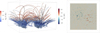 |
Fig. 1. Left: magnetic configuration of the simulation showing the temperature profile of the individual field lines. The simulation domain has physical size of 24 × 24 × 16.8 Mm. The simulation snapshot shown corresponds to t = 180 s after the non-equilibrium ionisation of hydrogen has been switched on. Right: line-of-sight component Bz of the photospheric magnetic field at t = 180 s. |
3. Transverse oscillations observable in forward-modelled EUV emission
In order to compare the oscillatory behaviour seen in the numerical simulation with the commonly observed transverse coronal loop oscillations seen by the Atmospheric Imaging Assembly on board the Solar Dynamics Observatory (SDO/AIA), we forward model the EUV emission using the FoMo code (Van Doorsselaere et al. 2016). The FoMo code is capable of modelling optically thin coronal emission in individual spectral lines as well as in the broadband SDO/AIA channels. The instrumental response function of a given SDO/AIA bandpass κα is calculated for a grid of electron densities ne and temperatures T as
where G(λα, ne, T) is the contribution function calculated from the CHIANTI database, Rα(λα) is the wavelength-dependent response function of the given bandpass, and the wavelength integration is done over all spectral lines within the given bandpass. κα is then integrated along the line-of-sight parallel to the z-axis, which corresponds to looking straight down on the solar surface.
Figure 2 shows forward modelled emission in the SDO/AIA 171 Å bandpass, which is dominated by the Fe IX line with a formation temperature of log T = 5.9. In order to highlight the oscillatory motion, a time–distance plot is created by taking the intensities along a slit across the loop structures and stacking them in time. Several oscillating structures can be seen in this plot, suggesting transverse coronal loop oscillations are abundant in the model. The forward-modelled EUV emission in the model is more diffuse (Fig. 3) and subject to less observable structuring across the magnetic field than coronal emission typically observed at similar wavelengths, where the individual coronal loops can appear very threadlike (e.g., Peter et al. 2013; Williams et al. 2020). We note that the simulation does not include magnetic flux emergence which means the loops are not mass loaded and pushed into the corona from the lower solar atmosphere. Instead, the dense loops are filled via chromospheric evaporation caused by localised heating (Kohutova et al. 2020a). However, some transverse structuring is still present thanks to the temperature variation across different magnetic field lines. This makes it possible to see the oscillatory behaviour of the individual coronal strands in the intensity time–distance plot.
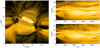 |
Fig. 2. Left: forward-modelled emission in the SDO/AIA 171 Å channel at t = 180 s. Dashed lines outline projected positions of the studied field lines F1−F5. Right: time–distance plots showing temporal evolution along the slits shown in blue. The vertical axis corresponds to the distance along the slit. Several oscillating structures are visible in the time–distance plots. The dashed contour in plot A outlines a propagating disturbance. An animation of this figure is available online. |
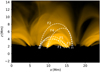 |
Fig. 3. Forward-modelled emission in the SDO/AIA 171 Å channel at t = 180 s viewed along the y-axis. Dashed lines outline the projected positions of the studied field lines F1−F5. |
4. Transverse oscillations of individual field lines
Coronal loops in our study are represented by closed magnetic field lines extending into the corona. Several of these have enhanced densities compared to the surroundings. Density-enhanced coronal loops with well-defined boundaries in the simulation are however less common than what is usually observed in the corona. As there is no flux emergence mechanism included in the simulation, most of the dense loops are filled by chromospheric evaporation instead of being lifted up from the lower atmosphere.
The magnetic field in the simulation domain is constantly evolving and undergoing complex motions which include sideways displacement, oscillatory motion, and torsional and upward/downward motion resulting in the change of the total coronal loop length. Therefore, in order to investigate the oscillatory behaviour of coronal loops in the simulation, it is necessary to trace the evolution of the corresponding magnetic field lines through both time and space. To do this, we use a field-tracing method previously used by Leenaarts & Carlsson (2015) and Kohutova et al. (2020a). A magnetic field line is defined as a curve in 3D space r(s) parametrised by the arc length along the curve s, for which dr/ds = B/|B|.
The tracing of the evolution of magnetic field lines is done by inserting seed points (one seedpoint per tracked field line) into the locations in the simulation domain which show oscillatory behaviour in the velocity time–distance plots. This is equivalent to tracking the evolution of magnetic connectivity of an oscillating plasma element. The seed points are then passively advected forward and backward in time using the velocity at the seed point position. At every time-step the magnetic field is then traced through the instantaneous seed point position in order to determine the spatial coordinates of the traced field line. This is done using the Runge–Kutta–Fehlberg integrator with an adaptive step size. Even though the accuracy of this method is limited by the size of the time-step between the two successive snapshots (i.e. 10 s), it works reasonably well provided that the magnetic field evolution is smooth and there are no large-amplitude velocity variations occurring on timescales shorter than the size of the time-step. We note that this method leads to a jump in the field-line evolution in the instances where magnetic reconnection occurs.
We investigate the evolution of five different fieldlines labelled F1 to F5 (Fig. 4). We note that the footpoints of the chosen magnetic loops lie in regions of enhanced vorticity. We analyse the evolution of the temperature, density, and three velocity components, vL, vV and vT along each loop. The longitudinal velocity vL = v ⋅ T corresponds to the velocity component aligned with the tangent vector of the magnetic fieldline given by T = B/|B|. The vertical velocity vV = v ⋅ N is the velocity component along the normal vector of the field line given by 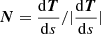 and corresponds to the motion in the plane of the coronal loop. Finally the transverse velocity component along the binormal vector is given by vT = v ⋅ R where R = T × N and corresponds to transverse motion perpendicular to the plane of the coronal loop. Unit vectors T, N, and R together form an orthogonal coordinate system equivalent to a Frenet frame of reference. Such a coordinate frame is well suited to analysing oscillations in complex 3D magnetic field geometries and is commonly used in such studies (e.g., Felipe 2012; Leenaarts & Carlsson 2015; González-Morales et al. 2019). We further calculate a wavelet power spectrum (Torrence & Compo 1998) for all three velocity components at three different locations along the field line; close to the loop footpoints 1 Mm above the transition region (the height of which is tracked with time) at the beginning and end of the fieldline (labelled FP1 and FP2 for left and right footpoints respectively) and at the loop apex halfway between FP1 and FP2.
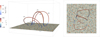 |
Fig. 4. Left: location of field lines F1−F5 chosen for analysis of oscillatory behaviour shown at t = 1500 s. We also show the z-component of vorticity ωz at z = 0, i.e. in the photosphere. The footpoints of analysed field lines are embedded in the intergranular lanes with strong vortex flows. Right: configuration viewed from above. An animation of this figure is available online. |
4.1. Field line F1
Field line F1 is a short, closed field line in the centre of the domain. For most of its lifetime it is not subject to any major changes, however at t = 2100 s it rapidly contracts and finally disappears in the chromosphere. The evolution of the physical quantities along the field line is shown in Fig. 5. The field line is subject to strong base heating starting at t ∼ 600 s resulting in evaporative upflows of the chromospheric plasma into the loop, observable in the vL component for about 200 s. We identify this as a consequence of a global disturbance propagating from the centre of the domain outwards, visible in Fig. 2, which likely triggers reconnection in the affected loops, leading to increased Joule and viscous heating. This is accompanied by an onset of the oscillatory behaviour lasting from t = 600 s to t = 1100 s. The oscillation is most clearly seen in the vV component of the velocity (marked as segment b in Fig. 5) which corresponds to vertical polarisation (i.e. polarisation in the plane of the loop). In total, three oscillation periods are observable, with the oscillation period being around 200 s. The lack of periodic displacement at the loop footpoints as compared with the periodic evolution at the loop apex lacking phase shift indicate that the oscillation is standing, and not driven by footpoint motions. This is accompanied by an oscillation with matching period in vL velocity component, that is along the magnetic field, with the oscillation profile matching the second harmonic of a standing longitudinal mode (segment a in Fig. 5). The wavelet analysis also reveals the presence of an oscillation with a period of 250 s in the vV with later onset having similar characteristics and lasting from t = 1300 s to t = 2100 s, that is until the impulsive event that leads to rapid contraction of the loop. This oscillation is marked as segment c in the vV evolution plot. Some attenuation of the oscillation is observable, especially in the initial stages. We attribute the increase of the standing oscillation period to the increase in density of the coronal loop plasma. Finally, a large-amplitude disturbance (∼10 km s−1 amplitude at the apex) can be observed in the evolution of the transverse velocity component vT from t = 1200 s to t = 1600 s. However, as only one oscillation period is observable, we refrain from drawing any conclusions about the oscillation characteristics.
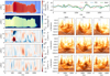 |
Fig. 5. Left: evolution of temperature, density and three velocity components vL, vT and vV along the field line F1. The x axis corresponds to time and the y axis corresponds to the position along the field line. Vertical dotted lines mark segments with oscillatory behaviour. Top right: evolution of the transverse component of the velocity vT at the footpoints FP1 and FP2 (red and blue respectively) 1 Mm above the transition region and at the fieldline apex halfway between the two footpoints (green). Bottom right: wavelet spectra for the three velocity components taken at the apex of the field line and at the footpoints FP1 and FP2. Dark colour corresponds to high power. The hatched region corresponds to the area outside of the cone of influence. White lines correspond to 95% significance contours. |
4.2. Field line F2
Field line F2 has a length of over 20 Mm (Fig. 6). During the initial 400 s of its evolution, there is a clear accumulation of cool and dense material in the coronal part of the loop, most likely through the condensation of coronal plasma. Condensation phenomena in this simulation have been studied in detail by Kohutova et al. (2020a). The loop evolution is dynamic and affected by impulsive events occurring at coronal heights. At t ∼ 500 s a discontinuity in temperature and velocity evolution is visible similar to what is observed in F1. An associated temperature increase and jump in field line tracking suggest this corresponds to a reconnection event. We note that the discontinuity in the F1 evolution is observable with a slight delay compared to F2, suggesting it is caused by a large-scale disturbance propagating across the domain. The evolution of the transverse velocity component vT shows several large-amplitude disturbances at the apex of the loop with typical amplitudes of 20 km s−1; these are not mirrored by the velocity at the footpoints and therefore not driven by footpoint motions. The lack of any associated large-amplitude deviations in the plasma density and temperature suggests that these deviations are caused by external disturbances, that is not originating in the loop. The field line F2 shows clear oscillation in the longitudinal velocity component vL with a period of ∼250 s (marked as segment a in Fig. 6). These periodic disturbances are propagating from the footpoint FP2 to footpoint FP1 at a speed of ∼90 km s−1, which is close to the average local sound speed (we note that there are also some signatures of propagation in opposite direction). The longitudinal oscillation is visible in both the field-line evolution plot and the wavelet spectra and lasts for most of the duration of the simulation sequence until t = 2000 s. The wavelet spectrum shows a slight gradual decrease in period, probably linked to the decrease in the total loop length. No clear attenuation is observable for the duration of the oscillation. The loop is also subject to shorter period transverse oscillations visible in the vT velocity component with periods of 180 s (segment c), and a similar oscillation can also be seen in the vV evolution (segment d). The oscillation in vT follows a large initial displacement that occurred at t = 900 s and is rapidly attenuated in a similar manner to the large-amplitude damped oscillations excited by impulsive events observed in the solar corona. In total, four oscillation periods can be observed before the oscillation completely decays. Finally, we also note that high-frequency transverse oscillations can be observed in the loop during the initial 400 s with period less than 100 s (segment b). The period changes during the oscillation duration, likely because of the change in the conditions in the loop linked to the condensation formation discussed earlier. In total, five oscillation periods are observable with no clear damping.
4.3. Field line F3
Field line F3 undergoes rapid expansion during the impulsive event at occurring at t = 500 s discussed above, during which the total length of the loop doubles (Fig. 7). This disturbance is also very clear in the evolution of the velocity component vT at both footpoints and the loop apex and manifests itself as a transverse displacement with the velocity amplitude of 47 km s−1 at the apex. An oscillation is visible in the transverse velocity component vT (segment b in Fig. 7) observable during the entire duration of the simulation with periodicity of ∼180 s, which changes slightly over time. This oscillation is also picked up in the evolution of the vV component (segment c), because of the nature of our coordinate system and the fact that transverse coronal loop oscillations can have any polarisation in the plane perpendicular to the magnetic field vector. There is no observable damping even following the impulsive event, and the amplitude of the transverse oscillation remains around 5 km s−1 throughout the duration of the simulation. The transverse oscillation is clearly present even before the impulsive event, suggesting that the impulsive event does not act as the primary driver of the oscillation. No persistent phase shift in a single direction is observable between the vT evolution at the loop apex and the two footpoints. The position of maximum vT amplitude varies between s = 5 Mm and s = 10 Mm along the loop. This suggests that the oscillation corresponds to a standing transverse oscillation, as the velocity amplitude is greater at the loop apex than it is at close to the loop footpoints and there is no indication that the oscillation is driven by the footpoint motion. The observed oscillation mode likely corresponds to the fundamental harmonic, as only one oscillation antinode is observed. We note that despite the oscillatory behaviour being obvious from the plots of vT and vV evolution, it is not picked up by wavelet spectra above 95% confidence level. Oscillations with a similar period are present in the evolution of the vL velocity component (segment a). Oscillatory behaviour of F3 is also observable in the time–distance plot using synthetic SDO/AIA 171 Å observations shown in Fig. 2. The position of the loop F3 in the time–distance plot starts at yt = 5 Mm along the slit and, following the expansion, gradually moves outwards and away from the centre of the domain towards yt = 2.5 Mm. From the forward-modelled intensity it is also clear that several loops in the vicinity of F3 are also subject to oscillations with similar period and duration to the F3 oscillation. These field lines are therefore likely part of a larger loop bundle that is subject to a collective transverse oscillation.
4.4. Field line F4
Field line F4 initially corresponds to a short coronal loop with an initial length of 10 Mm (Fig. 8). During the first 400 s the loop expands, nearly doubling its length. Another dramatic expansion of the loop starts after t = 1500 s, after which the loop apex eventually reaches the upper boundary and the loop becomes an open field line at t = 1670 s. An oscillation is observable in the longitudinal component of velocity vL between t = 350 s and t = 850 s (segment a in Fig. 8). The oscillation profile has a node close to the apex of the loop, reminiscent of a second longitudinal harmonic. The period of the longitudinal oscillation is ∼200 s, and increases over time. No clear periodic behaviour is visible in the evolution of vT and vV velocity components during the lifetime of the closed field line. After the field line opens, the total length integrated along the field line jumps to approximately half of its original value. Quasi-periodic disturbances propagating from the upper boundary downwards can be observed in the evolution of vL. These appear coupled to high-frequency oscillatory behaviour with a ∼60 s period observable in vT and vV components for the remainder of the lifetime of the open field line. As these are likely to be an artifact from the open boundary, we do not analyse them further. We also note that large-amplitude transverse oscillation pattern is observable in the synthetic EUV emission close to the projected position of F4. As this does not seem to match with the evolution of the transverse velocity vT of F4, we conclude that most of the emission comes from the lower lying loops. Again, several strands in this region can be seen to oscillate in phase, pointing to a collective transverse oscillation.
4.5. Field line F5
The evolution of field line F5 is shown in Fig. 9. This field line approaches F2 at t = 1500 s (Fig. 4), but for most of the duration of the simulation, the two loops evolve independently from each other without signs of collective behaviour. Similarly to field lines discussed above, F5 is also affected by the impulsive event at t = 500 s that sweeps across the coronal loops in the centre of the simulation domain (Fig. 2). Oscillatory behaviour in the longitudinal velocity component vL with the spatial structure reminiscent of a second harmonic is identifiable from t = 500 s to approximately t = 1250 s (segment a in Fig. 9), after which the periodic evolution becomes less clear and harder to identify. The oscillation node lies slightly off-centre closer to FP1; this oscillatory behaviour is therefore also picked up in the wavelet spectrum for the evolution of vL at the apex, although with evolving period. The wavelet spectra further show a strong signal for the periodicity in the vertical component of the velocity vV. Vertical oscillations with ∼250 s period are also clear in the field-line evolution plot (segment c). Oscillation with similar characteristics is also visible in the vT component (segment b), although less clearly. Both vT and vV oscillations have points of maximum amplitude located in the upper parts of the loop, suggesting the oscillation is not driven by transverse displacement of the footpoints. This is further supported by the line plot of the evolution of the transverse velocity component, which shows that the velocity amplitude at the apex always dominates over velocity amplitude at the loop footpoints. We note that the evolution of the loop length is coupled to the oscillatory behaviour, as clearly visible from the evolution of the position of the footpoint FP2 in the loop evolution plot. This suggests that the loop is undergoing a standing oscillation with with a period of ∼250 s polarised in the vertical direction. Unlike horizontally polarised standing oscillations, these affect the total length of the loop and lead to periodic inflows and outflows from the loop centre as the loop expands and contracts. The oscillation cannot be indisputably linked to a single impulsive event, but it follows two successive temperature increases in the loop plasma occurring at t = 300 s and t = 600 s respectively.
4.6. Footpoint evolution
We further calculate Fourier power spectra for each cell in the horizontal plane of the simulation box at two heights: at z = 1.4 Mm in the chromosphere and at z = 10 Mm in the corona. We sum the power for all frequencies between 1.67 mHz and 16.7 mHz, corresponding to periods of 600 s and 60 s respectively, which covers the range of periods of oscillatory behaviour detected in the simulation. The resulting integrated power maps therefore highlight locations with increased oscillatory power regardless of the period of the oscillation; we compare these with the instantaneous positions of magnetic loop footpoints (Fig. 10).
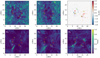 |
Fig. 10. Top: integrated power between 1.67 mHz and 16.7 mHz for vx (left), vy (centre) components of the velocity at z = 1.4 Mm in the chromophere and line-of-sight photospheric magnetic field at t = 180 s (right). Bottom: integrated power between 1.67 mHz and 16.7 mHz for vx (left), vy (centre) and vz (right) components of the velocity at z = 10 Mm in the corona. Coloured circles with 1 Mm diameter are centred on positions of footpoint coordinates at z = 1.4 Mm at t = 0 s and colour-coded as follows: F1-black, F2-red, F3-purple, F4-green, and F5-orange. An animation of this figure for the full duration of the simulation is available online. |
This evolution highlights the dynamic nature of coronal loops, as their footpoints are not static but evolve throughout the entire simulation as they get dragged around by convective flows. Such changes occur on the same timescales as the evolution of the line-of-sight component of the photospheric magnetic field. Occasionally, the evolution is more rapid, most likely when involving impulsive reconnection events at coronal heights. In general, footpoints of oscillating loops are not embedded in locations with increased oscillatory power. A harmonic driver is therefore not a prerequisite for onset of coronal loop oscillations.
5. Discussion
An important point for consideration is the applicability of the field-line-tracing method that is used to study the field-line evolution in the instances of magnetic reconnection. Tracing of the magnetic field lines is equivalent to tracing the grid points in the simulation domain which are magnetically connected. In the corona the matter and energy transport happens along the magnetic field, tracing the magnetic field lines is therefore the closest we can get to studying the true evolution of coronal structures without being affected by line-of-sight effects, which can significantly influence determination of oscillation parameters (see e.g., De Moortel & Pascoe 2012). When a magnetic loop ‘reconnects’, the magnetic connectivity of a certain part of the loop changes. However, advecting the seed points initially placed into regions where oscillations were detected ensures we keep tracing the magnetic connectivity of the oscillating part even if reconnection occurs in other parts of the loop. We therefore argue that this approach remains the most feasible way of tracing the true evolution of coronal structures.
We note that evolution in line-of-sight-integrated emission does not necessarily copy the evolution of traced magnetic field lines with the same x, y coordinates. This is likely due to line-of-sight superposition of emission from several magnetic structures, which can vary in emissivity and in presence or absence of oscillatory behaviour. This effect of line-of-sight superposition on oscillation analysis has been discussed by previous authors (De Moortel & Pascoe 2012; Leenaarts & Carlsson 2015). Our work further highlights the limitations posed by line-of-sight effects which should be taken into account when analysing observations of coronal oscillations.
The identification of observed transverse oscillations as either standing or propagating is complicated by the relatively short length of coronal loops in the simulation and by high typical values of kink speed in the corona which translates to high phase speed of the oscillation. Assuming a mean kink speed in the range 100−1000 km s−1, the expected propagation time along a loop of 20 Mm in length varies from 200 s to 20 s, corresponding to 20 and 2 time-steps of the simulation output, respectively. The position of the maximum oscillation amplitude higher up along the loop rather than at the loop footpoints suggests the oscillations are in fact standing, with the loop footpoints acting as oscillation nodes. However, the term ‘node’ is however used loosely here, because the footpoints are not static, but are continuously moving (Fig. 10). There are no clearly observable velocity nodes in the coronal sections of studied loops and the longitudinal profile of the vT component matches the fundamental oscillation harmonic. We note that similar oscillations in chromospheric fibrils analysed in synthetised H-alpha emission were identified as propagating by Leenaarts & Carlsson (2015). The method commonly used to investigate the presence of an oscillation phase shift and the corresponding phase speed is based on detecting a phase shift in time–distance plots taken at several different positions along the studied loop, using observed or forward-modelled emission. However, it should be noted that such a method only works for static loops; it is likely to produce spurious results in the presence of the bulk motion of the field line across the slits in addition to the oscillatory motion, which seems to be the case for all five field lines studied in this work. Instead we focused of the evolution of the oscillation phase at different locations along each loop, which we traced with time, while accounting for the loop 3D structure and evolution. No persistent phase shift was identified between the loop apex and the footpoints in any of the analysed cases, which suggests observed transverse oscillations are not propagating.
On the other hand, such a distinction is easily made for longitudinal oscillations as the typical values of the sound speed in the corona are an order of magnitude smaller compared to the Alfvén or kink speed (see Table 1). Longitudinal oscillations propagating from one footpoint to another with local sound speed were detected in F2. The mean time delay between the three observable successive wave trains is around 250 s. Such propagating waves can be the result of an acoustic driver (potentially linked to the global p-mode equivalent oscillations) which drives compressive longitudinal waves that steepen into shocks in the chromosphere and propagate through the corona. However, such propagating oscillations were not universally present for all of the studied field lines, and therefore we refrain from drawing any conclusions about the periodicity of the driver (or lack thereof). We note that the period of the global p-mode oscillation seen in the simulation is greater, around 450 s, as discussed in Sect. 2. Standing longitudinal oscillations sustained for a few oscillation periods were detected in F1, F3, F4, and F5, with relatively short periods of between 100 and 200 s, depending on the loop. The longitudinal velocity profiles showing an oscillation node at the apex of the loops suggest these correspond to a second harmonic and likely represent a response of the loop to external perturbations occurring at coronal heights (Nakariakov et al. 2004). In the loops that show the presence of a second harmonic of a longitudinal standing mode, the onset of the oscillation follows events associated with an increase in temperature of the plasma, and hence likely linked to small-scale reconnection events and/or impulsive heating events. Oscillation damping is observable for most cases, but a detailed analysis of the damping profiles and associated dissipation is beyond the scope of this work.
Loop properties.
We also highlight the evolution of vT in F3, which shows clear oscillation with a period of 180 s that is sustained over time and does not show any observable damping (Fig. 11). There is no consistent phase shift between the oscillatory behaviour at the loop apex and in the loop legs, suggesting the oscillation is standing. This is further supported by the fact that the location of the maximum velocity amplitude lies close to the loop apex. This oscillation pattern is very similar to the commonly observed regime of decayless oscillations (Wang et al. 2012; Nisticò et al. 2013; Anfinogentov et al. 2015). Conversely, an example of the damped impulsively generated (or ‘decaying’) oscillation regime is observable in F2 following an event associated with an impulsive temperature increase in the loop (Fig. 11). The oscillation velocity amplitude is largest at the apex and the evolution of the longitudinal vT profile matches the fundamental harmonic of a standing transverse oscillation. This suggests it is a natural response of the loop to a perturbation accompanied by an impulsive energy release. We also note that for several cases of oscillations in loops F1, F4, and F5, the classification as ‘decaying’ or ‘decayless’ is not as clear (due to lack of clear steady damping pattern such as that shown in Fig. 11). F3 is the only loop that shows persistent undamped oscillation present throughout the duration of the simulation.
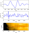 |
Fig. 11. Top: evolution of the vT component (blue) at the apex of loop F2 showing a damped oscillation following an event possibly associated with an impulsive temperature increase. A large-scale trend was removed from the vT time-series by fitting and subtracting a second-degree polynomial. Middle: evolution of the vT component at the apex of loop F3 showing a sustained oscillation. Bottom: sustained oscillation in the time–distance plot of forward-modelled SDO/AIA 171 Å emission. |
For the oscillatory motions seen in the simulation in magnetic structures, both ‘decaying’ and ‘decayless’ regimes correspond to standing transverse oscillations, with the oscillation antinodes lying at coronal heights, and are therefore consistent with the observations of transverse oscillations of coronal loops as seen in TRACE and SDO/AIA data (e.g., Aschwanden et al. 1999; White & Verwichte 2012), where the standing transverse oscillation is the most commonly observed regime.
We further note that the detected oscillation periods vary between different field lines and can also change with time, particularly in loops that are subject to change in physical properties, or with increasing or decreasing loop length, as would be expected for standing oscillations (this is true for all oscillation modes visible in the simulation). This spread and variability of the oscillation periods and lack of oscillation coherence in different parts of the simulation domain suggest that the oscillations are not a result of a coherent global oscillation in the simulation. Our analysis therefore does not agree with the premise that the transverse oscillations in the corona are driven by the global p-mode oscillation which is based on the comparison of peaks in the power spectra from velocity measurements in the corona and the p-mode power spectra (Morton et al. 2016, 2019); it should nevertheless be noted that analysis in such studies focuses on very long coronal loops, that is, the spatial scales are very different from the short low-lying loops studied in this work. Such a mechanism requires coronal loops to oscillate with the same period regardless of their length, as they are driven at their footpoints by a harmonic driver. The variability of the oscillation period in the simulation therefore excludes the presence of a harmonic driver, or at the very least suggests that such a driver is not the dominant mechanism responsible for the excitation of transverse oscillations in this work. We stress that care should be taken when drawing conclusions from the global power spectra in light of the temporal variability of the oscillation periods of individual magnetic structures which has been shown both observationally (Verwichte & Kohutova 2017) and by numerical simulations (Kohutova & Verwichte 2017).
The excitation mechanism proposed by Nakariakov et al. (2016) is based on identifying the decayless oscillations as self-oscillations of the coronal loop that are excited by interaction with quasi-steady flows similar to a bow moving across a violin string. The flows in the simulation domain are too dynamic and not stable enough to drive persistent self-oscillation of the field lines; this is evidenced by the motion of loop footpoints that are dragged around by turbulent flows in the lower solar atmosphere shown in Fig. 10 and show variability on the order of minutes. However, 3D numerical models seem to suggest that excitation of self-oscillations requires persistent flows that are steady on timescales of the order of an hour (Karampelas & Van Doorsselaere 2020).
The absence of increased oscillatory power in the chromosphere at the positions of the footpoints of the oscillating field lines also suggests that a harmonic footpoint driver is not a prerequisite for the excitation of coronal oscillations. Open questions as to the excitation mechanism of the decayless oscillations therefore still remain. If this latter mechanism is global, it is unclear as to why they are they not observed in all coronal loops. The decayless oscillations are sufficiently abundant to rule out an isolated event (Anfinogentov et al. 2015), but are insufficiently abundant to suggest that they are driven by a global process.
Finally, the differences between the magnetic and density structure of the simulated and real solar corona, and hence the limitations of the model used for our analysis need to be addressed. The forward-modelled EUV emission from the simulated corona is comparatively more diffuse and lacks a lot of fine-scale structure seen in real coronal observations, especially fine-scale coronal strands revealed by observations from the second Hi-C flight (Williams et al. 2020), which are not resolved in SDO/AIA observations. The simulated corona also suffers from a lack of coronal loops, which are understood in the traditional sense as distinct structures denser than the surroundings with distinct boundaries. As the simulation does not include any flux emergence, the coronal loops in the simulation do not correspond to overdense flux tubes lifted into the corona from the lower solar atmosphere but are instead filled with evaporated plasma due to impulsive heating events. Because enhanced heating regions have an irregular shape (Kohutova et al. 2020a), the structures filled with evaporated plasma have a greater spatial extent and lack well-defined boundaries. Simulation resolution might also be a limiting factor, although the characteristic transverse scales seen in time–distance plots are well above the horizontal grid size of 48 km. However, distinct oscillating strands are however still observable in Fig. 2. Furthermore, recent numerical studies of the evolution of initially homogeneous coronal loops as a response to transverse motions suggest that our highly idealised picture of coronal loops as monolithic plasma cylinders is unlikely to be realistic in the first place (Magyar & Van Doorsselaere 2018; Karampelas et al. 2019; Antolin & Van Doorsselaere 2019).
6. Conclusions
We studied the excitation and evolution of coronal oscillations in 3D self-consistent simulations of solar atmosphere spanning from the convection zone to the solar corona using the radiation-MHD code Bifrost. We combined forward-modelled EUV emission with 3D tracing of magnetic field through both space and time in order to analyse the oscillatory behaviour of individual magnetic loops, while accounting for their dynamic evolution. We analysed the evolution of different velocity components using wavelet analysis to capture changes in the oscillatory periods caused by evolution of the properties of the oscillating magnetic loops. Various types of oscillations commonly observed in the corona are reproduced in the simulations. We detect standing oscillations in both transverse and longitudinal velocity components, including higher order oscillation harmonics. We further show that self-consistent simulations reproduce two distinct regimes of transverse coronal oscillations, that is rapidly decaying oscillations triggered by impulsive events and sustained small-scale oscillations showing no observable damping. Damped transverse oscillations are found to be associated with instances of impulsive energy release, such as small-scale reconnection events or external perturbations leading to sudden changes in the loop properties, in agreement with coronal observations. Persistent transverse oscillations on the other hand are not linked to any such impulsive events. We do not find any evidence for this oscillation regime being driven by a global (simulation) p-mode. Lack of enhanced oscillatory power near the footpoint regions of the studied loops together with variability of oscillation periods between different coronal loops and lack of oscillation coherence across the simulation domain exclude any type of harmonic driver as being responsible for the excitation of the oscillations.
Our work therefore highlights the complexity of coronal oscillations in simulations with realistic magnetic field configurations which include the complex dynamics of the lower solar atmosphere. Care needs to be taken when translating findings from highly idealised models into real solar observations, as there are several limitations to treating coronal loops as static structures. Here, we show that individual field lines are very dynamic, their footpoints migrate, and their overall length changes significantly over realistic timescales. This might have non-negligible consequences for the accuracy of estimates of coronal plasma parameters deduced using coronal seismology. The oscillating coronal structures we analysed are far from idealised plasma cylinders. The focus of modelling work should therefore be shifting from rigid cylindrical models towards more realistic descriptions that account for rapid variability, complex morphology, and the presence of non-linearities. There are obviously natural limitations to this approach resulting from the computational expense of building such models and also from the associated limits on the physical size of the simulation domain. Work is currently underway to investigate the evolution of coronal loops in 3D self-consistent simulations that span high into the corona. We would therefore like to highlight the potential of using self-consistent simulations of the solar atmosphere as a laboratory for testing assumptions made by coronal seismology and models of various damping and dissipation mechanisms in an environment with realistic density structure and magnetic field geometry.
Movies
Movie of Fig. 2 Access here
Movie of Fig. 4 Access here
Movie of Fig. 10 Access here
Acknowledgments
This research was supported by the Research Council of Norway through its Centres of Excellence scheme, project no. 262622 and through grants of computing time from the Programme for Supercomputing.
References
- Afanasyev, A. N., Van Doorsselaere, T., & Nakariakov, V. M. 2020, A&A, 633, L8 [NASA ADS] [CrossRef] [EDP Sciences] [Google Scholar]
- Anfinogentov, S. A., Nakariakov, V. M., & Nisticò, G. 2015, A&A, 583, A136 [NASA ADS] [CrossRef] [EDP Sciences] [Google Scholar]
- Antolin, P., & Van Doorsselaere, T. 2019, Front. Phys., 7, 85 [Google Scholar]
- Antolin, P., Yokoyama, T., & Van Doorsselaere, T. 2014, ApJ, 787, L22 [NASA ADS] [CrossRef] [Google Scholar]
- Aschwanden, M. J., Fletcher, L., Schrijver, C. J., & Alexander, D. 1999, ApJ, 520, 880 [NASA ADS] [CrossRef] [Google Scholar]
- Berghmans, D., & Clette, F. 1999, Sol. Phys., 186, 207 [NASA ADS] [CrossRef] [Google Scholar]
- Carlsson, M., Hansteen, V. H., & Gudiksen, B. V. 2010, Mem. Soc. Astron. It., 81, 582 [Google Scholar]
- Carlsson, M., Hansteen, V. H., Gudiksen, B. V., Leenaarts, J., & De Pontieu, B. 2016, A&A, 585, A4 [NASA ADS] [CrossRef] [EDP Sciences] [Google Scholar]
- Chen, F., & Peter, H. 2015, A&A, 581, A137 [NASA ADS] [CrossRef] [EDP Sciences] [Google Scholar]
- De Moortel, I. 2005, Phil. Trans. R. Soc. A, 363, 2743 [Google Scholar]
- De Moortel, I., & Nakariakov, V. M. 2012, Phil. Trans. R. Soc. A, 370, 3193 [NASA ADS] [CrossRef] [Google Scholar]
- De Moortel, I., & Pascoe, D. J. 2012, ApJ, 746, 31 [NASA ADS] [CrossRef] [Google Scholar]
- De Moortel, I., Ireland, J., & Walsh, R. W. 2000, A&A, 355, L23 [NASA ADS] [Google Scholar]
- De Pontieu, B., Erdélyi, R., & James, S. P. 2004, Nature, 430, 536 [NASA ADS] [CrossRef] [PubMed] [Google Scholar]
- Duckenfield, T., Anfinogentov, S. A., Pascoe, D. J., & Nakariakov, V. M. 2018, ApJ, 854, L5 [NASA ADS] [CrossRef] [Google Scholar]
- Edwin, P. M., & Roberts, B. 1983, Sol. Phys., 88, 179 [Google Scholar]
- Eklund, H., Wedemeyer, S., Snow, B., et al. 2021, Phil. Trans. R. Soc. A, 379, 20200185 [Google Scholar]
- Felipe, T. 2012, ApJ, 758, 96 [NASA ADS] [CrossRef] [Google Scholar]
- González-Morales, P. A., Khomenko, E., & Cally, P. S. 2019, ApJ, 870, 94 [CrossRef] [Google Scholar]
- Goossens, M. L., Arregui, I., & Van Doorsselaere, T. 2019, Front. Astron. Space Sci., 6, 20 [Google Scholar]
- Gudiksen, B. V., Carlsson, M., Hansteen, V. H., et al. 2011, A&A, 531, A154 [NASA ADS] [CrossRef] [EDP Sciences] [Google Scholar]
- Karampelas, K., & Van Doorsselaere, T. 2020, ApJ, 897, L35 [Google Scholar]
- Karampelas, K., Van Doorsselaere, T., & Antolin, P. 2017, A&A, 604, A130 [NASA ADS] [CrossRef] [EDP Sciences] [Google Scholar]
- Karampelas, K., Van Doorsselaere, T., & Guo, M. 2019, A&A, 623, A53 [NASA ADS] [CrossRef] [EDP Sciences] [Google Scholar]
- Kohutova, P., & Verwichte, E. 2017, A&A, 606, A120 [NASA ADS] [CrossRef] [EDP Sciences] [Google Scholar]
- Kohutova, P., & Verwichte, E. 2018, A&A, 613, L3 [NASA ADS] [CrossRef] [EDP Sciences] [Google Scholar]
- Kohutova, P., Antolin, P., Popovas, A., Szydlarski, M., & Hansteen, V. H. 2020a, A&A, 639, A20 [EDP Sciences] [Google Scholar]
- Kohutova, P., Verwichte, E., & Froment, C. 2020b, A&A, 633, L6 [NASA ADS] [CrossRef] [EDP Sciences] [Google Scholar]
- Leenaarts, J., Carlsson, M., & Rouppe van der Voort, L. 2015, ApJ, 802, 136 [Google Scholar]
- Liu, J., Nelson, C. J., Snow, B., Wang, Y., & Erdélyi, R. 2019, Nat. Commun., 10, 3504 [NASA ADS] [CrossRef] [Google Scholar]
- Magyar, N., & Van Doorsselaere, T. 2016, A&A, 595, A81 [NASA ADS] [CrossRef] [EDP Sciences] [Google Scholar]
- Magyar, N., & Van Doorsselaere, T. 2018, ApJ, 856, 144 [Google Scholar]
- Magyar, N., Van Doorsselaere, T., & Marcu, A. 2015, A&A, 582, A117 [NASA ADS] [CrossRef] [EDP Sciences] [Google Scholar]
- Morton, R. J., Tomczyk, S., & Pinto, R. F. 2016, ApJ, 828, 89 [NASA ADS] [CrossRef] [Google Scholar]
- Morton, R. J., Weberg, M. J., & McLaughlin, J. A. 2019, Nat. Astron., 3, 223 [NASA ADS] [CrossRef] [Google Scholar]
- Nakariakov, V. M., & Kolotkov, D. Y. 2020, ARA&A, 58, 441 [Google Scholar]
- Nakariakov, V. M., & Verwichte, E. 2005, Liv. Rev. Sol. Phys., 2, 3 [Google Scholar]
- Nakariakov, V. M., Ofman, L., Deluca, E. E., Roberts, B., & Davila, J. M. 1999, Science, 285, 862 [Google Scholar]
- Nakariakov, V. M., Tsiklauri, D., Kelly, A., Arber, T. D., & Aschwanden, M. J. 2004, A&A, 414, L25 [NASA ADS] [CrossRef] [EDP Sciences] [Google Scholar]
- Nakariakov, V. M., Anfinogentov, S. A., Nisticò, G., & Lee, D.-H. 2016, A&A, 591, L5 [NASA ADS] [CrossRef] [EDP Sciences] [Google Scholar]
- Nisticò, G., Nakariakov, V. M., & Verwichte, E. 2013, A&A, 552, A57 [NASA ADS] [CrossRef] [EDP Sciences] [Google Scholar]
- Pagano, P., & De Moortel, I. 2017, A&A, 601, A107 [NASA ADS] [CrossRef] [EDP Sciences] [Google Scholar]
- Pagano, P., & De Moortel, I. 2019, A&A, 623, A37 [NASA ADS] [CrossRef] [EDP Sciences] [Google Scholar]
- Peter, H., Bingert, S., Klimchuk, J. A., et al. 2013, A&A, 556, A104 [NASA ADS] [CrossRef] [EDP Sciences] [Google Scholar]
- Riedl, J. M., Van Doorsselaere, T., & Santamaria, I. C. 2019, A&A, 625, A144 [CrossRef] [EDP Sciences] [Google Scholar]
- Santamaria, I. C., Khomenko, E., & Collados, M. 2015, A&A, 577, A70 [NASA ADS] [CrossRef] [EDP Sciences] [Google Scholar]
- Shelyag, S., Keys, P., Mathioudakis, M., & Keenan, F. P. 2011, A&A, 526, A5 [NASA ADS] [CrossRef] [EDP Sciences] [Google Scholar]
- Stein, R. F., & Nordlund, Å. 2001, ApJ, 546, 585 [NASA ADS] [CrossRef] [Google Scholar]
- Tomczyk, S., & McIntosh, S. W. 2009, ApJ, 697, 1384 [NASA ADS] [CrossRef] [Google Scholar]
- Torrence, C., & Compo, G. P. 1998, Bull. Am. Meteorol. Soc., 79, 61 [Google Scholar]
- Van Doorsselaere, T., Antolin, P., Yuan, D., Reznikova, V., & Magyar, N. 2016, Front. Astron. Space Sci., 3, 4 [NASA ADS] [CrossRef] [Google Scholar]
- Verwichte, E., & Kohutova, P. 2017, A&A, 601, L2 [NASA ADS] [CrossRef] [EDP Sciences] [Google Scholar]
- Verwichte, E., Nakariakov, V. M., Ofman, L., & Deluca, E. E. 2004, Sol. Phys., 223, 77 [NASA ADS] [CrossRef] [Google Scholar]
- Verwichte, E., Van Doorsselaere, T., Foullon, C., & White, R. S. 2013, ApJ, 767, 16 [NASA ADS] [CrossRef] [Google Scholar]
- Wang, T., Ofman, L., Davila, J. M., & Su, Y. 2012, ApJ, 751, L27 [Google Scholar]
- White, R. S., & Verwichte, E. 2012, A&A, 537, A49 [NASA ADS] [CrossRef] [EDP Sciences] [Google Scholar]
- Williams, T., Walsh, R. W., Winebarger, A. R., et al. 2020, ApJ, 892, 134 [Google Scholar]
All Tables
All Figures
|
Fig. 1. Left: magnetic configuration of the simulation showing the temperature profile of the individual field lines. The simulation domain has physical size of 24 × 24 × 16.8 Mm. The simulation snapshot shown corresponds to t = 180 s after the non-equilibrium ionisation of hydrogen has been switched on. Right: line-of-sight component Bz of the photospheric magnetic field at t = 180 s. |
| In the text | |
|
Fig. 2. Left: forward-modelled emission in the SDO/AIA 171 Å channel at t = 180 s. Dashed lines outline projected positions of the studied field lines F1−F5. Right: time–distance plots showing temporal evolution along the slits shown in blue. The vertical axis corresponds to the distance along the slit. Several oscillating structures are visible in the time–distance plots. The dashed contour in plot A outlines a propagating disturbance. An animation of this figure is available online. |
| In the text | |
|
Fig. 3. Forward-modelled emission in the SDO/AIA 171 Å channel at t = 180 s viewed along the y-axis. Dashed lines outline the projected positions of the studied field lines F1−F5. |
| In the text | |
|
Fig. 4. Left: location of field lines F1−F5 chosen for analysis of oscillatory behaviour shown at t = 1500 s. We also show the z-component of vorticity ωz at z = 0, i.e. in the photosphere. The footpoints of analysed field lines are embedded in the intergranular lanes with strong vortex flows. Right: configuration viewed from above. An animation of this figure is available online. |
| In the text | |
|
Fig. 5. Left: evolution of temperature, density and three velocity components vL, vT and vV along the field line F1. The x axis corresponds to time and the y axis corresponds to the position along the field line. Vertical dotted lines mark segments with oscillatory behaviour. Top right: evolution of the transverse component of the velocity vT at the footpoints FP1 and FP2 (red and blue respectively) 1 Mm above the transition region and at the fieldline apex halfway between the two footpoints (green). Bottom right: wavelet spectra for the three velocity components taken at the apex of the field line and at the footpoints FP1 and FP2. Dark colour corresponds to high power. The hatched region corresponds to the area outside of the cone of influence. White lines correspond to 95% significance contours. |
| In the text | |
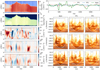 |
Fig. 6. Same as Fig. 5, but for field line F2. |
| In the text | |
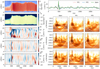 |
Fig. 7. Same as Fig. 5, but for field line F3. |
| In the text | |
 |
Fig. 8. Same as Fig. 5, but for field line F4. |
| In the text | |
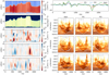 |
Fig. 9. Same as Fig. 5, but for field line F5. |
| In the text | |
|
Fig. 10. Top: integrated power between 1.67 mHz and 16.7 mHz for vx (left), vy (centre) components of the velocity at z = 1.4 Mm in the chromophere and line-of-sight photospheric magnetic field at t = 180 s (right). Bottom: integrated power between 1.67 mHz and 16.7 mHz for vx (left), vy (centre) and vz (right) components of the velocity at z = 10 Mm in the corona. Coloured circles with 1 Mm diameter are centred on positions of footpoint coordinates at z = 1.4 Mm at t = 0 s and colour-coded as follows: F1-black, F2-red, F3-purple, F4-green, and F5-orange. An animation of this figure for the full duration of the simulation is available online. |
| In the text | |
|
Fig. 11. Top: evolution of the vT component (blue) at the apex of loop F2 showing a damped oscillation following an event possibly associated with an impulsive temperature increase. A large-scale trend was removed from the vT time-series by fitting and subtracting a second-degree polynomial. Middle: evolution of the vT component at the apex of loop F3 showing a sustained oscillation. Bottom: sustained oscillation in the time–distance plot of forward-modelled SDO/AIA 171 Å emission. |
| In the text | |
Current usage metrics show cumulative count of Article Views (full-text article views including HTML views, PDF and ePub downloads, according to the available data) and Abstracts Views on Vision4Press platform.
Data correspond to usage on the plateform after 2015. The current usage metrics is available 48-96 hours after online publication and is updated daily on week days.
Initial download of the metrics may take a while.